Hall equilibrium of thin Keplerian disks embedded in mixed poloidal and toroidal magnetic fields

Abstract

Axisymmetric steady-state weakly ionized Hall-MHD Keplerian thin disks are investigated by using asymptotic expansions in the small disk aspect ratio $\epsilon$. The model incorporates the azimuthal and poloidal components of the magnetic fields in the leading order in $\epsilon$. The disk structure is described by an appropriate Grad-Shafranov equation for the poloidal flux function $\psi$ that involves two arbitrary functions of $\psi$ for the toroidal and poloidal currents. The flux function is symmetric about the midplane and satisfies certain boundary conditions at the near-horizontal disk edges. The boundary conditions model the combined effect of the primordial as well as the dipole-like magnetic fields. An analytical solution for the Hall equilibrium is achieved by further expanding the relevant equations in an additional small parameter $\delta$ that is inversely proportional to the Hall parameter. It is thus found that the Hall equilibrium disks fall into two types: Keplerian disks with (i) small ($R_{d}\sim\delta^{0}$) and (ii) large (${R_{d}}\gtrsim\delta^{-k}$, $k>0$) radius of the disk. The numerical examples that are presented demonstrate the richness and great variety of magnetic and density configurations that may be achieved under the Hall-MHD equilibrium.

1 Introduction

In the present study the Hall equilibrium of thin Keplerian disks embedded in 3D axially-symmetric magnetic fields is investigated. Protoplanetary disks have been the subject of numerous investigations in search of possible instabilities that may play a significant role in such yet not totally understood phenomena as the outwards transfer of angular momentum, and planet formation. However, in most astrophysics-related hydromagnetic stability studies which include accretion, jet, and wind effects the models for the underlying equilibrium states are based on the local approximation or a ’cylindrical disk’ that is uniform in the axial direction. A more realistic model of thin disks is adopted in Regev (1983), Kluzniak & Kita (2000), Umurhan et al. (2006) for equilibrium nonmagnetized rotating disks (see also Ogilvie (1997) for Keplerian disks of ideal MHD plasmas) and is based on an asymptotic approach in the small aspect ratio of the disk. Traditionally, a big variety of geometrical configurations of axially symmetric steady-state equilibria are described through a few arbitrary functions of the poloidal magnetic flux. The latter satisfies the Grad-Shafranov (GS) type equations within both one-fluid and multifluid models of the plasmas (e.g. McClements & Thyagaraja (2001); Thyagaraja & McClements (2006), see also the earlier study by Lovelace et al. (1986), where in particular thin rotating disks have been discussed and references therein). Such solutions provide a base for their stability studies.

Although the magnetic field configuration in real disks is largely unknown and, as observations and numerical simulations indicate, toroidal magnetic component may be of the same order of magnitude, or some times dominate the poloidal field due to the differential rotation of the disk (see e.g. Terquem & Papaloizou (1996); Papaloizou & Terquem (1997); Hawley & Krolik (2002); Proga (2003)). As shown in the present study there are three kinds of possible equilibrium in thin rotating disks which can not be reduced from one to the other: (i) pure poloidal, (ii) pure toroidal and (iii) mixed toroidal and poloidal magnetic field equilibria. The first case has been considered within the ideal MHD model by Lovelace et al. (1986), and Ogilvie (1997). The second case, i.e. the pure toroidal magnetic field has been investigated within the Hall MHD model by Shtemler et al. (2007). The present study is aimed to describe numerous axially-symmetric equilibria in 3D axially-symmetric magnetic fields that contain both toroidal and poloidal components, i.e. case (iii) within the Hall MHD model in thin disk approximation.

While most of recent research has focused on the magnetohydrodynamic (MHD) description of magneto-rotational instability (MRI), the importance of the Hall electric field to such astrophysical objects as protoplanetary disks has been pointed out by Wardle (1999). Since then, such works as Balbus & Terquem (2001), Salmeron & Wardle (2003), Salmeron & Wardle (2005), Desch (2004), Urpin & Rudiger (2005), Rudiger & Kitchatinov (2005), and Pandey & Wardle (2008) have shed light on the role of the Hall effect in the modification of the MRIs. However, in addition to modifying the MRIs, the Hall electromotive force gives rise to a new family of instabilities in a density-stratified environment. That new family of instabilities is characterized by the Hall parameter $\pi_{H}$ of the order of unity ( $\pi_{H}$ is the ratio of the Hall drift velocity $V_{HD}$ to the characteristic velocity, where $V_{HD}=l_{i}^{2}\Omega_{i}/H_{*}$, $l_{i}$ and $\Omega_{i}$ are the inertial length and Larmor frequency of the ions, respectively, and $H_{*}$ is the density inhomogeneity length (see Huba (1991)). As shown by Liverts & Mond (2004), and Kolberg et al. (2005), the Hall electric field combined with radial density stratification gives rise to two modes of wave propagation. The first one is the stable fast magnetic penetration mode, while the second is a slow quasi-electrostatic mode that may become unstable for a short-enough density inhomogeneity length $H_{*}$. The latter is termed the Hall instability. Density stratifications also play a crucial role in the recently discussed starto-rotational instability. That instability is excited by the combined effect of vertical and radial density stratification.

The aim of the present work is, therefore to describe the various Hall equilibrium configurations of magnetic field and density in thin magnetized Keplerian disks as a first step towards a further study of their various density stratification-dependent instabilities. The following simplifying assumptions are adopted throughout the present work: the plasma is treated in a 3D axially symmetric magnetic field within the Hall MHD model. The problem inside the disk is treated within the thin-disk approximation, while the effects of the outer region is modeled by the boundary condition for the poloidal magnetic flux. Influence of the accretion, jet and wind effects are neglected in the thin-disk approximation (Ogilvie (1997)). A near Keplerian region of the rotating disk is considered that starts at some radial distance away from a central body. The influence of the latter on the Keplerian portion of the disk is modeled by a dipole-like contribution (singular at the disk axis) to the boundary condition for the poloidal magnetic flux at the near-horizontal disk edges. In addition, axial electrical currents that are localized in the central non-Keplerian regions of the disk are taken into account through the resulting toroidal magnetic field components within the rotating disk. Influence of the interstellar (primordial) magnetic field is modeled by specifying the contribution of the latter on the near-horizontal disk edges.

The paper is organized as follows. The dimensional governing equations, the normalization procedure, and the resulting non-dimensional system are presented in the next Section. Section 3 contains an asymptotic analysis of the Hall-equilibrium in the small aspect ratio as well as the derivation the appropriate GS equation for the flux function and the corresponding boundary conditions at the disk edge. In section 4 an analytic model is developed for the Hall equilibrium with the aid of asymptotic expansions in a newly defined small parameter inversely proportional to the Hall parameter. Numerical examples for different regimes of the equilibrium are presented in section 5. Summary and discussion are in section 6.

2 The physical model for THIN Keplerian DISKs

A rotating thin disks is considered that is under the influence of a general 3D axially-symmetric magnetic field, as well as the gravitational field due to a massive central body. Electron inertia and pressure, displacement current, viscosity and radiation effects are neglected in the electrons momentum equation. Consequently the latter is reduced to the generalized Ohm law that takes into account the Hall effect. In addition the plasma is assumed to be quasi-neutral.

2.1 The basic equations

Under the assumptions mentioned above the physical model of the rotating magnetized disk is given by:

$$\frac{\partial n}{\partial t}+\nabla\cdot(n{\bf{V}})=0,\\$$ (1)

$$m_{i}n\frac{D\bf{V}}{Dt}=-\nabla P+\frac{1}{c}{\bf{j}}\times{\bf{B}}-m_{i}n\nabla\Phi,\\$$ (2)

$$\frac{D}{Dt}(Pn^{-\gamma})=0,\\$$ (3)

$$\frac{\partial{\bf{B}}}{\partial t}+c\nabla\times{\bf{E}}=0,\,\nabla\cdot{\bf{B}}=0,$$ (4)

$${\bf{E}}=-\frac{1}{c}{\bf{V}}\times{\bf{B}}+\frac{1}{ec}\frac{\bf{j}\times\bf{B}}{n_{e}},\,\,\,{\bf{j}}=\frac{c}{4{\pi}}\nabla\times{\bf{B}}.\,\,\,\,$$ (5)

Here the standard cylindrical coordinates $\{r,\theta,z\}$ are adopted throughout the paper with the associated unit basic vectors $\{\bf{i}_{r},\bf{i}_{\theta},\bf{i}_{z}\}$; $\bf{V}$ is the plasma velocity; $t$ is time; $D/Dt=\partial/\partial t+(\bf{V}\cdot\nabla)$ is the material derivative; $\Phi(R)=-GM_{c}/R$ is the gravitational potential of the central object; $R^{2}=r^{2}+z^{2}$; $G$ is the gravitational constant; $M_{c}$ is the total mass of the central object. The electric field $\bf{E}$ is described by the generalized Ohm’s law which is derived from the momentum equation for the electrons fluid by neglecting the electrons inertia and pressure; $\bf{B}$ is the magnetic field, $\bf{j}$ current density; $\gamma$ is the polytrophic coefficient, ($\gamma=5/3$ in the adiabatic case). $P=P_{e}+P_{i}+P_{n}$ is the total plasma pressure; $c$ is speed of light; $P_{l}$ and $m_{l}$ are the species pressures and masses ($l=e,i,n$ ), subscripts $e$, $i$ and $n$ denote the electrons, ions and neutrals, respectively; $e$ is the electron charge; $m_{i}=Zm_{p}$, $m_{p}$ is the proton mass ($Z=1$ for simplicity). Since the plasma is assumed to be quasi-neutral and partially ionized with small ionization degree and strongly coupled ions and neutrals

$$n_{e}\approx n_{i}\approx\alpha n_{n},n\approx n_{n},\alpha={n_{e}/(n_{e}+n_{n})}<<1,V_{i}\sim V_{n}.$$ (6)

In real protoplanetary disks, the electron density is determined by ionization versus recombination, and the fractional ionization may vary significantly in space. In such cases, rate equations that describe the ionization degree should be employed. However, in the present study the ionization fraction is assumed to be constant. This simplification is made to avoid the widely uncertain physics of ionization and recombination. Nevertheless, such approximation allows one to roughly estimate the real characteristics of the equilibrium system (see a discussion in section 5 in Shtemler et al. (2007)).

2.2 Scaling procedure

The physical variables are now transformed into nondimensional variables:

$$f_{nd}=f/f_{*},$$ (7)

where $f$ and $f_{nd}$ stand for any of the physical dimensional and non-dimensional variables, while the characteristic scales $f_{*}$ are defined as follows:

$$V_{*}=\Omega_{*}r_{*},\,\,t_{*}=\frac{1}{\Omega_{*}},\,\,\Phi_{*}={V_{*}}^{2},\,\,m_{*}=m_{i},\,\,n_{*}=n_{n},\,\,\,P_{*}=K(m_{*}n_{*})^{\gamma},\,\,\,\,j_{*}=\frac{c}{4\pi}\frac{B_{*}}{r_{*}},\,\,E_{*}=\frac{V_{*}B_{*}}{c}.$$ (8)

Here $\Omega_{*}=(GM_{c}/r_{*}^{3})^{1/2}$ is the Keplerian angular velocity of the fluid at the characteristic radius $r_{*}$ that belongs to the Keplerian portion of the disk; $K$ is the dimensional constant in the steady-state polytropic law $P=Kn^{\gamma}$. The characteristic values of the electric current and field, $j_{*}$ and $E_{*}$, have been chosen consistently with Maxwell equations. The characteristic dimensional magnetic field $B_{*}$ is specified below. Note that a preferred direction is tacitly defined here, namely, the positive direction of the $z$ axis is chosen according to positive Keplerian rotation.

The resulting dimensionless system (omitting the subscript ${}^{\prime}nd^{\prime}$ from the dimensionless variables) is given by:

$$\frac{\partial n}{\partial t}+\nabla\cdot(n{\bf{V}})=0,\,\,\,\,\,\,\,\,\,\,\,\,\,\,$$ (9)

$$n\frac{D\bf{V}}{Dt}=-\frac{1}{M_{S}^{2}}\nabla P+\frac{1}{\beta M_{S}^{2}}{\bf{j}}\times{\bf{B}}-n\nabla\Phi,\,\,\,\Phi(r,z)=-{1\over(r^{2}+z^{2})^{1/2}},$$ (10)

$$\frac{D(Pn^{-\gamma})}{Dt}=0,$$ (11)

$$\frac{\partial{\bf{B}}}{\partial t}+\nabla\times{\bf{E}}=0,\,\nabla\cdot{\bf{B}}=0,$$ (12)

$${\bf{E}}=-{\bf{V}}\times{\bf{B}}+\Pi_{H}\frac{\bf{j}\times\bf{B}}{n},\,\,\,\,{\bf{j}}=\nabla\times{\bf{B}}.$$ (13)

Here $M_{S}$ and $\beta$ are the Mach number and plasma beta, and $\Pi_{H}$ is the Hall coefficient in the generalized Ohm’ law (13):

$$M_{S}=\frac{V_{*}}{c_{S*}},\,\,\,\beta=4\pi\frac{P_{*}}{B_{*}^{2}},\,\,\,\Pi_{H}=\frac{\Omega_{i}}{\Omega_{*}}\bigg{(}\frac{l_{i}}{r_{*}}\bigg{)}^{2}\equiv\frac{B_{*}c}{4\pi e\alpha n_{*}\Omega_{*}r^{2}_{*}},$$ (14)

$c_{S*}=\sqrt{P_{*}/(m_{*}n_{*})}$ is the characteristic sound velocity, $l_{i}=c/\omega_{pi}$ and $\Omega_{i}=eB_{*}/(m_{*}c)$ are the inertial length and the Larmor frequency of ions, respectively, $\omega_{pi}=\sqrt{4\pi e^{2}\alpha n_{*}/m_{*}}$ is the plasma frequency of the ions. The increasing importance of the Hall term for weakly ionized disks is apparent as $\Pi_{H}$ is inversely proportional to the ionization degree $\alpha$.

A common property of thin Keplerian disks is their highly compressible motion with large Mach numbers $M_{S}$. Furthermore, the characteristic effective semi-thickness $H_{*}=H(r_{*})$ of the disk ($H=H(r)$ is the local disk height) is such that the disk aspect ratio $\epsilon$ equals the inverse Mach number:

$$\frac{1}{M_{S}}=\epsilon=\frac{H_{*}}{r_{*}}\lesssim 1.$$ (15)

The smallness of $\epsilon$ means that dimensional axial coordinate $|z|\leq H$ is also small, i.e. $z/r_{*}\sim\epsilon$, and the following rescaled values of the order of unity in $\epsilon$ may be introduced in order to further apply the asymptotic expansions in $\epsilon$ (Shtemler et al 2007):

$$\zeta=\frac{z}{\epsilon},\,\,\,h=\frac{H}{\epsilon},\,\,\,\pi_{H}=\frac{\Pi_{H}}{\epsilon},$$ (16)

where as was mentioned in the introduction, the rescaled Hall parameter $\pi_{H}$ is determined in terms of the characteristic disk thickness $H_{*}=\epsilon r_{*}$ as the density inhomogeneity length.

2.3 Physical conditions in protoplanetary disks

Before turning to the detailed description of the Hall equilibrium of rotating Keplerian disks it is instructive to estimate some of the parameters that have been introduced in the previous subsection. Typical protoplanetary disks extend up to the order of $100AU$ and consist of molecular gas with characteristic ion masses between $30m_{p}$ to $40m_{p}$. The temperature within a radius of about $0.1AU$ may exceed $10^{3}K$ were as further away from the central star the temperature decreases and may reach values of about $10K$ in the outer regions of the disk. As a result, while in the inner regions of the disk thermal collisions provide the dominant ionization mechanism, in regions beyond about $0.1AU$ the only sources of ionization are nonthermal, like cosmic rays and the decay of radioactive elements (Umebayashi & Nakano (1988), Gammie (1996), Igea & Glassgold (1999)). Taking that into account, the frequently used model is employed, in which the radial temperature profile is given by

$$T(r)=280\large(\frac{r}{1AU}\large)^{-1/2}\;\;\;\;K,$$ (17)

while the column mass density is given by the minimum mass model as

$$\Sigma(r)=1700\large(\frac{r}{1AU}\large)^{-3/2}\;\;\;\;g\;cm^{-2}.$$ (18)

The thickness of the disk as well as the neutral number density radial profiles may be calculated from the two functions above. The ionization fraction is given by

$$\alpha=\sqrt{\frac{\xi}{n\beta_{r}}},$$ (19)

where $\xi$, the ionization rate due to the non thermal processes, is given by

$$\xi=10^{-17}exp(-\Sigma/192)+7\times 10^{-23}\;\;\;\;sec^{-1},$$ (20)

and $\beta_{r}$ is the dissociative recombination rate given by

$$\beta_{r}=1.1\times 10^{-7}\large(\frac{T}{300K}\large)^{-1}\;\;\;\;cm^{3}\;sec^{-1}.$$ (21)

A detailed and critical study of the model as well as some other suggestions may be found in Hayashi et al. (1985), Gammie (1996), Fromang et al. (2002), Sano & Stone (2002). Here however, Eqs. (17)-(21) are employed in order to obtain a rough estimate for the physical conditions in the disk. To do that, attention is focused on two representative radii, $r_{1}=1AU$ and $r_{2}=20AU$. A characteristic magnetic field of $0.1G$ is assumed while the mass of the central star has been assumed to be one solar mass. The results are summarized in Table (1). The increase in the rescaled Hall parameter is due to the decrease in the neutrals number density that compensates for the increase in the ionization fraction and the angular momentum per unit mass. In particular, it is evident that the entire disk resides within the Hall regime.

Table 1: Estimation of the physical conditions at two radii within the disk

$~{}~{}r_{*}\;AU~{}~{}$	$~{}~{}~{}~{}\alpha~{}~{}$	$~{}~{}~{}l_{i}\;Km~{}~{}$	$~{}~{}~{}\pi_{H}~{}~{}$	$~{}~{}~{}\omega_{pi}\;sec^{-1}~{}~{}$	$~{}~{}~{}\Omega_{*}\;sec^{-1}~{}~{}$
1	$1.12\times 10^{-14}$	$1.24\times 10^{3}$	1.03	241.6	$2.00\times 10^{-7}$
20	$4.14\times 10^{-13}$	$1.25\times 10^{4}$	11.2	23.82	$2.23\times 10^{-9}$

3 HALL EQUILIBRIUM IN THIN DISKS IN 3D AXISYMMETRICAL MAGNETIC FIELDS

In magnetized disks the solution of the steady-state equilibrium problem ($\partial/\partial t\equiv 0$) may be obtained within the Keplerian portion of a disk by asymptotic expansions in small $\epsilon$ with the aid of Eqs. (9)-(16) (similar to Regev (1983), Ogilvie (1997), Kluzniak & Kita (2000), Umurhan et al. (2006), and Shtemler et al. (2007)). This yields for the gravitational potential in the Keplerian portion of the disk:

$$\Phi(r,\zeta)=-\frac{1}{r}+\frac{\epsilon^{2}\zeta^{2}}{2r^{3}}+O(\frac{\epsilon^{4}}{r^{5}}),\,\,\,\epsilon\ll r,\,\,\zeta\sim\epsilon^{0}.$$ (22)

To leading order in $\epsilon$ within the thin disk approximation, the toroidal velocity $V_{\theta}$ is described by the Keplerian law, which follows from the leading order radial component of the momentum equation:

$${\bf{V}}=V_{\theta}{\bf{i}}_{\theta},\,\,\,V_{\theta}=\Omega(r)r,\,\,\,\Omega(r)=r^{-3/2},\,\,\,V_{\theta}\sim\epsilon^{0},\,\,\,V_{r}\sim\epsilon,\,\,\,V_{z}\sim\epsilon^{2}.$$ (23)

The asymptotic orders in $\epsilon$ in equilibrium relations (23) are similar to those in Ogilvie (1997). They may be inferred by observing that due to Eq. (9) ($\nabla\cdot(n{\bf{V}})=0$) the axisymmetric fluid momentum per unit volume is expressed in terms of a scalar stream function $\chi(r,\zeta)$

$$n{\bf{V}}=nV_{\theta}{\bf{i}}_{\theta}+\frac{1}{r}\hat{\nabla}\chi\times{\bf{i}}_{\theta},\,\,\,\big{(}\hat{\nabla}={\bf{i}}_{r}\frac{\partial}{\partial r}+{\bf{i}}_{z}\frac{1}{\epsilon}\frac{\partial}{\partial\zeta}\big{)}.$$ (24)

Assuming now that the toroidal velocity component is dominant, and noticing that $\partial/\partial z\sim\epsilon^{-1}$ imply that $\chi\sim\epsilon^{2}$, which immediately results in the ordering presented in Eq. (23) (see also discussion just after Eq. (41) ).

By a similar way the divergent free axisymmetric magnetic field $\bf{B}$, ($\nabla\cdot\bf{B}=0$) is written in terms of a poloidal flux function $\Psi(r,\zeta)$ in the following way:

$${\bf{B}}=B_{\theta}{\bf{i}}_{\theta}+\frac{1}{r}\hat{\nabla}\Psi\times{\bf{i}}_{\theta},\,\,\,\Psi(r,\zeta)=\Psi_{0}(r)+\epsilon\psi(r,\zeta),\,\,\,B_{r}=-\frac{1}{r}\frac{\partial\psi}{\partial\zeta},\,\,\,B_{z}=\frac{1}{r}\frac{d\Psi_{0}}{dr}+\epsilon\frac{1}{r}\frac{\partial\psi}{\partial r}.$$ (25)

Here the poloidal flux function $\Psi$ is presented as sum of $\Psi_{0}(r)$ and $\epsilon\psi(r,\zeta)$, which are scaled in $\epsilon$ by such a way to produce $B_{z}\sim B_{r}\sim\epsilon^{0}$ to leading order in the thin disk approximation.

Proceeding further it is noticed that Eq. (12) means that the electric field is derived from a potential $\phi(r,\zeta)$

$${\bf{E}}=\epsilon\hat{\nabla}\phi.$$ (26)

Taking now the dot product of both sides of Eq. (13) with the magnetic field reveals that ${\bf{B}}\cdot\hat{\nabla}\phi=0$, and therefore $\phi$ is a function of the magnetic flux, i.e.

$$\phi=\phi(\Psi),$$ (27)

which immediately, due to axisymmetry means that the toroidal component of the electric field vanishes, i.e., $E_{\theta}=0$. In order to impose that condition, Ampere’s law is first employed in order to write the electric current density in the following way:

$${\bf{j}}=j_{\theta}{\bf{i}}_{\theta}+\frac{1}{r}\hat{\nabla}(rB_{\theta})\times{\bf{i}}_{\theta},\,\,\,j_{r}=-\frac{1}{\epsilon}\frac{\partial B_{\theta}}{\partial\zeta},\,\,\,j_{\theta}=-\frac{1}{r}\frac{d}{dr}\big{(}\frac{d\Psi_{0}}{dr}\big{)}-\frac{1}{\epsilon}\frac{1}{r}\frac{\partial^{2}\psi}{\partial\zeta^{2}}-\epsilon\frac{\partial}{\partial r}\big{(}\frac{1}{r}\frac{\partial\psi}{\partial r}\big{)},\,\,\,j_{z}=\frac{1}{r}\frac{\partial(rB_{\theta})}{\partial r}.$$ (28)

Returning now to Eq. (13), the toroidal component of the electric field is given by:

$$E_{\theta}={\bf{B}}\cdot\hat{\nabla}(rB_{\theta})=0.$$ (29)

The leading order in $\epsilon$ of the last equation yields

$$\frac{\partial B_{\theta}}{\partial\zeta}\frac{d\Psi_{0}}{dr}=0,$$ (30)

which is satisfied if either $\partial B_{\theta}/\partial\zeta=0$ or $d\Psi_{0}/dr=0$. The former case was considered by Ogilvie (1997) within the classical MHD model for the equilibrium of a differentially rotating thin disk containing a pure poloidal magnetic field ($B_{\theta}\equiv 0$). The second case, for the pure toroidal magnetic field ($\Psi\equiv 0$) has been investigated within the Hall MHD model by Shtemler et al. (2007). Thus in the leading order in $\epsilon$, there are three possible equilibrium states: (i) pure toroidal, (ii) pure poloidal and (iii) mixed magnetic field equilibrium, which can not be reduced from one to the other. In the present work the case $\Psi_{0}\equiv 0$ is investigated within the Hall MHD model allowing for both toroidal as well as poloidal components of the magnetic field in the leading order. This results in:

$${\bf{B}}=B_{\theta}{\bf{i}}_{\theta}+\frac{1}{r}\hat{\nabla}\Psi\times{\bf{i}}_{\theta},\,\,\,\Psi(r,\zeta)=\epsilon\psi(r,\zeta),\,\,\,\phi=\phi(\psi),\,\,\,\,B_{r}=-\frac{1}{r}\frac{\partial\psi}{\partial\zeta},\,\,\,\hat{B}_{z}\equiv\frac{B_{z}}{\epsilon}=\frac{1}{r}\frac{\partial\psi}{\partial r},$$ (31)

where the magnetic flux function $\Psi$ is scaled with $\epsilon$ in such a way that the resulting radial component of the magnetic field is of the order of the toroidal one ($\sim\epsilon^{0}$) in the thin disk approximation, while the axial magnetic field $B_{z}$ is of order $\sim\epsilon$. Consequently Eqs. (29) and (31) yield

$$rB_{\theta}=I(\psi),$$ (32)

where according to Ampere’s law $I(\psi)$ is the current flowing through a circular area in the plane $\zeta=const$. Furthermore, now Ampere’s law may be written as follows:

$${\bf{E}}\equiv\epsilon\hat{\nabla}\phi=-{\bf{V}}\times{\bf{B}}+\epsilon\pi_{H}\frac{{\bf{j}}\times{\bf{B}}}{n}.$$ (33)

Finally note that the case of the pure toroidal magnetic field $\psi\equiv 0$ (i.e. ${\bf{B}}=(0,B_{\theta},0$)) requires a separate consideration. In that case the relation $E_{\theta}=0$ is satisfied identically, while Faraday’s law reduces to with the help to Eq. (33) to

$$\hat{\nabla}\times\big{[}\frac{rB_{\theta}}{N}\hat{\nabla}(rB_{\theta})\big{]}=0,$$ (34)

where $N=r^{2}n$ is the inertial moment density through the Keplerian disk. This leads to the familiar result up to the scaling factor $\pi_{H}$ (Shtemler et al. (2007)):

$$rB_{\theta}=I(N),\,\,\,\pi_{H}\phi=-\int_{0}^{N}\frac{I(N)\dot{I}(N)}{N}dN.$$ (35)

Here and everywhere below the upper dot denotes a derivative with respect to the argument.

Every thing is ready now to derive the relevant GS equation in the general case $\psi\neq 0$. The latter is indeed readily obtained by projecting Eq. (13) onto the $\hat{\nabla}\psi$ direction and taking into account the above relations. To leading order in $\epsilon$ the result is the following nonlinear differential equation for $\psi$, which depends parametrically on the radial coordinate $r$:

$$\frac{\partial^{2}\psi}{\partial\zeta^{2}}=-I(\psi)\dot{I}(\psi)-\frac{1}{\pi_{H}}N(r,\zeta)[\Omega(r)+\dot{\phi}(\psi)].$$ (36)

This is the GS equation (similar to Lovelace et al. (1986), McClements & Thyagaraja (2001) and references therein) that is modified for the special case of a thin disk in Hall MHD equilibrium. It interesting to note that in the limit of negligible Hall effect ($\pi_{H}\to 0$) Eq. (36) is reduced to the algebraic limit of the familiar isorotation law of ideal MHD that expresses the fluid’s angular momentum constancy on magnetic surfaces.

In general, a coupled problem should be considered inside and outside the Keplerian disk such that the edge of the disk $\zeta=h(r)$ is determined self-consistently. However, to avoid the solution of the outer problem, the following assumption that is supported by the observation data for some protoplanetary disks (Calvet et al. (2002)) is adopted:

$$h(r)\equiv const=1.$$ (37)

Furthermore, the differential equation (36) must be complemented by an appropriate boundary conditions at the disk edge $\zeta=h(r)$, as well as by symmetry condition at the midplane (assuming $\hat{B}_{z}$, as well as $B_{\theta}$ being even functions of $\zeta$):

$$n=0,\psi=\Gamma(r)\,\,\,\,\mbox{at}\,\,\,\,\zeta=h(r),\,\,\,\,\frac{\partial\psi}{\partial\zeta}=0\,\,\,\,\mbox{at}\,\,\,\,\zeta=0,$$ (38)

where $\Gamma(r)$ is a specified function. Since there is no direct observational information on how magnetic fields are distributed on disk edges the following specific equilibrium configurations are conjectured which are idealized representations of Keplerian disks. The value of $\hat{B}_{z}$ at the horizontal disk edges is assumed to be a sum of a constant primordial (Ogilvie (1997)) and a dipole-like (Lepeltier & Aly (1996), see also Lovelace et al. (2002), and Matt et al. (2002)) magnetic fields. The latter qualitatively reflects the effect of the central body on Keplerian portion of the disk. Below the two following configurations are examined:

$$\Gamma(r)=0.5Br^{2}-Mr^{-1},\,\,\,\,(B=\pm 1),$$ (39)

$$\Gamma(r)=-Mr^{-1},\,\,\,\,(B=0,\,\,M=\pm 1),$$ (40)

where the constants $B$ and $M$ are the dimensionless primordial magnetic field strength, and the moment of the dipole-like magnetic field, respectively. In the case (39) the characteristic magnetic field $B_{*}$ is chosen to be equal to the primordial magnetic field, while in the case (40) of zero primordial magnetic field, $B_{*}$ is chosen to make the dimensionless magnetic moment equal to unity. The signs of $B$ and $M$ depend on their directions with respect to positive direction determined by Keplerian rotation. Both $B$ and $M$ correspond to the magnetic flux function scaled by $\epsilon$, so the corresponding unscaled values are small constant of the order of $\epsilon$. Since the primordial magnetic field is likely much smaller than that of the dipole like magnetic field, the mixed case (39) with $B\sim M$ is rather a qualitative demonstration of the method ability to describe a wide variety of structures, while the case (40) assumes implicitly that the primordial magnetic field creates a much smaller input into the boundary conditions than the magnetic dipole. Although, in general the magnetic axis of the dipole is not aligned with the disk axis, some of the important problems, may be investigated analytically in an axisymmetric approach, which is valuable for subsequent full 3D analysis.

Note that Ohm’s law generalized for Hall equilibrium allows to integrate explicitly the vertical momentum balance equation in thin disk approximation. However, this procedure is singular in the limit of small Hall parameter. Employing Eqs. (33) and (23) in the axial component of the momentum equation (10) provides an explicit relation for the number density to the leading order in $\epsilon$:

$$n(r,\zeta)=\nu\big{[}\frac{2}{\beta\pi_{H}}\big{(}\phi(\psi)-\phi(\Gamma)\big{)}+\frac{2\Omega}{\beta\pi_{H}}\big{(}\psi-\Gamma\big{)}+\frac{1-\zeta^{2}}{r^{3}}\big{]}^{\frac{1}{\gamma-1}},\,\,\,\,\,N=r^{2}n,\,\,\,\,\,\nu=\big{(}\frac{\gamma-1}{2\gamma}\big{)}^{\frac{1}{\gamma-1}}.$$ (41)

Thus to the leading order, the momentum equation in the axial direction yields the density distribution (41), the momentum equation in the radial direction provides the Keplerian toroidal velocity $\sim\epsilon^{0}$, while the momentum equilibrium in the azimuthal direction along with the mass balance relation determine the radial and axial velocities to be small of the order of $\epsilon$ and $\epsilon^{2}$, respectively. Expression (41) is singular for vanishing $\pi_{H}$ and everywhere below the Hall parameter $\pi_{H}$, is assumed to be of the order of or much larger than unity.

Inspecting the resulting problem (36) and (41) reveals that it contains the Hall parameter $\pi_{H}$ in the two following combinations: as the ratio with inertial moment density $N/\pi_{H}$ in Eq. (36), and as a factor with the plasma beta $\beta\pi_{H}$ in Eq. (41). Since both plasma beta and Hall parameter are independent physical parameters, and since they are generally unknown in astrophysical systems, a scaled Hall plasma beta parameter is naturally introduced:

$$\beta_{H}=\beta\pi_{H}.$$ (42)

Note also that for large Hall plasma beta $\beta_{H}$, the arbitrary function $\phi(\psi)$ is dropped from Eqs. (41) and the number density is approaching its pure hydrodynamical limit.

The arbitrary functions $\phi(\psi)$ and $I(\psi)$ reflect the uncertainty of the steady-state equilibrium solution that as assumed here describes the equilibrium solution at long times. In general the corresponding initial value problem must be solved which shifts that uncertainty to the arbitrariness of the initial data (see e.g. Lovelace et al. 2002). The magnetic field and density structure is governed by the choice of the functions $\phi(\psi)$ and $I(\psi)$, here taken as following trial functions in order to qualitatively describe the equilibrium states:

$$I(\psi)=I^{(0)}+I^{(1)}\psi,\,\,\phi(\psi)=\phi^{(0)}+\phi^{(1)}\psi.$$ (43)

The constant $I^{(0)}$ is the total current through the disk that is localized along the axis (Shtemler et al. (2007)), while $\phi^{(0)}=0$ without loss of generality due to the physical meaning of the electric field potential (see also Eqs. (36) and (41)). Such kind simplest trial function are commonly used for ideal MHD model (see e.g. Wu & Chen (1989), Kaiser & Lortz (1995), Bogoyavlenskij (2000) and references therein for astrophysical applications). Sometimes the above relations are considered as first terms of generic expressions in which the arbitrary functions can be expanded in power series in $\psi$ (Bogoyavlenskij (2000)). Clearly, approximations (43) are biased by their partial form. However, in the present study it is conjectured that the main features of the equilibrium are rather general since relations (43) may be considered as a best fit linear approximations rather than first terms in appropriate Taylor’ sets.

To summarize, in the present model Hall MHD axisymmetric equilibria are determined up to the Hall parameter $\pi_{H}$, the Hall plasma beta parameter $\beta_{H}$, and the free constants $B$ and $M$ that characterize the primordial magnetic field and an effective magnetic dipole moment induced by the central body. In such equilibria the electric potential as well as the toroidal magnetic field are arbitrary functions of the magnetic flux, while the density is an explicit function of the coordinates and the magnetic flux function which satisfies a GS type equation modified for the special case of Hall equilibrium in thin-disk approximation.

4 ANALYSIS OF THE EQUILIBRIUM IN TERMS OF the scaled INVERSE HALL PARAMETER

Inspecting expression (41) for the inertial moment density $N$ and the GS equation (36) for the magnetic flux $\psi$ that contains $N/\pi_{H}$ reveals the existence of the following small parameter $\delta$:

$$\delta=\frac{\nu}{\pi_{H}}\lesssim 1.\,\,\,$$ (44)

In the adiabatic case with $\gamma=5/3$ adopted everywhere below, this parameter is indeed sufficiently small within the range from large values $\pi_{H}$ up to $\pi_{H}=1$ when it equals $\delta=\nu\approx 0.1$ (see definition of $\nu$ in Eq. (36)). Note also that validity for using $\delta=\nu/\pi_{H}$ as the small parameter is violated in the classical MHD limit ($\pi_{H}\to 0$) which requires a separate consideration.

Since the parameters of the equilibrium are widely arbitrary, two different families of equilibrium solutions are found, which correspond to either (i) small ( $\sim\delta$) or (ii) finite ( $\sim\delta^{0}$) deviations of the magnetic flux $\psi(r,\zeta)$ from its boundary value $\Gamma\sim\delta^{0}$. Note that the scaling in $\delta$ is applied to the flux function that is already scaled in $\epsilon$ (see Eqs. (25)), so that the dimensionless unscaled value $|\psi-\Gamma|$ is either (i) $\sim\epsilon\delta$ or (ii) $\sim\epsilon\delta^{0}$. Consequently, as will be seen below, the Hall equilibrium disks fall into two types which characterized by quite different orders in $\delta$: Keplerian disks with (i) small ($R_{d}\sim\delta^{0}$) and (ii) large (${R_{d}}\gtrsim\delta^{-k}$, $k>0$) radius of the disk. Thereafter the two families of the equilibrium solutions are named, respectively, Keplerian disks with small- and large- radius. In both families the angular velocity satisfies the Keplerian law in the leading order in $\epsilon$ independently of $\delta$. Thus, using the small parameter $\delta$ not only enables and simplifies further calculations, but also allows to clearly distinguish two quite different Hall equilibrium families of solutions that are considered below separately.

4.1 First family of solutions: small-radius disks

Assuming that $|\psi-\Gamma|\sim\delta^{0}$ the solution is expanded in power series in $\delta$:

$$\psi(r,\zeta)=\psi_{0}+\delta\psi_{1}+\dots,\,\,N(r,\zeta)/\nu=N_{0}+\delta N_{1}+\dots,\,\,n(r,\zeta)/\nu=n_{0}+\delta n_{1}+\dots.I(\psi)=I(\psi_{0})+\dots,\,\,\phi(\psi)=\phi(\psi_{0})+\dots.$$ (45)

Substituting Eqs. (45) into (36) - (41) yields to leading order in $\delta$ (omitting the subscript 0 for brevity)

$$\frac{\partial^{2}\psi}{\partial\zeta^{2}}=-I(\psi)\dot{I}(\psi),\,\,\psi=\Gamma(r)\,\,\mbox{at}\,\,\zeta=1,\,\,\frac{\partial\psi}{\partial\zeta}=0\,\,\mbox{at}\,\,\zeta=0.$$ (46)

Thus, in the lowest order in $\delta$ the electric field potential is dropped out from the equilibrium problem. Transforming then to a new independent variable $Y=\partial\psi/\partial\zeta$ and integrating the transformed differential equation in (46) under the appropriate conditions at $\zeta=0$ yields

$$\frac{\partial\psi}{\partial\zeta}=\sqrt{I^{2}(\psi(r,0))-I^{2}(\psi(r,\zeta))}.\,\,$$ (47)

Integrating Eq. (47) once more under the conditions at $\zeta=1$ in (46) yields to leading order in $\delta$ the following implicit dependence of $\psi$ and $N=r^{2}n$ on $r$ and $\zeta$:

$$1-\zeta=-\int_{\Gamma(r)}^{\psi(r,\zeta)}\frac{d\psi}{\sqrt{I^{2}(\Gamma)-I^{2}(\psi)}},\,$$ (48)

and

$$N(r,\zeta)=r^{2}n(r,\zeta)=r^{2}\big{[}\frac{2}{\beta_{H}}\big{(}\phi(\psi)-\phi(\Gamma)\big{)}+\frac{2\Omega(r)}{\beta_{H}}\big{(}\psi-\Gamma\big{)}+\frac{1-\zeta^{2}}{r^{3}}\big{]}^{3/2}.$$ (49)

Thus both poloidal and toroidal magnetic fields are completely characterized by arbitrary functions $I(\psi)$, $\phi(\psi)$ and the edge magnetic flux function $\Gamma(r)$ (with the characteristic amplitudes $B$ and $M$). The function $N(r,\zeta)$ depends also on $\phi(\psi)$, $\Gamma(r)$, and on the Hall plasma beta $\beta_{H}$.

Substituting (43) into Eqs. (48)-(49) yields for $\gamma=5/3$:

$$\psi=\Gamma(r)+\big{(}\frac{I^{(0)}}{I^{(1)}}+\Gamma(r)\big{)}\big{(}\frac{cos(I^{(1)}\zeta)}{cos(I^{(1)})}-1\big{)},$$ (50)

$$n=\big{[}\frac{2}{\beta_{H}}\big{(}\frac{I^{(0)}}{I^{(1)}}+\Gamma(r)\big{)}\big{(}\phi^{(1)}+\Omega(r)\big{)}\big{(}\frac{cos(I^{(1)}\zeta)}{cos(I^{(1)})}-1\big{)}+\frac{1-\zeta^{2}}{r^{3}}\big{]}^{3/2},\,$$ (51)

$$rB_{r}=\big{(}I^{(0)}+I^{(1)}\Gamma(r)\big{)}\frac{sin(I^{(1)}\zeta)}{cos(I^{(1)})},\,\,rB_{\theta}=\big{(}I^{(0)}+I^{(1)}\Gamma(r)\big{)}\frac{cos(I^{(1)}\zeta)}{cos(I^{(1)})},\,\,B_{z}=\frac{1}{r}\frac{d\Gamma}{dr}\frac{cos(I^{(1)}\zeta)}{cos(I^{(1)})}.$$ (52)

In particular, in the midplane $\zeta=0$ Eqs. (50)-(52) results in:

$$n=\big{[}\frac{2}{\beta_{H}}\big{(}\frac{I^{(0)}}{I^{(1)}}+\Gamma(r)\big{)}\big{(}\phi^{(1)}+\Omega(r)\big{)}\frac{1-cos(I^{(1)})}{cos(I^{(1)})}+\frac{1}{r^{3}}\big{]}^{3/2},\,B_{r}=0,\,\,rB_{\theta}=\frac{I^{(0)}+I^{(1)}\Gamma(r)}{cos(I^{(1)})},\,\,B_{z}=\frac{1}{r}\frac{d\Gamma}{dr}\frac{1}{cos(I^{(1)})},$$ (53)

while on the disk’s edges $\zeta=\pm 1$ the magnetic field and number density are given by:

$$n=0,\,\,rB_{r}=\pm\big{(}\frac{I^{(0)}}{I^{(1)}}+\Gamma(r)\big{)}tan(I^{(1)}),\,\,rB_{\theta}=I^{(0)}+I^{(1)}\Gamma(r),\,\,B_{z}=\frac{1}{r}\frac{d\Gamma}{dr}$$ (54)

The parameters $I^{(0)}$, $I^{(1)}$, $\phi^{(1)}$, $\beta_{H}$ and $B$ and/or $M$ are need for a complete description of the Hall equilibrium state. Furthermore, the solutions (50)-(51) are invariant with respect to simultaneous change of signs of $I^{(0)}$ and $I^{(1)}$, so further analysis is restricted to positive values of $I^{(0)}$.

Inspecting Eq. (51) it is readily seen that a class of equilibria may be found which is characterized by a finite radius that appears as a cut-off value at which the plasma density vanishes. The finite radius of the disks, $R_{d}$, may be inferred from the condition of zero number density that according to Eq. (51) is given by:

$$\frac{2}{\beta_{H}}\big{[}\frac{I^{(0)}}{I^{(1)}}+\Gamma(R_{d})\big{]}\big{[}\phi^{(1)}+\Omega(R_{d})\big{]}\big{[}\frac{cos(I^{(1)}\zeta)}{cos(I^{(1)})}-1\big{]}+\frac{1-\zeta^{2}}{R_{d}^{3}}=0.$$ (55)

Note that the frequently used limit of large plasma beta reduces Eq. (55) to the classical hydrodynamic limit and yields $R_{d}=\infty$. Generally the parameters $I^{(0)}$, $I^{(1)}$, $\phi^{(1)}$, $\beta_{H}$ and $B$ and/or $M$ may be correlated by using Eq. (55) with a given, e.g. observed, value of the disk radius. Neglecting the term $(1-\zeta^{2})/R_{d}^{3}$ in Eq. (55) (that is a plausible assumption if the dimensionless disk radius is sufficiently large, although corresponding values of $R_{d}$ will be larger for larger values of the Hall plasma beta $\beta_{H}$), the value $R_{d}$ may be explicitly estimated as the root of the following algebraic equation that is independent on the Hall plasma beta:

$$\big{[}\frac{I^{(0)}}{I^{(1)}}+\Gamma(R_{d})\big{]}\big{[}\phi^{(1)}+\Omega(R_{d})\big{]}\approx 0.$$ (56)

Equation (56) is satisfied by either its first or second co-factors are equal to zero

$$R_{d1}^{3}+2\frac{I^{(0)}}{BI^{(1)}}R_{d1}-2\frac{M}{B}=0,$$ (57)

$$R_{d2}=\big{(}-\frac{1}{\phi^{(1)}}\big{)}^{2/3},\,\,\,(\phi^{(1)}<0),$$ (58)

where the first root $R_{d1}$ results also in zero values of both $B_{r0}$ and $B_{\theta 0}$ at the lateral disk edge. As follows from Eq. (55) the first root is governed by the effect of both toroidal and poloidal magnetic fields, while the second root is determined by the combined effect of rotation and poloidal magnetic field.

In two limiting cases of predominantly either permodial ($M=0$) or dipole ($B=0$) origin, the cubic equation Eq. (57) has the following simple explicit solutions, respectively

$$R_{d1}^{(B)}\approx\big{(}-\frac{2I^{(0)}}{BI^{(1)}}\big{)}^{1/2},\,\,\,\big{(}\frac{I^{(0)}}{BI^{(1)}}<0\big{)},\,\,$$ (59)

$$R_{d1}^{(M)}=\frac{MI^{(1)}}{I^{(0)}},\,\,\,\big{(}\frac{MI^{(1)}}{I^{(0)}}>0\big{)},$$ (60)

where $R_{d1}^{(B)}\to\infty$ as $I^{(1)}\to 0$, and $R_{d1}^{(M)}\to\infty$ as $I^{(0)}\to 0$.

Another interesting special solution of Eq. (57) valid for mixed magnetic flux at the horizontal flux, and sufficiently low total currents $I^{(0)}$ is

$$R_{d}\approx\root 3 \of{\frac{2M}{B}},\,\,\,\,\big{(}\frac{2M}{B}>0,\,\,\,\,|\frac{I^{(0)}}{I^{(1)}}|<<\root 3 \of{\frac{M^{2}|B|}{2}}\big{)}$$ (61)

which means that $\Gamma(R_{d})\approx 0$. This corresponds to zero net poloidal flux, configurations that have been recently employed in order to study the viability of internal dynamo action (Brandenburg et al. (1995), Fromang & Papaloizou (2007)). It should finally be noticed that the finite radius solutions obtained above are the direct result of the requirement of finite disk thickness in problem (36)-(38) considered for the special boundary function $\Gamma(r)$ in Eqs. (39)-(40) and the unique combinations of the functional dependencies of the total current and electric potential on the magnetic flux function in Eq. (43). Alternatively, requiring a vertically diffused disk with exponentially decreasing density (as is done in Coppi & Keyes (2003) and Liverts & Mond (2008)) will result also in exponentially decreasing radial density profiles.

4.2 Second family of solutions: large-radius disks

For small deviations of the magnetic flux function from its edge value, the above asymptotic expansions (in $\delta$) fail. Thus, assuming that the deviation of magnetic flux from its boundary value is of order $\delta$, it may be written: $I^{(0)}=\delta\bar{I}^{(0)},\Gamma=\delta\bar{\Gamma},(B=\delta\bar{B},M=\delta\bar{M}$) are scaled in $\delta$, and omitting the bars with no confusion

$$\psi(r,\zeta)-\delta\Gamma(r)=\delta\psi_{1}+\dots,\,\,N(r,\zeta)/\nu=N_{0}+\delta N_{1}+\dots,\,\,n(r,\zeta)/\nu=n_{0}+\delta n_{1}+\dots,\,\,I(\psi)=\delta I^{(0)}+I^{(1)}\delta\Gamma.$$ (62)

Substituting (62) into (36)-(41) yields in the leading order in $\delta$ for density and magnetic flux

$$n_{0}=\big{(}\frac{1-\zeta^{2}}{r^{3}}\big{)}^{3/2},\,\,\,N_{0}=r^{2}n_{0},$$ (63)

$$\frac{\partial^{2}\psi_{1}}{\partial\zeta^{2}}=-(I^{(0)}+I^{(1)}\Gamma)I^{(1)}-N_{0}(r,\zeta)[\Omega(r)+\phi^{(1)}],\,\,\psi_{1}=0\,\,\,\,\mbox{for}\,\,\,\,\,\,\zeta=1,\,\,\,\frac{\partial\psi_{1}}{\partial\zeta}=0\,\,\,\,\,\,\mbox{for}\,\,\,\,\,\,\zeta=0.$$ (64)

Using Eqs. (43) and integrating relations (64) yields

$$\psi_{1}=I^{(1)}[I^{(0)}+I^{(1)}\Gamma]\frac{1-\zeta^{2}}{2}+\frac{\Omega(r)+\phi^{(1)}}{8r^{5/2}}\big{\{}(1-\zeta^{2})^{3/2}+\frac{2}{5}(1-\zeta^{2})^{5/2}-3\big{[}\zeta asin\zeta-\frac{\pi}{2}+(1-\zeta^{2})^{1/2}\big{]}\big{\}},$$ (65)

In that approximation, the parameters $I^{(0)}$, $I^{(1)}$, $\phi^{(1)}$ and $B$ and/or $M$ are needed for the complete description of the Hall equilibrium state (the parameters $\phi^{(0)}$ and $\beta_{H}$ are dropped from that problem). Solution (65) is invariant with respect to the simultaneous change of $I^{(0)}$, $I^{(1)}$ by $-I^{(0)}$, $-I^{(1)}$ so that further analysis may be restricted by positive values of $I^{(0)}$.

It is finally remarked that in the case under consideration the density distribution (63) is the same as in the pure hydrodynamic case, in particular, it vanishes at $r\to\infty$ and the disk is unbounded in such approximation. It may be shown that infinite radial size disk in this approximation follows from non-uniformity at large radius of the asymptotic expansions (62) in $\delta$. Thus, according to Eq. (65) $\psi(r,\zeta)-\delta\Gamma(r)=\delta\psi_{1}(r,\zeta)\sim\delta$ at $r\to\infty$. Substituting that estimate into Eq. (41) for the density yields that the terms $\sim\delta$ neglected in the approximation (63) are of the same order as the last term in Eq. (41) $\sim 1/r^{3}$ at sufficiently large radius $r>>1$. This yields that asymptotic expansions (62) fails for $r\sim\delta^{-k}$ ($k>0$) with $k$ depending on the form of $\Gamma(r)$ and the proportionality coefficient depends on the Hall plasma beta parameter. For, instance if $B=0$ and $\Gamma(r)=M/r$, then $r\sim\delta^{-2/3}>>1$. Consequently, the disk radius $R_{d}$ may be estimated as ${R_{d}}\gtrsim\delta^{-k}$, ($k>0$). A more exact determination of the disk radius (finite or infinite) requires an additional effort. Nevertheless, the above non-uniform solution may be employed with no restriction for smaller values of radial coordinate (e.g. $r\sim\delta^{0}$) in the local analysis of the disk stability (see e.g. Shtemler et al. (2007)).

5 NUMERICAL EXAMPLES

The density contour lines and the poloidal magnetic-field lines are calculated for linear approximations of the trial functions $I(\psi)=I^{(0)}+I^{(1)}\psi$ and $\phi(\psi)=\phi^{(1)}\psi$ as well as for a model magnetic flux at the horizontal edge of the disk $\Gamma(r)=Br^{2}+M/r$. The parameters $I^{(0)}$, $I^{(1)}$, $\phi^{(1)}$, $B$ and/or $M$ are chosen in such a way to cover possible combinations of their signs taking into account the symmetry properties. All calculations for equilibrium solutions considered below may be restricted to positive values of $I^{(0)}>0$ with no loss of generality. Furthermore, the parameters are selected by assuming that for physically accepted solution density should either equal to zero at a finite radius of the disk (first family of equilibria) or vanishing asymptotically with growing value of radius (second family of equilibria). In all calculations a typical value of the Hall plasma beta $\beta_{H}=5$ has been fixed. On several Figures below $\theta$ denotes a small value $\theta=0.005$.

5.1 Numerical examples for the first family of equilibrium solutions (Figs. 1-4)

For the first family of equilibrium solutions the disk radius $R_{d}$ is exhibited as a cut off value at which density drops to zero. The numerical solutions are restricted to values of the parameters of the trial and edge boundary functions, which yield the dimensionless disk radius $R_{d}$ of order of unity. Note that the values of the disk radius in Fig. 3b and Figs. 4b, 4d correspond to zero net poloidal flux, and they are in the fair agreement with Eq. (61).

The physically acceptable equilibrium solutions in Fig. 1 ( $I^{(0)}>0$) are found only either for negative primordial magnetic field $B<0$, $I^{(1)}>0$, and $\phi^{(1)}>0$, or otherwise for $B>0$, $I^{(1)}<0$, and $\phi^{(1)}<0$. For the dipole-like magnetic field along with qualitatively similar magnetic-field configurations new types appears in Fig. 2 with quite different topology from that in Fig. 1. The equilibrium solutions in Fig. 2 ($I^{(0)}>0$) are found only either for positive moment of magnetic dipole, $M>0$ for $I^{(1)}>0$ and $\phi^{(1)}<0$ or otherwise for $M<0$ at $I^{(1)}<0$ and $\phi^{(1)}>0$. For the case of mixed magnetic flux at the horizontal edges along with qualitatively similar magnetic-field configurations new types appears now in Figs. 3 and 4 with quite different topology from that in Figs. 1 and 2 for primordial and dipole-like at the horizontal edges.

It is easy to distinguish two kinds of density contour lines topology:

(i) monotonically decreasing density starting from the disk center to the disk radius $r=R_{d}$ (Figs. 1-4 except of Fig. 3d ).

(ii) A density core in the disk center that is separated from an outer density ring by an internal plasma-free cavity inside the disk (Fig. 3d). The appearance of a density ring in Fig. 3d is associated with three roots of the cubic Eq. (57), which determine two lateral boundaries of the external ring and of the internal cavity inside which the density is identically zero (the inner and external radii in Fig. 3d of the disk ring are $R_{d}^{(in)}$ and $R_{d}$, and the ratio of the outer-to-inner radius is of the order of $R_{d}/R_{d}^{(in)}\sim 3$.

In Figs. 1-4 there are two kinds (i) and (ii) of magnetic field structures both of which are characterized by condition (60), while the other two kinds (iii) and (iv) of the magnetic field structures are obtained by employing Eq. (59):

(i) Magnetic structures for zero dipole magnetic flux at the horizontal edge. The magnetic structures are formed by a magnetic island within the disk that is centered on an O-point located at the origin (Figs. 1a, 1c). When a magnetic line intersects the horizontal disk edges it is changed by the near-vertical magnetic lines that are oriented from bottom to top disk edges.

(ii) Magnetic structures for dipole-like and mixed edge magnetic fluxes. In that case the magnetic structures are formed by near-vertical magnetic lines oriented from bottom to top disk edges (Figs. 2a, 2c, Figs. 3a, 3c and 4a, 4c).

(iii) Magnetic structures for zero dipole and mixed edge magnetic fluxes. In that case magnetic structures are generated which have an X-point located either at the origin of the coordinates (Figs. 1e, 1g) or even inside the Keplerian portion of the disk (Figs. 3e, 3g).

(iv) Magnetic structures for pure dipole-like edge magnetic flux. In that case magnetic structures are generated which have two multivalued-points located in two symmetrical points with respect to the midplane on the disk axis ($r=0$ - not included in the Keplerian portion of the disk $R_{d}>>\epsilon$), where all magnetic-field lines $\psi=const$ converge (Fig. 2e).

Finally note that the radii of the small disks are independent of the Hall parameter $\pi_{H}$, moreover they are slightly dependent on the Hall plasma beta $\beta_{H}=\beta\pi_{H}$ for a wide range of the parameters of the trial $I(\psi)$, $\phi(\psi)$ and edge $\Gamma(r)$ functions for which $R_{d}$ is well approximated by the solution of the approximate Eq. (56). Thus the values of $R_{d}$ are found to be in a fair agreement with those given by Eq. (56) for most of Figs. 1-4 (except of Figs. 1f and 4d where $R_{d}$ is so small that the exact Eq. (55) must be solved). It is interesting that the approximate conditions (57) are not satisfied for such structures as X-points as well as other topologically unstable configurations depicted in Figs. 1h, 2f, 3f and 3h.

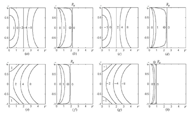
Figure 1: Magnetic field lines and density contours for pure primordial magnetic flux at the horizontal edges, $M=0$: (a-b) $B=-1$, $I^{(0)}=2$, $I^{(1)}=1$, $\phi^{(1)}=0.5$, $R_{d}\approx 2.2$; (c-d) $B=1$, $I^{(0)}=2$, $I^{(1)}=-1$, $\phi^{(1)}=-0.5$, $R_{d}\approx 2.3$; (e-f) $B=1$, $I^{(0)}=2$, $I^{(1)}=1$, $\phi^{(1)}=-0.5$, $R_{d}\approx 1.9$; (g-h) $B=-1$, $I^{(0)}=2$, $I^{(1)}=-1$, $\phi^{(1)}=0.5$, $R_{d}\approx 1$.

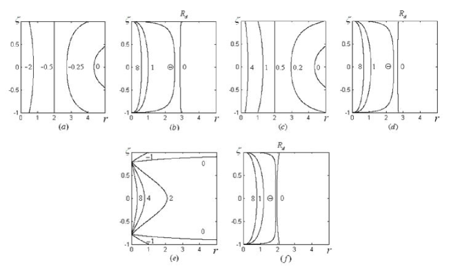
Figure 2: Magnetic field lines and density contours for pure dipole magnetic flux at the horizontal edges, $B=0$: (a-b) $M=1$, $I^{(0)}=0.5$, $I^{(1)}=1$, $\phi^{(1)}=-1$, $R_{d}\approx 2.9$; (c-d) $M=-1$, $I^{(0)}=0.5$, $I^{(1)}=-1$, $\phi^{(1)}=1$, $R_{d}\approx 2.7$; (e-f) $M=1$, $I^{(0)}=0.5$, $I^{(1)}=-2$, $\phi^{(1)}=-0.5$, $R_{d}\approx 2$.

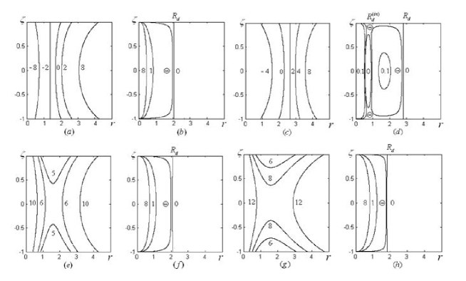
Figure 3: Magnetic field lines and density contours for mixed magnetic flux at the horizontal edges: (a-b) $M=4$, $B=1$, $I^{(0)}=2$, $I^{(1)}=1$, $\phi^{(1)}=-0.5$, $R_{d}\approx 2$; (c-d) $M=4$, $B=1$, $I^{(0)}=2$, $I^{(1)}=-1$, $\phi^{(1)}=-0.5$, $R_{d}\approx 2$; (e-f) $M=-4$, $B=1$, $I^{(0)}=2$, $I^{(1)}=-1$, $\phi^{(1)}=-0.5$, $R_{d}\approx 2$; (g-h) $M=-4$, $B=1$, $I^{(0)}=2$, $I^{(1)}=1$, $\phi^{(1)}=-0.5$, $R_{d}\approx 1.9$.

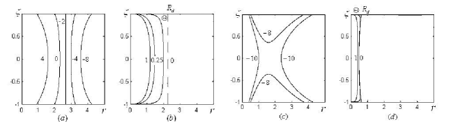
Figure 4: Magnetic field lines and density contours for mixed magnetic flux at the horizontal edges: (a-b) $B=-1$, $M=-4$, $I^{(0)}=2$, $I^{(1)}=1$, $\phi^{(1)}=-0.5$, $R_{d}\approx 2.2$; (c-d) $B=-1$, $M=4$, $I^{(0)}=2$, $I^{(1)}=-1$, $\phi^{(1)}=-0.5$, $R_{d}\approx 0.5$.

.

5.2 Numerical examples for the second family of equilibrium solutions (Figs. 5-8)

For the second family of equilibrium solutions the density is given by a pure hydrodynamic Keplerian distribution (see Fig. 5), and it is the same for all admissible magnetic field configurations in Figs. 6-8 (with parameters $M$, $B$, $I^{(0)}$ scaled by $\delta$, and restricted to $\phi^{(1)}>0$). To illustrate the qualitative behavior of the magnetic field, the field lines of the scaled magnetic flux $\psi_{1}(r,\zeta)=[\psi(r,\zeta)-\delta\Gamma(r)]/\delta$ are depicted in Figs. 6, 7 and 8 for different kinds of the edge magnetic flux: with zero dipole-moment, pure dipole-like magnetic field and mixed magnetic fields.

The second family of equilibria generates structures that are quite similar to those in the first family, e.g. X-points in Figs. 6c, 6d, 8f, 8g, 8h, and several configurations with a single O-point structures in Figs. 6a, 6b, 7b, 8c, 8d. In addition, new kinds of the structures arise and may be seen in Figs. 7a,7c, 7d and Fig. 8a, 8b, 8e. Thus, Figure 7c demonstrates a magnetic island with radius that increases infinitely with decreasing magnetic flux value. Then double O-point structures appears with magnetic islands additional to those centered on the O-point at the coordinate origin. Figures 7a, 7d and 8e demonstrate presence of two magnetic islands (”plasmoids”), first with central O-points located at the origin of the coordinate, and second with both finite radius of magnetic islands and coordinate of O-point inside the disk in Fig. 8e, or with both the radius of magnetic island and coordinate of O-point which tend to infinity in Figs. 7a and 7d. Figures 8a and 8b with a single O-points located at the origin separated from the right by a separatrix $\psi_{1}=0$ demonstrate the magnetic lines with strong variations of their gradients from the right of the separatrix. Figure 8e demonstrates the presence of O-points, closed magnetic lines confined both from the left and right by the separatrix $\psi_{1}=0$, while X-points are in Figs. 8f-8h. Finally note that some of the equilibrium magnetic lines obtained above are quite similar to the instantaneous magnetic lines obtained experimentally in a tokomak (e.g. Fig. 6 in Iisuka et al. (1986)).

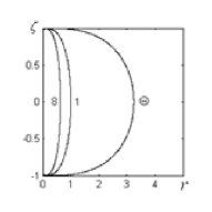
Figure 5: Density contours for the second family of solutions.

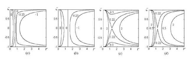
Figure 6: Perturbed magnetic field lines for pure primordial magnetic flux at the horizontal edges, $M=0$ , $\phi^{(1)}=1$: (a) $B=-1$, $I^{(0)}=1$, $I^{(1)}=-1$; (b) $B=-1$, $I^{(0)}=1$, $I^{(1)}=1$; (c) $B=1$, $I^{(0)}=1$, $I^{(1)}=1$; (d) $B=1$, $I^{(0)}=1$, $I^{(1)}=-1$.

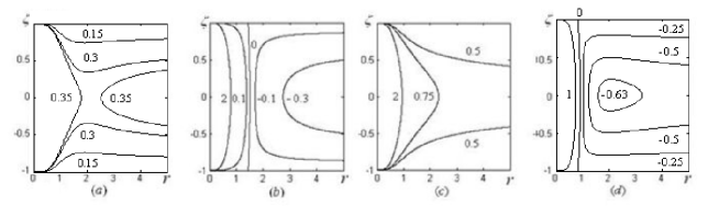
Figure 7: Perturbed magnetic field lines for pure dipole magnetic flux at the horizontal edges, $B=0$, $\phi^{(1)}=1$: (a) $M=1$, $I^{(0)}=1$, $I^{(1)}=1$; (b) $M=-1$, $I^{(0)}=1$, $I^{(1)}=-1$; (c) $M=-1$, $I^{(0)}=1$, $I^{(1)}=1$; (d) $M=1$, $I^{(0)}=1$, $I^{(1)}=-1$.

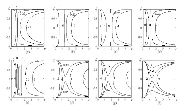
Figure 8: Perturbed magnetic field lines for mixed magnetic flux at the horizontal edges, $\phi^{(1)}=1$: (a) $B=-1$, $M=1$, $I^{(0)}=1$, $I^{(1)}=-1$; (b) $B=-1$, $M=1$, $I^{(0)}=1$, $I^{(1)}=1$; (c) $B=-1$, $M=-1$, $I^{(0)}=1$, $I^{(1)}=1$; (d) $B=-1$, $M=-1$, $I^{(0)}=1$, $I^{(1)}=-1$; (e) $B=1$, $M=1$, $I^{(0)}=1$, $I^{(1)}=-1$; (f) $B=1$, $M=1$, $I^{(0)}=1$, $I^{(1)}=1$; (g) $B=1$, $M=-1$, $I^{(0)}=1$, $I^{(1)}=-1$; (h) $B=1$, $M=-1$, $I^{(0)}=1$, $I^{(1)}=1$.

6 SUMMARY AND DISCUSSION

3D axially-symmetric steady-state equilibria of weakly ionized polytropic Hall-MHD plasmas are investigated for the Keplerian portion of thin disks. Asymptotic expansions in small aspect ratio $\epsilon$ provide an efficient way to construct an equilibrium model for differentially rotating disks. There are three principle Hall equilibrium states which can not be reduced from one to the other, classified according to the following orientations of the magnetic field lines: (i) pure toroidal, (ii) pure poloidal, and (iii) mixed toroidal and poloidal equilibria. The three classes of equilibria differ from each other by the different ordering with respect to $\epsilon$ of the various components of the magnetic field. In the present study the most interesting case is investigated that involves both toroidal and poloidal components of the magnetic field that are of the same zero order in $\epsilon$. The disk structure is described by the GS equation for the poloidal flux that involves two arbitrary functions $I(\psi)$ and $\phi(\psi)$ for the toroidal electric current and electric potential, respectively. The arbitrariness of functions $I(\psi)$ and $\phi(\psi)$ in steady-state problems reflects the uncertainty of the initial data in the general initial value problem. The flux function is symmetric about the midplane and satisfies certain boundary conditions at the horizontal edges of the disk (radial variations of the disk height are neglected). The boundary conditions for the magnetic flux $\psi=\Gamma(r)$ at the horizontal disk edges express the joint effect of an primordial magnetic field, and a dipole-like magnetic field that reflects the influence of the central body on the Keplerian disk. Solutions for different configurations of the magnetic field and density are obtained explicitly for trial linear approximations of the current $I(\psi)=I^{(0)}+I^{(1)}\psi$ flowing through a circular area in a plane and of the electric potential $\phi(\psi)=\phi^{(1)}\psi$ (where $I^{(0)}$ is the total current concentrated along the disk axis), as well as several forms of the boundary magnetic flux $\Gamma(r)$.

A particular noteworthy new feature of the present model is the finite radius of the rotating disks which is inherent for the Hall equilibrium. By using a small parameter $\delta$ proportional to the inverse Hall parameter with a small coefficient of proportionality, it is established that the Hall equilibria disks fall into two types which are characterized by quite different orders in $\delta$: Keplerian disks with (i) small ($R_{d}\sim\delta^{0}$) and (ii) large (${R_{d}}\gtrsim\delta^{-k}$, $k>0$) radius of the disk. For disks of the first family a finite radius of the disk appears as a cut-off value at which the plasma density vanishes. Disks of the second family have large (finite or infinite) radii due to non-uniformity of the asymptotic expansions in $\delta$.

The method developed here allows to investigate analytically the equilibrium states with a large number of possible combinations of boundary conditions for the magnetic flux. Thus, it is demonstrated that all possible mutual orientations of the rotating axis, the primordial magnetic field, and the magnetic moment of the central body, as well as the relative strength of the two latter give rise to a great richness of possible topologies of the magnetic field lines. Such configurations includes geometries with O-points, with X-points, with material gaps and rings, with detached plasmoids, with magnetic islands, and with zero net induced magnetic flux. Note that magnetic islands centered on O-points are typical for steady-state equilibria in Keplerian disk. For instance they have been simulated in thin disk approximation within MHD model for the pure poloidal magnetic field (Lovelace et al. (1986)). On the other hand, equilibria that contain X-points are more subtle and generally have a strong tendency to undergo a significant change in their topology due to possible reconnection processes (Priest & Forbes (2000)). The latter however is commonly speculated to be responsible for widely observed astrophysical phenomena like jets and winds. Describing such processes requires an extensive stability analysis. Since the primordial poloidal flux on the disk is likely too small to be responsible for the observed total magnetic flux in disk systems (Colgate and Li 2001), the possible flux enhancing due to instability of axisymmetric Hall equilibria becomes an important issue. Additionally, it is natural then to incorporate multipoles of higher odd orders (Lepeltier and Aly 1999) instead of the primordial poloidal flux, in addition to the dipole adopted here, into to the boundary flux sources at the origin that describe the central object effect on the Keplerian disk. The stability study of the developed equilibrium disks may provide further selection of admissible magnetic configurations. For instance, development of X-point configurations may lead to an instability of such equilibria, since X-point equilibrium solutions are rather structurally unstable and a small perturbation of the equilibrium likely leads to an essential change in its form, such as magnetic lines reconnection and transition to the neighborhood stable (smooth) configuration. The present Hall equilibrium solution for thin Keplerian disks may be incorporated to the leading order in small aspect ratio into a more sophisticated problem accounting for accretion and jet inflow (similar to Ogilvie 1997).

References

- Balbus & Terquem (2001) Balbus, S. A., & Terquem, C., 2001, ApJ, 552, 235
- Bogoyavlenskij (2000) Bogoyavlenskij, O. I., 2000, Physique math matique/Mathematical Physics, C. R. Acad. Sci. Paris, 331, 569
- Brandenburg et al. (1995) Brandenburg, A., Nordlund, A., Stein, R.F., & Torkelsson, U., 1995, ApJ, 446, 741
- Calvet et al. (2002) Calvet, N., D’Alessio, P., Hartmann, L., Wilner, D., Walsh, A., & Sitk, M., 2002, ApJ, 568, 1008
- Colgate & Li (2000) Colgate, S. A., & Li H., 2000, Highly Energetic Physical Processes and Mechanisms for Emission from Astrophysical Plasmas, IAU Symposium, P. C. H., eds., Martens and S. Tsuruta, 195, 255 (San Francisco: ASP)
- Coppi & Keyes (2003) Coppi B., & Keyes, E.A., 2003, ApJ, 595, 1000
- Desch (2004) Desch S. J., 2004, ApJ, 608, 509
- Fromang & Papaloizou (2007) Fromang, S., & Papaloizou, J., 2007, A&A, 476, 1113
- Fromang et al. (2002) Fromang, S., Terquem, C. & Balbus, C.A., 2002, MNRAS, 329, 18
- Gammie (1996) Gammie, C.F., 1996, ApJ., 457, 355
- Hawley & Krolik (2002) Hawley, J. F., & Krolik, J. H., 2002, ApJ, 566, 164
- Huba (1991) Huba, J. D., 1991, Phys. Fluids B, 3, 3217
- Iisuka et al. (1986) Iisuka, S., Minamitani, Y., & Tanaka, H., 1986, Plasma Phys. and Contr. Fusion, 28, 973
- Kaiser & Lortz (1995) Kaiser, R., & Lortz, D., 1995, Phys. Rev. E, 52, 3034
- Kluzniak & Kita (2000) Kluzniak, W., & Kita, D., 2000, astro-ph/0006266.
- Kolberg et al. (2005) Kolberg, Z., Liverts, E., & Mond, M., 2005, Phys. Plasmas, 12, 062113
- Hayashi et al. (1985) Hayashi, C., Nakazawa, K., & Nakagawa, Y., 1985, in Protostars and Planets II, eds. D.C. Black & M.S. Mathews, University of Arizona Press, Tucson
- Igea & Glassgold (1999) Igea, J., & Glassgold, A.E., 1999, ApJ., 518, 848
- Lepeltier & Aly (1996) Lepeltier, T., & Aly, J.J., 1996, A&A, 306, 645
- Liverts & Mond (2004) Liverts, E., & Mond, M., 2004, Phys. Plasmas, 11, 55
- Liverts & Mond (2008) Liverts, E., & Mond, M., 2009, MNRAS, 392, 287
- Lovelace et al. (1986) Lovelace R. V. E., Mehanian C., Mobarry C.M., & Sulkanen M.E., 1986, ApJ, 62, 1
- Lovelace et al. (2002) Lovelace R. V. E., Li H., Koldoba A. V., Ustyugova G. V., & Romanova M. M., 2002, ApJ, 572 445
- Matt et al. (2002) Matt S., Goodson A.P., Winglee R. M., & Bohm K.-H., 2002, ApJ, 574 232
- McClements & Thyagaraja (2001) McClements, K. G., & Thyagaraja, A., 2001, MNRAS, 323 733
- Ogilvie (1997) Ogilvie, G. I., 1997, MNRAS, 288, 63
- Pandey & Wardle (2008) Pandey, B. P., & Wardle M., 2008, MNRAS, 385, 2269
- Papaloizou & Terquem (1997) Papaloizou, J. C. B., & Terquem C., 1997, MNRAS, 287, 771
- Priest & Forbes (2000) Priest, E. R., & Forbes, T., 2000, Magnetic Reconnection - MHD Theory and Applications, (Cambridge: University Press)
- Proga (2003) Proga D., 2003, ApJ, 585 406
- Regev ( 1983) Regev, O., 1983, A&A, 126, 146
- Rudiger & Kitchatinov (2005) Rdiger, G., & Kitchatinov, L.L., 2005, A&A, 434, 629
- Salmeron & Wardle (2003) Salmeron, R., & Wardle, M., 2003, MNRAS, 345, 992
- Salmeron & Wardle (2005) Salmeron, R., & Wardle, M., 2005, MNRAS, 361, 45
- Sano & Stone (2002) Sano, T., & Stone, J., 2002, MNRAS, 570, 314
- Shtemler et al. (2007) Shtemler, Y. M., Mond., M., & Liverts., E., ApJ, 665, 1371
- Thyagaraja & McClements (2006) Thyagaraja A. and McClements K. G., 2006, Phys. Plasmas, 13, 062502
- Terquem & Papaloizou (1996) Terquem, C., & Papaloizou, J. C. B., 1996, MNRAS, 279, 767
- Umebayashi & Nakano (1988) Umebayashi T., & Nakano, T., Prog. Theor. Phys. Suppl., 96, 151
- Umurhan et al. (2006) Umurhan, O. M., Nemirovsky, A., Regev, O., & Shaviv, G., A&A, 446, 1
- Urpin & Rudiger (2005) Urpin, V., & Rdiger, G., 2005, A&A, 437, 23
- Wardle (1999) Wardle M.,199, MNRAS,307,849
- Wu & Chen (1989) Wu, H., & Chen Y., 1989, Phys. Fluids B 1, 1753