Mountain trail formation and the active walker model

Abstract

We extend the active walker model to address the formation of paths on gradients, which have been observed to have a zigzag form. Our extension includes a new rule which prohibits direct descent or ascent on steep inclines, simulating aversion to falling. Further augmentation of the model stops walkers from changing direction very rapidly as that would likely lead to a fall. The extended model predicts paths with qualitatively similar forms to the observed trails, but only if the terms suppressing sudden direction changes are included. The need to include terms into the model that stop rapid direction change when simulating mountain trails indicates that a similar rule should also be included in the standard active walker model.

PACS Nos.: 89.65.-s, 89.40.-a, 89.75.Kd

1 Introduction

The dynamics of pedestrians and their interactions with the environment have become a central theme in the study of social physics [6]. An aspect of pedestrian dynamics that has received considerable attention is the description of spontaneously formed trail systems. Unexpected patterns can be found in trail systems, highlighting the interplay between effective attractions and itinerancy when walking from a starting point to a destination [7]. The creation of powerful models of human trail formation could help to improve planning and understanding of paths and related phenomena [7, 9, 8, 10, 4, 5]. However, we are not aware of any physics based studies of the formation of mountain trail systems, where poor planning for human activity can lead to significant environmental damage [2, 3].

In principle, there are a huge number of possible routes to be explored when choosing a path, and walkers could take any course between a starting point and a destination. A first approximation to the most probable path is a straight line between the initial and destination points (unless there are obstacles in the way). However, studies of trails using the active walker model have shown that the detailed patterns of paths form from a counterpoint between the desire to walk on well trodden paths, and the shortest route to be found by traveling directly between the origin and destination [7, 9]. Well-trodden paths are likely to be favored by pedestrians because of reduced energy usage when compared, for example, to walking through long grass. This preference may be largely psychological, as internet based experiments in a virtual environment have also shown that ‘walkers’ tend to favor well-used ‘paths’ [4, 5]. The preference to walk on regularly used paths leads to an effective interaction between past and present walkers, indicating that there is interesting physics involved in the formation of such trails.

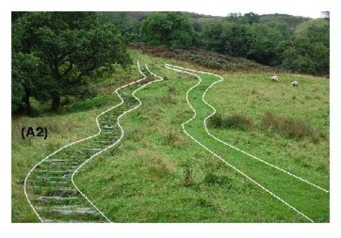
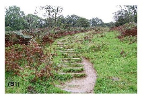
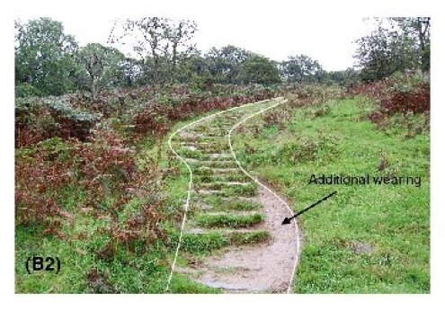
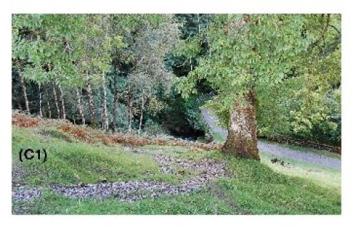
Figure 1: (Color online) Spontaneously formed zig-zag paths on Wansfell, near Ambleside, Lake District, Cumbria, UK. (A1, A2) The left hand path has been augmented by humans since its formation. The right hand path is spontaneously formed in the grass. Both paths have a similar angle relative to the steepest direction and regularity of direction change.). (B1, B2) Another zigzag path from further up the trail. Recent wearing of the path can be seen. The top paths are on inclines of around 1:8. The bottom path (figures C1, C2) is on a much steeper incline of around 1:2. This path was found close to Low Sweden Bridge near Ambleside, and breaks off from the main path that can be seen curving around towards the back of the picture. White lines are included on the right hand versions of the figures to highlight the paths.

On inclines, there is a third influence. Walkers may ascend slopes diagonally if the gradient of the incline becomes too steep to ascend directly. Walking at an angle to the line of fastest ascent has the effect of decreasing the effective gradient of the incline, permitting travel up steeper slopes. On descent, it may not be possible to walk directly down a very steep slope without becoming unbalanced, again leading walkers to take a diagonal path. Our aim in this article is to determine if the walkers’ desire to avoid steep gradients, in combination with the rules of the active walker model, can be used to simulate the zigzag paths that can be observed in mountainous regions.

The energetics of walking on an incline have been discussed by Alexander in a simple model of bipedal locomotion [1]. From energy considerations, walkers aim to change the angle of ascent from the vertical if a hill reaches a steep enough gradient. In Ref. alexander2002a, human walkers are omniscient, and are able to assess the energetic outlay for an entire route. In this way, they can assess if more energy would be expended taking a shallower and longer route, or if a quick hike up a steep route would be more favorable. We consider that it is unlikely that the information about all possible routes is available for global decisions to influence route and planning, and expect that decisions are more likely to be local. Moreover, modeling has concluded that humans choose well trodden paths in a more local manner [8]. We therefore consider that insight into mountain trail formation could be gained from active walker simulations of inclined planes.

To demonstrate some examples of paths on inclines, we took photographs in the Lake District in Cumbria, England, which can be seen in Fig. 1. The upper panels Fig. 1(A1,A2) show spontaneously formed zig-zag paths on Wansfell. Two paths can be seen to the left and right hand sides of the picture, as highlighted in the figure on the right (A2). The left hand path has been augmented with rock since its formation, but still shows the characteristic zig-zag. To remove doubt on the origin of the zig-zags (for example, the stones might have been laid according to a plan) a second path can be seen to the right of the picture. The right hand path is spontaneously formed in the grass. Both have similar path angle and regularity of direction change. An example from further up the trail can be seen in panels B1 and B2. Here, there is additional wear to the side of the trail, indicating that the trail is still evolving. The paths are on inclines of around 1:8. The bottom path (C1 and C2) is on an incline of around 1:2, and was observed near Low Sweden Bridge which is close to the village of Ambleside. Trails of this type are not unique to England, and such paths can be seen in other locations, such as Smith Rock in the USA, where the bends in the paths are large enough to appear on trail maps [14].

This article continues as follows. We review the rules of the active walker model in section 2. In section 3 we briefly discuss aspects of the biomechanics of walking on inclines. Extensions of the active walker model for mountain trail systems are introduced in section 4. Results of simulations are shown in section 5. Finally we summarize in section 6.

2 Active walker model for human trails

In order to investigate trail formations on mountains we use a modified form of the active walker model, which was introduced in Refs. helbing1997a and helbing1997b. In this section, we review the rules of the unmodified active walker model following the scheme introduced in Ref. helbing1997a. Since the active walker model forms the basis of our extension to mountain trails, it is our aim to ensure that all specific features of the active walker model are clear, before introducing our extensions to the model in section 4.

The aim of the active walker model is to describe the formation of paths in soft ground. As pedestrians walk on soft surfaces such as grass, the ground becomes worn and a path emerges. In the active walker model, the wear on the soft surface is assumed to be represented by a function, $G(\boldsymbol{r},t)$, which represents the ground condition at time $t$ and position $\boldsymbol{r}$. As is common in statistical physics, $G(\boldsymbol{r},t)$ is assumed to evolve according to a first-order rate equation,

$$\frac{{\rm d}G({\boldsymbol{r}},t)}{{\rm d}t}=\frac{1}{T}\left[G_{0}-G({\boldsymbol{r}},t)\right]+I\left[1-\frac{G({\boldsymbol{r}},t)}{G_{\rm max}}\right]\sum_{\mu}\delta({\boldsymbol{r}}-{\boldsymbol{r}}_{\mu}).$$ (1)

The rate of change of $G(\boldsymbol{r},t)$ depends on weathering (the first term on the right hand side of the equation) and wear by walkers (the second term). The rate of weathering is governed by the parameter $1/T$, where $T$ sets the time scale of path decay back to the undisturbed ground condition $G_{0}$. The saturation value is denoted $G_{\rm max}$. The parameter controlling the damage caused by a footprint is denoted $I$. Walkers are located at positions ${\boldsymbol{r}}_{\mu}$, and $\delta({\boldsymbol{r}})$ is the Dirac delta function. In the presence of more than one walker, $\mu$ is an index corresponding to the walker being considered. Note that $G$ is a positive quantity in this study.

The Dirac $\delta$-function found in equation 1 is not especially convenient to use for numerics. Therefore, we suggest the following small modification to equation 1,

$$\frac{{\rm d}G({\boldsymbol{r}},t)}{{\rm d}t}=\frac{1}{T}\left[G_{0}-G({\boldsymbol{r}},t)\right]+I\left[1-\frac{G({\boldsymbol{r}},t)}{G_{\rm max}}\right]\sum_{\mu}f({\boldsymbol{r}}-{\boldsymbol{r}}_{\mu}).$$ (2)

where $f({\boldsymbol{r}}-{\boldsymbol{r}}_{\mu})$ is an arbitrary function that specifies the shape of the damage caused by a footfall. $f({\boldsymbol{r}})$ is normalized to unity. We take $f$ to be a square with sides $l=10$cm long, i.e. to have similar area to the base of a shoe. With this choice of $f$, $l^{2}G_{\rm max}/I$ is the approximate number of footfalls that cause $G$ to reach the saturation value $G_{\rm max}$. Since the feet of walkers have finite dimensions, we consider equation 2 to be more physical than equation 1.

The positions of the walkers are updated according to how attracted they are to any local paths, and the direction of the destination. Each walker $\mu$ is influenced by a potential that depends on their location relative to the paths. The attraction of local paths is determined from,

$$V({\boldsymbol{r}}_{\mu},t)=\int{\rm d}^{2}{\boldsymbol{r}}\exp\left(-|{\boldsymbol{r}}-{\boldsymbol{r}}_{\mu}|/\sigma\right)G({\boldsymbol{r}},t).$$ (3)

The exponential function indicates how visible the path at ${\boldsymbol{r}}$ is to the pedestrian at location ${\boldsymbol{r}}_{\mu}$. The parameter, $\sigma$ controls the distance over which walkers are motivated to make detours to well formed trails. We note that the sign of the potential $V$ is opposite to the usual convention, i.e. a positive $V$ indicates an attraction. There are no negative $V$, since $G$ is always positive. This is in agreement with the sign convention used in Ref. helbing1997b.

There are two competing influences on walkers in the active walker model. The first is the desire to reach the destination in as direct a manner as possible. In the conventional active walker model, each walker with index $\mu$ aims for a destination point, $\boldsymbol{d}_{\mu}$. In the absence of any paths, it is reasonable to expect walkers to travel by the most direct route, i.e. along the unit vector $(\boldsymbol{d}_{\mu}-\boldsymbol{r}_{\mu})/|\boldsymbol{d}_{\mu}-\boldsymbol{r}_{\mu}|$. The attractive potential defined in equation 3 generates an effective force in the same direction as the gradient of the potential $\nabla_{\boldsymbol{r}_{\mu}}V(\boldsymbol{r}_{\mu},t)$. In the active walker model, $\nabla_{\boldsymbol{r}_{\mu}}V(\boldsymbol{r}_{\mu},t)$ and $(\boldsymbol{d}_{\mu}-\boldsymbol{r}_{\mu})/|\boldsymbol{d}_{\mu}-\boldsymbol{r}_{\mu}|$ are both used to define the direction $\boldsymbol{e}$ that walker $\mu$ moves along from position $\boldsymbol{r}_{\mu}$ in the presence of a set of paths,

$$\boldsymbol{e}(\boldsymbol{r}_{\mu},t)=\frac{(\boldsymbol{d}_{\mu}-\boldsymbol{r}_{\mu}(t))/|{\boldsymbol{d}}_{\mu}-{\boldsymbol{r}}_{\mu}(t)|+\nabla_{r_{\mu}}V_{\mu}(\boldsymbol{r}_{\mu},t)}{|(\boldsymbol{d}_{\mu}-\boldsymbol{r}_{\mu}(t))/|{\boldsymbol{d}}_{\mu}-{\boldsymbol{r}}_{\mu}(t)|+\nabla_{r_{\mu}}V_{\mu}({\boldsymbol{r}}_{\mu})|}$$ (4)

$\nabla_{r_{\mu}}V({\boldsymbol{r}}_{\mu},t)$ is the direction of favorable ground. The symbol $\nabla_{r_{\mu}}$ represents the gradient of $V$ taken with respect to the position vector of the walker $\boldsymbol{r}_{\mu}$ (the subscript acts as a reminder that the gradient is not taken with respect to $\boldsymbol{r}$). $\boldsymbol{e}$ is a dimensionless unit vector.

The active walker model is completed with the equation of motion,

$$\frac{{\rm d}{\boldsymbol{r}}_{\mu}}{{\rm d}t}=v_{0\mu}{\boldsymbol{e}}({\boldsymbol{r}}_{\mu},t)$$ (5)

where $v_{0\mu}$ is the walking speed of walker $\mu$, assumed to be constant for the entire journey of the walker. In the discretized form of the equations, $v_{0\mu}$ is related to the length of a stride.

The active walker model has been successful in describing some of the unexpected features that have been observed in trail systems. The application of the active walker model to the winding paths found on steep inclines has not yet been considered. In the following section, we discuss the biomechanics of walking on inclined planes with the aim of developing additional rules to explain the wiggles observed in trail systems on hills.

3 The biomechanics of walking on inclines

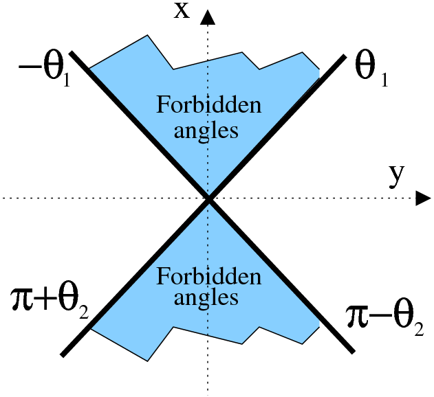
Figure 2: Schematic of the region of discomfort for walking up or down the mountain. If the active walker model suggests angles in the shaded area $|\gamma|<\theta$, the angle will be mapped to either $\theta$ or $-\theta$ depending on which side of the axis the optimally desired angle lies. The mapping also depends on whether the walker is going up or down the incline. We estimate that a forbidden angle of around $10^{o}$ corresponds to a $1:4$ gradient. Note that the $x$-axis is defined to be in the direction directly up the gradient, and the $y$ axis along the contour of no height change. Angles are defined from the $x$-axis.

In this section, we aim to give a brief summary of the physiological factors that must be considered when modeling walkers on inclined planes. Some insight into the manner of walking that is adopted on an incline can be gained from attempts to develop bipedal robots that can climb sloping surfaces [16]. If exactly the same method is used to climb a slope as to walk on flat paths, the center of gravity is positioned further back than usual, which may lead to a fall [16] (a good introduction to the biomechanics of walking on flat surfaces can be found in Ref. whittle2001a). Humans (and robots developed to climb slopes) compensate for the effects of the slope by leaning forward, which can be achieved by flexing the ankle. This is satisfactory for very shallow slopes. However, if a slope is too steep, it becomes physiologically impossible to turn the ankle joint through the angle necessary to hold the center of gravity over the feet (for example, the person investigated in Ref. leroux2002a could not bend his/her ankle by more than 24^o). Thus good foot contact cannot be maintained with the ground when walking directly up very steep inclines.

Experiments have shown that the requirements on joints increase dramatically on moderate slopes [11, 12]: walking on a 10^o incline requires hip flexibility of 60^o, compared with 30^o on the flat. Demands on ankle flexibility increase in a similar way. Joints in the leg such as the ankle, knee and hip are also subjected to significantly increased forces [12]. As determined in Ref. leroux2002a, the ankle becomes fully bent for more of the walking cycle as the gradient increases from $0^{o}$ to $10^{o}$. The physiological constraints on the angles through which joints can bend indicate that hills eventually become too steep to walk up directly. To compensate for the limits of joint flexibility, the walker can choose to change the angle of ascent, to avoid walking directly uphill. This leads to a smaller effective gradient. The inability to walk directly uphill can be thought of as an effective potential barrier against certain walking directions.

There is also a risk of falling on descent. This is probably greater than the chance of falling on ascent, since parts of the walking cycle require the center of gravity to be moved forward [15] and on descent, the body is already unstable to falling forwards. Again, it is possible to compensate against falling by reducing the angle of descent. As before, we expect this compensation to lead to an effective potential barrier for angles that are likely to cause a fall (most walkers will have learned to avoid tumbling). When simulating mountain trails it is important to include this behavior.

There is an additional feature of walking that should be relevant regardless of whether the walker is on an incline or level ground. Given the constraints of anatomy, sudden changes of direction between consecutive footsteps are likely to lead to discomfort, instability, falling or significant reduction in speed. Rapid changes of direction correspond to significant changes in the momentum of the walker and therefore large forces are required to maintain stability. These forces are applied at ground level, so can lead to a significant torque on the walker and toppling. We therefore expect walkers to have a preference to make consecutive footsteps in similar directions. We now describe the inclusion of incline effects and the inability to make sudden changes of direction into the active walker model.

4 A model of mountain walkers

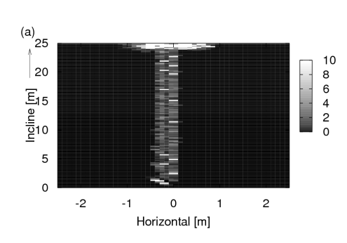
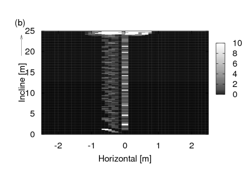
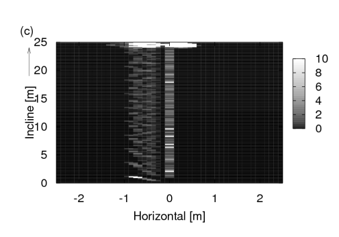
Figure 3: Ground condition for (a) $\theta=15^{o}$ (b) $\theta=25^{o}$ and (c) $\theta=35^{o}$. In all cases, the persistence of direction $\alpha=0$. If consecutive steps are not taken in similar directions, no clear zig-zag paths form.

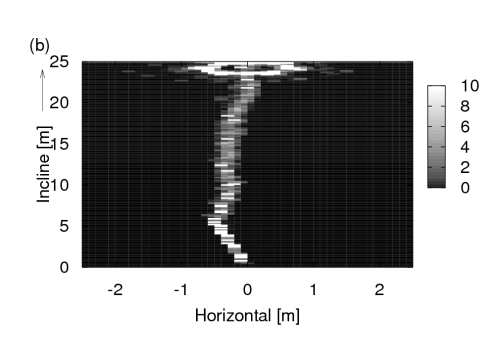
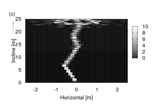
Figure 4: Ground condition for simulations with minimum safe angle $\theta=5^{o}$ and persistence of direction (a) $\alpha=0.4$ (b) $\alpha=0.5$ and (c) $\alpha=0.6$. As the tendency to make consecutive footfalls in the same direction increases, the size of the features increases.

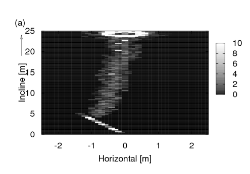
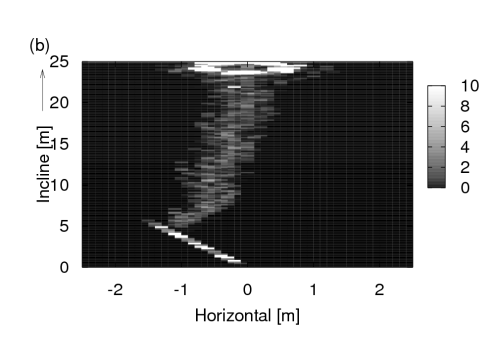
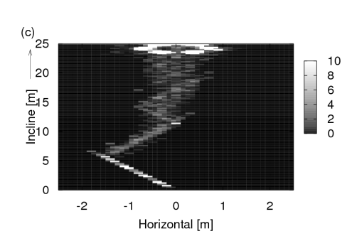
Figure 5: Ground condition for simulations with $\theta=15^{o}$ and (a) $\alpha=0.4$ (b) $\alpha=0.45$ and (c) $\alpha=0.5$.

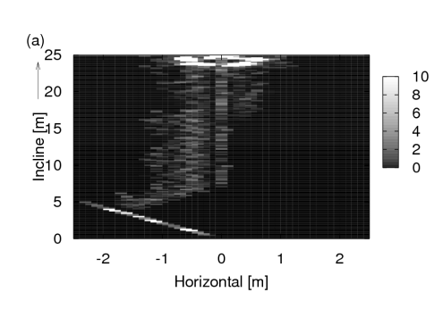
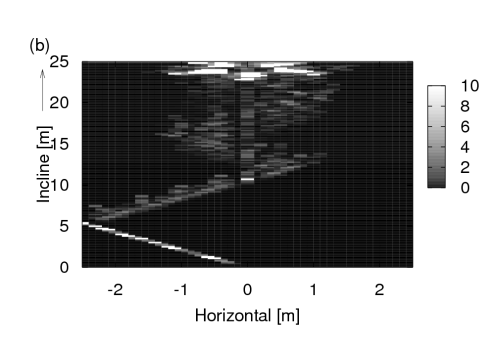
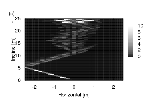
Figure 6: Ground condition for simulations with $\theta=25^{o}$ and (a) $\alpha=0.4$ (b) $\alpha=0.45$ and (c) $\alpha=0.5$.

4.1 New rules for mountain walking

It is our aim extend the active walker model to construct a “mountain walker model”. As we have discussed in section 3, our model should take account of the inability of walkers on steep inclines to walk directly up or down a slope if the gradient becomes too great, and avoid sudden changes of direction that can cause instability.

We suggest two ways of implementing an aversion to sudden changes in direction:

Rule Ia

The new direction of the walker is taken as the weighted average of the recent angle of motion $\phi$ and the angle of motion that would be favored on a flat surface.

$$\gamma(t)=\alpha\phi+(1-\alpha)\beta(t),$$ (6)

We call the parameter $\alpha$ the persistence of direction. $\beta$ is the angle that is determined from the direction vector $\boldsymbol{e}=e_{x}\boldsymbol{i}+e_{y}\boldsymbol{j}$,

$$\beta(t)=\tan^{-1}(e_{y}(t)/e_{x}(t))$$ (7)

where $\boldsymbol{i}$ and $\boldsymbol{j}$ are unit vectors in the $x$ (uphill) and $y$ (horizontal) directions respectively. In the determination of $\beta$, care is taken to ensure that the angle is in the quadrant consistent with the signs of $e_{x}$ and $e_{y}$. We take care to avoid any problems with branch cuts in equations 6 and 7. Strictly, $\phi$ should relate to the direction of the walker over the time period just before

$$\phi=\int_{t-\Delta}^{t}\beta(t^{\prime}){\rm d}t^{\prime}/\Delta$$ (8)

where $\Delta$ is the time period within which the direction of previous footsteps is relevant to stability.

We also suggest an alternative to equation 6.

Rule Ib

Equation 2 is supplemented with the average direction over recent time,

$$\boldsymbol{e}(\boldsymbol{r}_{\mu},t)=\frac{(\boldsymbol{d}_{\mu}-\boldsymbol{r}_{\mu}(t))/|{\boldsymbol{d}}_{\mu}-{\boldsymbol{r}}_{\mu}(t)|+\nabla_{r_{\mu}}V_{\mu}(\boldsymbol{r}_{\mu})+\frac{\bar{\alpha}}{\Delta}\int_{t-\Delta}^{t}\boldsymbol{e}(\boldsymbol{r}_{\mu},t^{\prime}){\rm d}t^{\prime}}{|(\boldsymbol{d}_{\mu}-\boldsymbol{r}_{\mu}(t))/|{\boldsymbol{d}}_{\mu}-{\boldsymbol{r}}_{\mu}(t)|+\nabla_{r_{\mu}}V_{\mu}({\boldsymbol{r}}_{\mu})+\frac{\bar{\alpha}}{\Delta}\int_{t-\Delta}^{t}\boldsymbol{e}(\boldsymbol{r}_{\mu},t^{\prime}){\rm d}t^{\prime}|}.$$ (9)

where again $\Delta$ is the time within which sudden change of direction would lead to falling and $\bar{\alpha}$ is a parameter that controls the influence of the previous footsteps.

We also modify the active walker model to incorporate the potential barrier in angle space that represents the inability to achieve a safe journey if the walker is traveling too close to the directly uphill or downhill routes (i.e. a journey where the walker is unlikely to fall over). This rule is summarized in figure 2.

Rule IIa

(To be used with rule Ia) If the angle $\gamma$, chosen from equation 6, falls within a forbidden zone ($|\gamma|<\theta$), the angle along which the walker moves is mapped to the nearest minimum angle of safety (either $\theta$ or $-\theta$). We assume that the larger the incline of the slope, the larger the region of angles that are not permitted. This is equivalent to having an infinite effective potential barrier in certain directions. In the event that $\gamma=0$ our walker has a preference to move left. If there is a mapping, we reconstruct $\boldsymbol{e}$ from $\gamma$ as $\boldsymbol{e}=\cos(\gamma)\boldsymbol{i}+\sin(\gamma)\boldsymbol{j}$, noting that the sense of $\boldsymbol{i}$ is up the plane. The new $\boldsymbol{e}$ is then used to update the position of the walker via eqn. 5.

Rule IIb

(To be used with rule Ib) If the angle, $\beta=\tan^{-1}(e_{y}/e_{x})$, lies within a forbidden zone ($|\beta|<\theta$), then the vector $\boldsymbol{e}$ is mapped to the closest angle outside the forbidden region. If $\beta=0$ the walker moves left. Since $\beta=0$ on the first iteration, our paths show a bias in that direction.

4.2 Discretization scheme

We use the following simple first-order discretization procedure to solve the active walker model and extensions. The time coordinate is discretized into small intervals $\Delta t$, and the spatial coordinates into intervals $\Delta x$ and $\Delta y$. Therefore, the vector $\boldsymbol{r}$ can be written in the discrete form ${\boldsymbol{r}}=(\eta\Delta x,\nu\Delta y)$ where $\eta$ and $\nu$ are integers. Approximated using this scheme, equation 2 becomes,

$$G({\boldsymbol{r}},t_{n}):=G({\boldsymbol{r}},t_{n-1}) + \frac{\Delta t}{T}\left[G_{0}-G({\boldsymbol{r}},t_{n-1})\right]$$ (10)

$$+\sum_{\mu}I\Delta t\left[1-\frac{G({\boldsymbol{r}},t_{n-1})}{G_{\rm max}}\right]f_{(}{\boldsymbol{r}}-{\boldsymbol{r}}_{\mu}(t_{n-1})),$$

The integral in equation 3 becomes a sum, so the potential can be computed as,

$$V_{\mu}({\boldsymbol{r}},t_{n}):=\sum_{\eta,\nu}\Delta x\Delta ye^{-|{\Delta x\eta\boldsymbol{i}+\Delta y\nu\boldsymbol{j}}-{\boldsymbol{r}}_{\mu}(t_{n-1})|/\sigma}G({\Delta x\eta\boldsymbol{i}+\Delta y\nu\boldsymbol{j}},t_{n}),$$ (11)

From the potential, the direction of the walker $\boldsymbol{e}$ can be computed. For convenience, we will write the numerator of eqn. 4 as the un-normalized vector $\bar{\boldsymbol{e}}$, and then normalize it once it has been computed to calculate $\boldsymbol{e}$. The un-normalized $x$-component of eqn. 4 becomes,

$$\bar{e}_{x\mu}(t_{n}):=\frac{(d_{x}-r_{x})}{|{\boldsymbol{d}}-{\boldsymbol{r}}|}+\frac{[V_{\mu}(x_{\mu}+\Delta x,y_{\mu})-V_{\mu}(x_{\mu}-\Delta x,y_{\mu})]}{2\Delta x},$$ (12)

and the unnormalized $y$-component of eqn. 4 is approximately,

$$\bar{e}_{y\mu}(t_{n}):=\frac{(d_{y}-r_{y})}{|{\boldsymbol{d}}-{\boldsymbol{r}}|}+\frac{[V_{\mu}(x_{\mu},y_{\mu}+\Delta y)-V_{\mu}(x_{\mu},y_{\mu}-\Delta y)]}{2\Delta y},$$ (13)

Here $x_{\mu}$ and $y_{\mu}$ are defined via $\boldsymbol{r}_{\mu}=x_{\mu}\boldsymbol{i}+y_{\mu}\boldsymbol{j}$. The components $\bar{e}_{x\mu}$ and $\bar{e}_{y\mu}$ are combined into a single vector $\bar{\boldsymbol{e}}=\bar{e}_{x\mu}\boldsymbol{i}+\bar{e}_{y\mu}\boldsymbol{j}$ which is then normalized to determine the direction of the next step,

$${\boldsymbol{e}}(t_{n}):=\bar{{\boldsymbol{e}}}(t_{n})/|\bar{{\boldsymbol{e}}}(t_{n})|$$ (14)

The average angle (equation 8) is approximately,

$$\phi=\sum_{i=1}^{\Delta/\Delta t}\beta(t_{n-i})\Delta t/\Delta$$ (15)

with a similar scheme for the average of previous directions in equation 9. Equation 9 is otherwise discretized in the same way as equation 12.

The walker position is updated according to the discretized version of eqn. 5.

$${\boldsymbol{r}}_{\mu}(t_{n}):={\boldsymbol{r}}_{\mu}(t_{n-1})+\Delta tv_{0}{\boldsymbol{e}}_{\mu}(t_{n}).$$ (16)

The vectors ${\boldsymbol{r}}_{\mu}$ were permitted to take any real value to avoid truncation errors that could lead to limit cycles.

It is important to note that, in general, the validity of first order integration schemes is not guaranteed. We checked our code and approximate scheme against results in Refs. helbing1997a and helbing1997b, finding no significant differences. We have run simulations using 3 different resolutions of $\Delta x$, $\Delta y$ and $\Delta t$ (see the results section of this article). The scheme was found to converge quickly on reduction of the size of the discrete steps.

As humans tend to walk with different step sizes, we varied the speed of the individual walkers. This variation leads to continuous paths. The width of the area studied was chosen as 10m and the length of the observed area (in the direction of the incline) as 25m. This is probably realistic for this type of trail formation, since we suspect that walkers aim for local goals, rather than the final goal of the peak (which is not necessarily visible from all locations).

4.3 Algorithm one

To clarify our computational scheme further, we detail the algorithms that we use for computation. Two computational schemes have been used. Algorithm one is based on Rules Ia and IIa, with algorithm two based on Rules Ib and IIb. The steps in the algorithm are:

1. To initialize, set the ground condition to the default value $G(\boldsymbol{r},t_{0})=0$.

2. Choose a walker speed following equation $v_{0\mu}=(0.5+r)$ms^-1, where $r$ is a random number between 0 and 1.

3. Select the direction for the walker (i.e. up or down-hill) randomly with equal probability.

4. Initialize the walker position at the bottom or top of the incline depending on whether an up or down walker has been selected.

5. Compute the attractive potential $V$ from equation 11.

6. Determine the default walker direction from equation 14.

7. Apply the persistence of direction formula, equation 6

8. Apply the forbidden angle rule. If the angle, $\gamma$, lies within a forbidden zone ($|\gamma|<\theta$), then the vector $\boldsymbol{e}$ is mapped to the closest angle outside the forbidden region. In the event that $\gamma=0$ our walker has a preference to move left.

9. Update the walker position using equation 16.

10. Update the ground condition using equation 10.

11. Repeat from step 5 until the walker has reached the destination.

12. Repeat from step 2 until the action of sufficient walkers on the ground condition has been investigated.

4.4 Algorithm two

1. Initialize the ground condition.

2. Select the speed of the walker.

3. Select the direction of the walker.

4. Initialize the walker position.

5. Compute $V$ from equation 11.

6. Apply the alternative formula for persistence of direction, equation 9.

7. Apply the forbidden angle rule. If the angle, $\beta$, lies within a forbidden zone ($|\beta|<\theta$), then the vector $\boldsymbol{e}$ is mapped to the closest angle outside the forbidden region. In the event that $\gamma=0$ our walker has a preference to move left.

8. Update the walker position $\boldsymbol{r}_{\mu}$ using equation 16.

9. Update $G$ using equation 10.

10. Repeat from step 5 until the destination has been reached.

11. Repeat from step 2 until the desired number of walkers have traversed the slope.

The simulation was implemented in c++. The random number generator, ran2 from ‘Numerical Recipes in C’ was used to ensure a long period [13]. We tested our code against the triangular and square examples in Ref. helbing1997b.

5 Results

5.1 Algorithm one

In this section, results from the mountain walker extension to the active walker model are shown. We begin by considering only walkers traveling down the slope. The following parameters were used for the simulations: the maximum ground potential was set to $G_{\rm max}=200$m^-1 (the units of $G$ are set by Eq. 3 and Eq. 4) while the minimum ground potential was set to $G_{0}=0$. Larger values of $G_{\rm max}$ lead to larger attraction to the path. A new walker descended the inclined area as soon as the existing walker reached the destination (tests showed that there was little difference between this scheme and starting a walker every 100s). The visibility, $\sigma$ of the paths was set to 10m and the intensity, $I$ was set to $l^{2}G_{\rm max}/N$, where $N$ is the number of footprints needed to wear the ground condition to $1/e$ of its maximum value. $N$ was set to 50 footfalls and the weathering parameter was initially set to $T=1000$s. The values of $N$ and $T$ are smaller than in a real trail system, where $N$ would be of the order of several hundred footfalls and $T$ would be of the order of a few days. This still leads to realistic simulations since Helbing et al. have found that a combination of several parameters of the active walker model could be represented by the single parameter $\kappa=IT/\sigma=G_{\max}T/N\sigma$ [7]. Individual walkers were assigned a random speed between 0.5m/s and 1.5m/s. In the simulation, walkers were given the starting position ${\boldsymbol{r}}_{\rm initial}=(0{\rm m},5{\rm m})$ and a destination of ${\boldsymbol{r}}_{\rm final}=(25{\rm m},5{\rm m})$ with the $x$-direction being the distance down the incline and $y$-direction the distance across the incline. Initially, 25000 walkers traversed the incline in each simulation.

In our initial simulations, we set the parameter $\alpha=0$, consistent with the standard setup of the active walker model. This led to a curious result, as shown in Fig. 3. We found that walkers changed their walking direction frequently, with some walkers changing direction on every time step. This waddling gait is not very comfortable on an incline, and it is likely to make the walker very unstable. Also, the speed of advance down a hill is likely to be quite slow. We thoroughly investigated the parameter space to look for the zigzag paths, but did not find them. As this waddling gait is not a practical way to descend a mountain, it is reasonable to conclude that the active walker model is missing some crucial physics: a walker is much more likely to ambulate by moving consecutive legs in similar directions, otherwise the resulting motion will be very unstable. For this reason, we introduce a factor, $\alpha$, to represent persistence of direction (see Eq. 6). $\alpha$ controls a weighted average between the angles on consecutive time steps.

By changing the weighting factor, which alters the influence of the recent direction of motion on the walker, and by changing the size of the forbidden angle $\theta$, we were able to estimate how large $\alpha$ needs to be to produce convincing zigzag paths. Again, we assumed that walkers always traveled down the incline (in the direction of increasing $x$) and otherwise used the same parameters. We ran simulations with $\theta$ ranging from $\theta=5^{o}$ to $\theta=45^{o}$ and $\alpha$ ranging from $\alpha=0.1$ to $\alpha=0.9$.

We show the results of single runs for a minimum safe angle of $\theta=5^{o}$ in figure 4. The zig-zag paths are immediately apparent. Multiple turns in the path can be seen when the parameter, $\alpha\gtrsim 0.5$ (Fig. 4(b)). This indicates that when walkers choose where to place the next footfall, around half of the choice comes from a desire to maintain the previous walking direction, and half from the wish to reach the destination quickly via a path. The effect of reducing the influence of the previous angle can be seen in Fig. 4(a) where $\alpha=0.4$. As a result of the reduced influence of the previous direction, the walker’s motion follows only a slight wiggle. In panel (c) of Fig. 4, where $\alpha=0.6$ and the influence of the previous angle is increased, the overall size of features increases. This is a common feature of all simulations where the influence of previous step directions is increased through $\alpha$.

As the minimum safe angle is increased to $15^{o}$, we note that the minimum values of $\alpha$ which are needed to generate zig-zag patterns decreases slightly. In Fig. 5(a) where $\alpha=0.4$, we observe that a single zigzag emerges in the path. As walkers get closer to their destination, the rate at which they change their walking direction increases. Fig. 5(b) shows a similar path for $\alpha=0.45$. In Fig. 5(c) we observe that when $\alpha=0.5$ walkers take larger detours away from the direct path between entry and exit, with several changes of direction along the trail. Similar results were found when $\theta=25^{o}$ (Fig. 6). While zigzag forms develop during the simulations, the rather diffuse paths are not satisfactory representations of mountain trails.

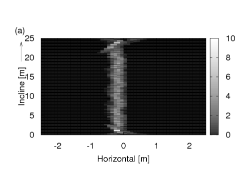
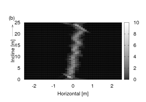
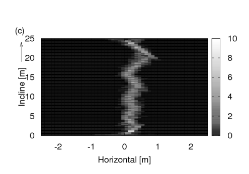
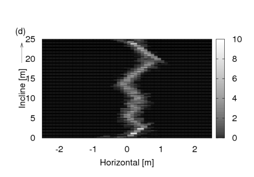
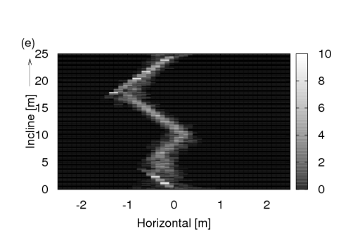
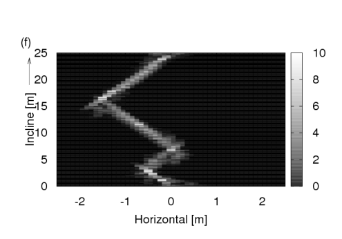
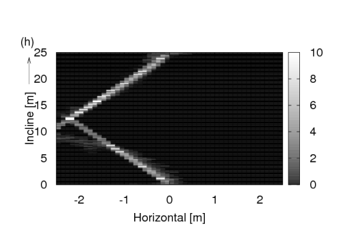
Figure 7: The results of simulations of 2500 walkers traveling consecutively up and down the incline. Algorithm one is used (a) $\alpha=0.30$ (b) $\alpha=0.35$ (c) $\alpha=0.40$ (d) $\alpha=0.45$ (e) $\alpha=0.50$ (f) $\alpha=0.55$ (g) $\alpha=0.60$ (h) $\alpha=0.65$. $T=1500$s, $N=50$, $\sigma=10$m and $v=(0.5+r)$ms^-1 where $r\in[0,1)$ is a random variate. We also considered simulations with 25000 walkers, with no noticeable difference to the pattern of paths formed. $\Delta t=1.0$s

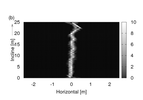
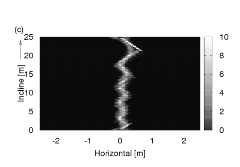
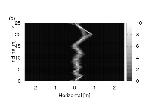
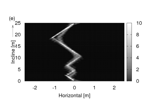
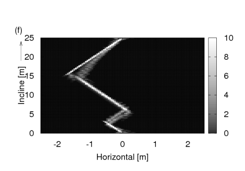
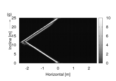
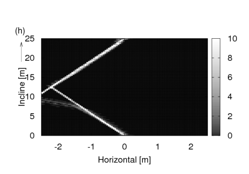
Figure 8: As Fig. 7 with double the space and time resolution used in the computation $\Delta x=\Delta y=5$cm and $\Delta t=0.5$s. The shapes of the paths are robust against the finite size scaling.

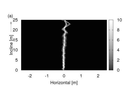
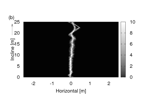
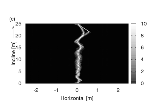
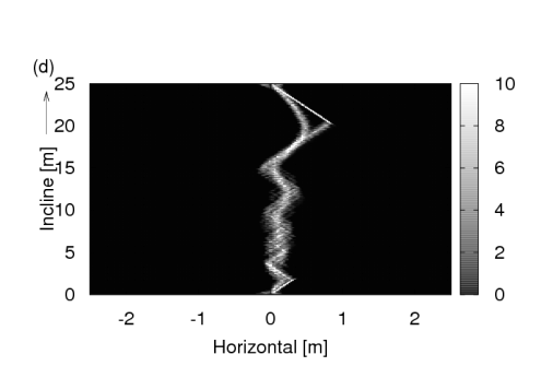
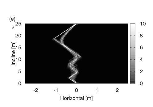
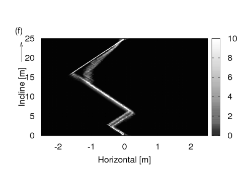
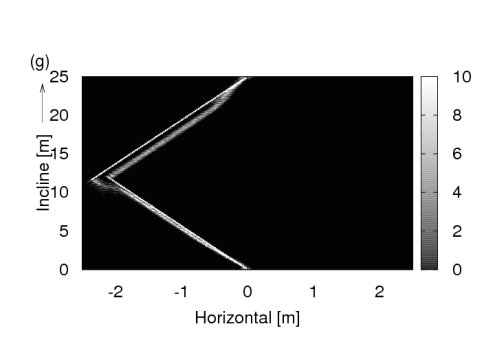
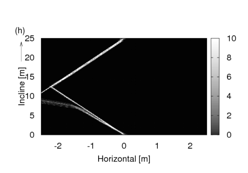
Figure 9: As Fig. 7 with four times the space and time resolution used in the computation $\Delta x=\Delta y=2.5$cm and $\Delta t=0.25$s. Again, the shapes of the paths are robust against the finite size scaling.

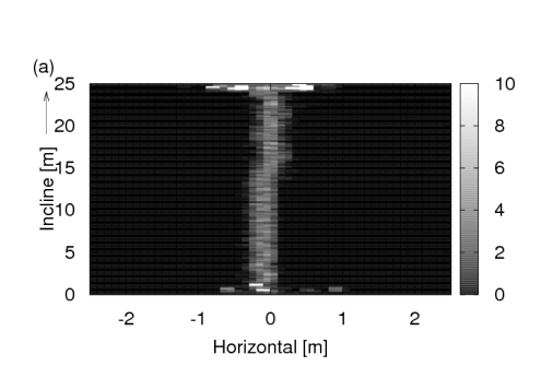
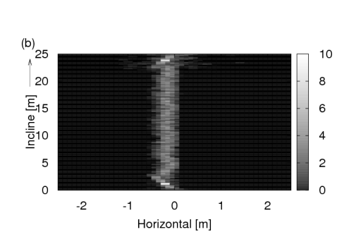
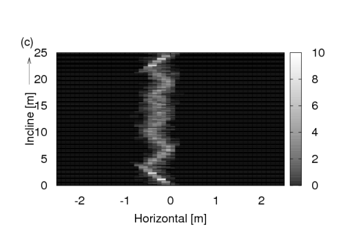
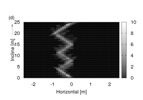
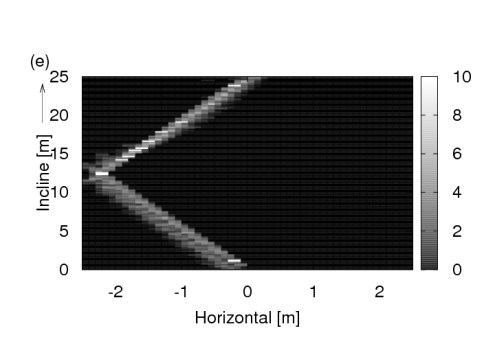
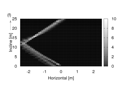
Figure 10: The alternative direction averaging scheme for the mountain walker. (a) $\bar{\alpha}=0.5$, (b) $\bar{\alpha}=1.0$, (c) $\bar{\alpha}=1.5$, (d) $\bar{\alpha}=2.0$, (e) $\bar{\alpha}=2.5$, (f) $\bar{\alpha}=3.0$. $\Delta t=1$s, $\Delta x=\Delta y=10$cm. Results from both schemes are in qualitative agreement. The size of features increases monotonically with $\bar{\alpha}$.

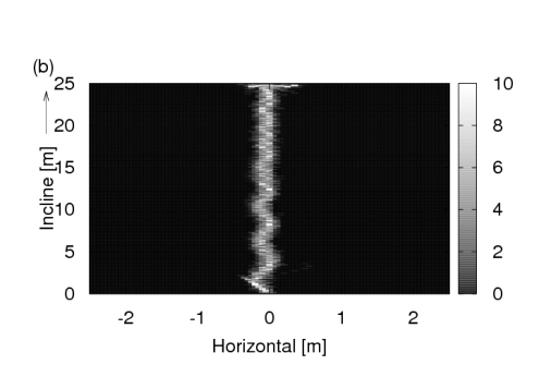
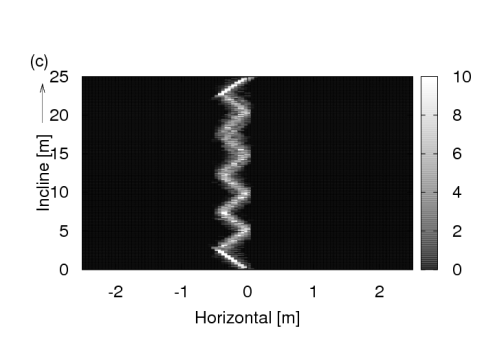
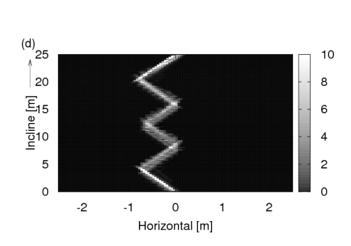
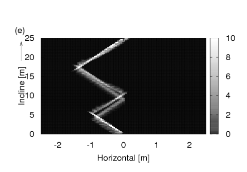
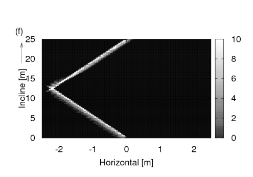
Figure 11: As figure 10, except $\Delta t=0.5$s, $\Delta x=\Delta y=5$cm.

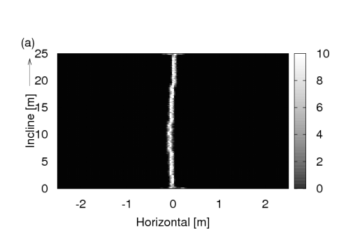
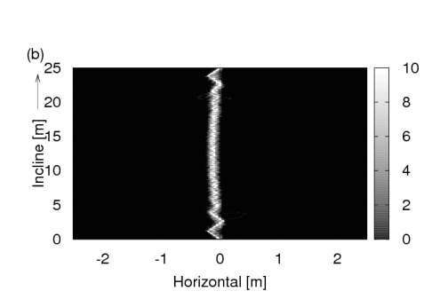
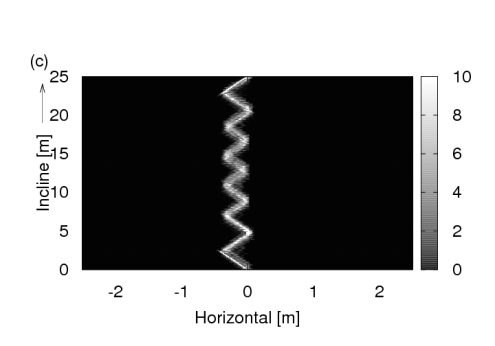
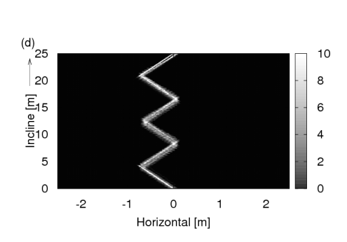
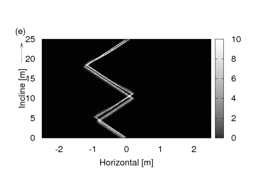
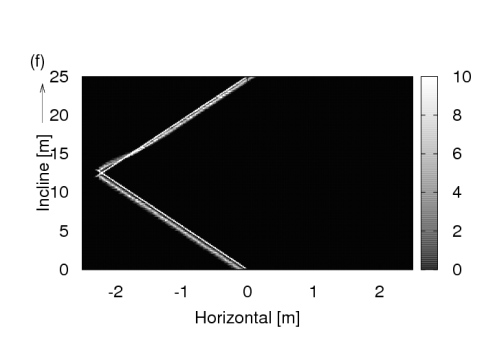
Figure 12: As figure 10, except $\Delta t=0.25$s, $\Delta x=\Delta y=2.5$cm.

We complete our simulations using algorithm one, by examining walkers that travel consecutively up and down the incline. Results of the simulations can be seen in figure 7. A slightly different weathering time of $T=1500$s was used. There is no requirement that the forbidden angles are the same for hikers moving up and down the incline. In general, we expect that the different mechanisms for walking up and down inclines lead to different forbidden angles. In this set of simulations, we choose a forbidden angle of $\theta_{1}=25^{o}$ for walkers moving up the diagram (down the gradient). Those moving down the diagram (up the gradient) have a minimum safe angle of $\theta_{2}=10^{o}$. We run simulations for a range of $\alpha$. Some zig-zag patterns can be seen for low alpha, but patterns of decent size do not appear until $\alpha\gtrsim 0.45$ (panel d), Again, the sizes of the bends in the path increase in size with $\alpha$. The combined effect of walkers moving in both directions are trails with zig-zag patterns that have a similar angle to the largest of the two forbidden angles. The walkers with a smaller forbidden angle round off the sharp turns in the paths that were found on the zig-zags formed when walkers are only permitted to move in a single direction. This rounding is a direct consequence of the attraction term in the active walker model and may explain the curved nature of spontaneously formed mountain trails. Moreover, the inclusion of walkers with different minimum safe angles leads to well defined trails (rather than the diffuse trails found previously). This is probably because the walkers with smaller forbidden angles have more freedom to change direction, allowing the active walker rules to function effectively.

To test the effects of discretization, we compute results using smaller $\Delta t=0.5$s, $\Delta x=5$cm and $\Delta y=5$cm in figure 8. In figure 9 we use even smaller steps $\Delta t=0.25$s, $\Delta x=2.5$cm and $\Delta y=2.5$cm. The absence of new features shows our calculations to be stable against finite size scaling.

5.2 Algorithm two

We also run simulations using algorithm two. The results are shown in Figs. 10, 11 and 12 with the resolution of the discretization increased between figures. 2500 walkers traversed the incline in both directions. The parameters of the runs were $T=1500$s, $N=50$, $\sigma=10$m and $v_{0\mu}=(0.5+r)$ms^-1 where $r\in[0,1)$ is a random variate. $\bar{\alpha}$ was varied. Again, we choose $\theta_{1}=25^{o}$ and $\theta_{2}=10^{o}$. The results from both algorithms one and two are in good qualitative agreement. Note that the results for $\bar{\alpha}=2.5$ required slightly higher resolution for convergence. In comparison to the patterns from algorithm one, the zigzags are quite regular. Small wiggles of around $0.5$metres across form when $\bar{\alpha}=1.5$. As before, the features become larger as $\bar{\alpha}$ is increased.

6 Summary

We have developed an extension to the active walker model to handle the formation of trails on inclines. Our simulations are in qualitative agreement with empirical observations of mountain path formations. Such trails are characterized by a zig-zag pattern. Our extension took account of the inability of walkers to walk directly up or down very steep gradients. We have shown that some supplementary rules need to be included in the active walker model to achieve features consistent with mountain trails. Those additional rules are that (a) the consecutive steps of walkers tend to be in the same direction and that (b) there is a maximum permitted angle of motion down an incline to avoid falling and (c) there is a maximum angle of ascent for physiological reasons such as limited ankle flexibility. When rules to encourage consecutive steps are not present, we find that walkers travel in an unusual manner, only taking a single step before changing direction. We also found that the presence of walkers moving both uphill and downhill (with different forbidden angles) is important for forming well defined zig-zag paths. Walkers traveling downhill with a larger forbidden angle are constrained to form zigzags but create rather diffuse paths unless those paths are complemented by walkers traveling uphill. This happens because the walkers with more angular freedom become attracted to and reinforce the paths.

The preference of walkers to take consecutive steps in the same direction could also be relevant for the understanding of trail formation in flat areas, and it is our opinion that a persistence of direction parameter should also be included when simulating trail systems on level ground. Thus, our main conclusions are that (1) correlation between consecutive step directions should be included in the active walker model and that (2) an extension of the active walker model to include forbidden angles, correlation between consecutive steps and the combination of walkers moving both up- and down-hill is suitable to understand the formation of mountain paths.

References

- [1] R. M. Alexander. Am. J. Hum. Biol., 14:641, 2002.
- [2] K. L. Bell and L. C. Bliss. Biological Conservation, 5:25, 1973.
- [3] R. Coleman. Applied Geography, 1:121, 1981.
- [4] R. L. Goldstone, A. Jones, and M. E. Roberts. IEEE Transactions on Systems, Man and Cybernetics, Part A, 36:611, 2006.
- [5] R. L. Goldstone and M. E. Roberts. Complexity, 11:43, 2006.
- [6] D. Helbing. Rev. Mod. Phys., 73:1067, 2001.
- [7] D. Helbing, J. Keltsch, and P. Molnar. Nature, 388:47, 1997.
- [8] D. Helbing, P. Molnar, I. Farkes, and K. Bolay. Environment and Planning B: Planning and Design, 28:361, 2001.
- [9] D. Helbing, F. Schweitzer, J. Kelysch, and P. Molnar. Phys. Rev. E, 56:2527, 1997.
- [10] A. Kirchner, H. Klupfel, K. Nishinari, A. Schadschneider, and M. Schreckenberg. J. Stat. Mech, 2004:P10011, 2004.
- [11] A. Leroux, J. Fung, and H. Barbeau. Gait and Posture, 15:6474, 2002.
- [12] A. S. McIntosh, K. T. Beatty, L. N. Dwan, and D. R. Vickers. Journal of Biomechanics, 39:2491, 2006.
- [13] W. H. Press, S. A. Teukolsky, W. T. Vetterling, and B. P. Flannerty. Numerical Recipes in C: The art of Scientific Computing. Cambridge University Press, 1992.
- [14] A. Watts. Climber’s guide to Smith rock. Falcon Guides, Guilford, CT, USA, 1992.
- [15] M. W. Whittle. Gait analysis: An introduction. Butterworth-Heinemann Ltd., 2001.
- [16] Y. F. Zheng and J. Shen. IEEE Transactions on Robotics and Automation, 6:86, 1990.