Preferred numbers and the distribution of trade sizes and trading volumes in the Chinese stock market
Abstract
The distribution of trade sizes and trading volumes are investigated based on the limit order book data of 22 liquid Chinese stocks listed on the Shenzhen Stock Exchange in the whole year 2003. We observe that the size distribution of trades for individual stocks exhibits jumps, which is caused by the number preference of traders when placing orders. We analyze the applicability of the ``-Gamma'' function for fitting the distribution by the Cramér-von Mises criterion. The empirical PDFs of trading volumes at different timescales ranging from 1 min to 240 min can be well modeled. The applicability of the -Gamma functions for multiple trades is restricted to the transaction numbers . We find that all the PDFs have power-law tails for large volumes. Using careful estimation of the average tail exponents of the distribution of trade sizes and trading volumes, we get , well outside the Lévy regime.
pacs:
89.65.GhEconomics; econophysics, financial markets, business and management and 89.75.DaSystems obeying scaling laws and 89.75.-kComplex systems1 Introduction
A well-known adage says: It takes volume to move stock prices, indicating that the trade size and trading volume contain much information about the dynamics of price formation. The topic of price-volume relationship has a long history in finance Karpoff-1987-JFQA and recently has been investigated at the transaction level Chan-Fong-2000-JFE ; Lillo-Farmer-Mantegna-2003-Nature ; Lim-Coggins-2005-QF ; Naes-Skjeltorp-2006-JFinM ; Zhou-2007-XXX . Furthermore, understanding the origin of power-law tails in returns is an important issue. In the unified theory of Gabaix et al Gabaix-Gopikrishnan-Plerou-Stanley-2003-Nature , the power-law tails of returns are related to the power-law tails of volumes, where the institutional activity plays a crucial role Gabaix-Gopikrishnan-Plerou-Stanley-2006-QJE ; Gabaix-Gopikrishnan-Plerou-Stanley-2007-JEEA ; Gabaix-Gopikrishnan-Plerou-Stanley-2008-JEDC . Zhou verified the relation at the transaction level, although the values of exponents are remarkably different from those of Gabaix et al Zhou-2007-XXX . On the other hand, Farmer et al have found that large price changes at the transaction level are driven by liquidity fluctuations rather than by volume Farmer-Gillemot-Lillo-Mike-Sen-2004-QF . In particular, they showed that the return distribution is closely related to the distribution of gaps between the first two price levels on the order book. Webber and Rosenow argued that large stock price fluctuations can be explained quantitatively by taking into account both the order flow and the liquidity Weber-Rosenow-2006-QF . In addition, Joulin et al also found that most price jumps are induced by order flow fluctuations close to the point of vanishing liquidity and volume plays a minor role Joulin-Lefevre-Grunberg-Bouchaud-2008-XXX . In any case, the distributions of trading volume are of interest, also as part of stylized facts.
The issue of the tail distribution of trade sizes is also controversial. The probability density function of trade sizes has a fat tail often described by a power law:
| (1) |
Gopikrishnan et al analyzed the transaction data for the largest 1000 stocks traded on the three major US markets and found that the distribution of trade sizes follows a power-law tail with the exponent being , and called this as the half-cubic law Gopikrishnan-Plerou-Gabaix-Stanley-2000-PRE ; Plerou-Gopikrishnan-Gabaix-Amaral-Stanley-2001-QF ; Plerou-Gopikrishnan-Gabaix-Stanley-2004-QF . The aggregated trading volumes at timescales from a few minutes to several hundred minutes were found to have a power-law tail exponent Gopikrishnan-Plerou-Gabaix-Stanley-2000-PRE ; Plerou-Gopikrishnan-Gabaix-Amaral-Stanley-2001-QF ; Plerou-Gopikrishnan-Gabaix-Stanley-2004-QF 111It is noteworthy to point out that Farmer and Lillo investigated three LSE stocks and found no clear evidence for power-law tails Farmer-Lillo-2004-QF .. Maslov and Mills also found that the trade sizes of several NASDAQ stocks have power-law tails with the exponent close to 1.4 Maslov-Mills-2001-PA . Plerou and Stanley extended this analysis to other two markets (LSE and Paris Bourse) and found quantitatively similar results across the three distinct markets Plerou-Stanley-2007-PRE . All these tail exponents were found to be well below 2, within the Lévy regime.
Alternatively, Eisler and Kertész reported that the tail exponents of the traded volumes at a timescale of 15 minutes for six NYSE stocks are 2.2 and 2.8 Eisler-Kertesz-2006-EPJB ; Eisler-Kertesz-2007-PA . Racz, Eisler and Kertész argued that the tail exponents of the trade size were underestimated Racz-Eisler-Kertesz-2008-XXX . They investigated the 1000 most liquid stocks traded on the NYSE for the same period as studied by Plerou and Stanley Plerou-Stanley-2007-PRE and found that the average tail exponent is . The tail exponents were found to be outside the Lévy regime for stocks in the Korean stocks Lee-Lee-2007-PA and the Chinese stocks Zhou-2007-XXX .
The above mentioned studies concern with the tail behavior of the trade size or trading volume distribution. There are also efforts attempting to describe the whole distribution of trading volumes. The normalized trading volumes of 10 top-volume NYSE stocks and NASDAQ stocks at different timescales of 1 min, 2 min and 3 min were fitted by the -Gamma distribution Tsallis-Anteneodo-Borland-Osorio-2003-PA
| (2) |
where
| (3) |
is the normalization constant, and are positive parameters, and the value of is larger than 1. The usage of the -Gamma distribution can be motivated from a stochastic dynamical scenario Queiros-2005-EPL ; deSouza-Moyano-Queiros-2006-EPJB ; Queiros-Moyano-deSouza-Tsallis-2007-EPJB . In the limiting case 1, the traditional Gamma probability density function is recovered. The asymptotic behavior of the -Gamma distribution has a power-law form (Eq. (1)) with
| (4) |
Compared with Eq. (1), we find the asymptotic tail exponent
| (5) |
Here, we use to make the difference between the empirical tail exponent and the fitting one. From the results of reference Queiros-2005-EPL , we find the tail exponent is greater than 2 for 10 high-volume NASDAQ stocks (for which and are available) at different timescales of 1 min and 2 min.
In this paper, we focus on investigating the distributions of trade sizes and trading volumes, based on limit order book data of 22 liquid stocks. The trade size is defined as the number of shares exchanged in trade , and trading volume is defined as the share volumes in a fixed time interval. Here we consider two types of trading volumes based on different definitions of the time interval, event time and clock time. The first one is defined as the total volume traded in a fixed clock-time interval :
| (6) |
where is the number of transactions in a fixed interval . The second one is defined as the total volume traded in a fixed event-time interval :
| (7) |
where is the number of trades. The issue of trade sizes is a special case when . Our work deals with the problem of describing the whole distributions and with the estimation of the tail exponent.
2 Description of the data
We used tick by tick data for 22 liquid stocks traded on the Shenzhen Stock Exchange (SZSE) in the whole year 2003. The market consists of three time periods on each trading day, namely, the opening call action (9:15 AM to 9:25 AM), the cooling period (9:25 AM to 9:30 AM), and the continuous double auction (9:30 AM to 11:30 AM and 1:00 PM to 3:00 PM). In this paper, we consider only the transactions occurring in the double continuous auction. The size of each transaction is recorded in the data sets. In the Chinese stock market, the size of a buy order is limited to a board lot of 100 shares or an integer multiple thereof, while a seller can place a sell order with any size. The recorded trade size is in units of shares.
The tickers of the 22 stocks investigated are the following: 000001 (Shenzhen Development Bank Co. Ltd: 887,741 trades), 000002 (China Vanke Co. Ltd: 509,360 trades), 000009 (China Baoan Group Co. Ltd: 447,660 trades), 000012 (CSG holding Co. Ltd: 290,148 trades), 000016 (Konka Group Co. Ltd: 188,526 trades), 000021 (Shenzhen Kaifa Technology Co. Ltd: 411,326 trades), 000024 (China Merchants Property Development Co. Ltd: 133,586 trades), 000027 (Shenzhen Energy Investment Co. Ltd: 313,057 trades), 000063 (ZTE Corporation, 265,450 trades), 000066 (Great Wall Technology Co. Ltd: 277,262 trades), 000088 (Shenzhen Yan Tian Port Holdings Co. Ltd: 97,195 trades), 000089 (Shenzhen Airport Co. Ltd: 189,117 trades), 000429 (Jiangxi Ganyue Expressway Co. Ltd: 117,424 trades), 000488 (Shandong Chenming Paper Group Co. Ltd: 120,097 trades), 000539 (Guangdong Electric Power Development Co. Ltd: 114,721 trades), 000541 (Foshan Electrical and Lighting Co. Ltd: 68,737 trades), 000550 (Jiangling Motors Co. Ltd: 346,176 trades), 000581 (Weifu High-Technology Co. Ltd: 93,947 trades), 000625 (Chongqing Changan Automobile Co. Ltd: 397,393 trades), 000709 (Tangshan Iron and Steel Co. Ltd: 207,756 trades), 000720 (Shandong Luneng Taishan Cable Co. Ltd: 132,233 trades), and 000778 (Xinxing Ductile Iron Pipes Co. Ltd: 157,321 trades).
The 22 stocks investigated in this work cover a variety of industry sectors such as financials, real estate, conglomerates, metals & nonmetals, electronics, utilities, IT, transportation, petrochemicals, paper & printing and manufacturing. Our sample stocks were part of the 40 constituent stocks included in the Shenshen Stock Exchange Component Index in 2003 Zhou-2007-XXX .
Note that when we investigate trading volumes and of all 22 stocks, we have normalized the trade sizes by the total number of outstanding shares to account for share splits.
3 Trade size distribution
3.1 Trade size distribution of individual stocks
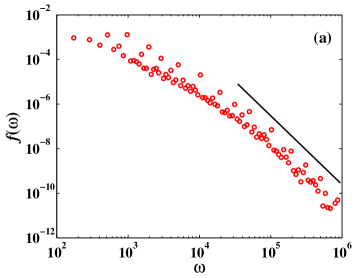
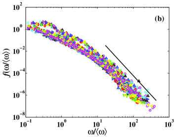
In this section, we study the trade size distribution of individual stocks. Fig. 1(a) displays the probability density function (PDF) of a typical stock (Shenzhen Development Bank Co., LTD, code 000001) and Fig. 1(b) shows the PDFs of the normalized trade sizes of 22 stocks, where is the mean trade size for individual stocks. The most intriguing feature is that the PDFs are not continuous and there are evident jumps in the curves. The outliers seem rather equidistant on the log scale. The reason is that the traders seem to have a sense of number preference, which will be discussed in detail in Section 3.2. Therefore, the group of 22 PDF curves in Fig. 1(b) looks very thick. In the previous work, the cumulative distribution of trade sizes is investigated. In this way, the jumps are smoothened out. We note that this phenomenon disappears for trading volumes.
3.2 Number preference
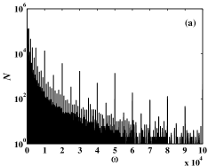
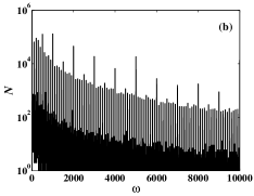
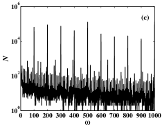
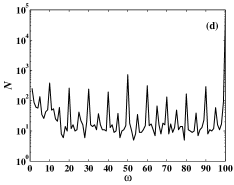
Due to a variety of diverse natural and human factors, the numbers' frequency of occurrence in human world shows an uneven behavior. With the help of search engines, Dorogovtsev et al found the occurrence frequencies of numbers in the World Wide Web pages are very different, 777 and 1000, for example, occur much more frequently than their neighbors Dorogovtsev-Mendes-Oliveira-2006-PA . This situation also happens in the stock market. The order price placement shows irrational preference of some numbers like 5, 10 or their multiples Gu-Chen-Zhou-2008c-PA in Chinese stock market. The first observation can trace back to Niederhoffer Niederhoffer-1965-OR in 1965, showing the price are often on integers, then on halves, on quarters, and Harris did more works on it Harris-1990-JFQA . Moreover, the frequency of first digit in stock's price or return does not correspond to the frequency of for each digit from 1 to 9 Pietronero-Tosatti-Tosatti-Vespignani-2000-PA ; Giles-2007-AEL , which also reflects people's number preference. Similar phenomenon exists in the number of trades, as shown in Fig. 2. This is accordant to the result of Alexander and Peterson Alexander-Peterson-2007-JFE . Fig. 2 plots the number of transactions with the same trade size as a function of the trade size for stock 000001 when the trade sizes are among 1 to shares. It is observed that there are several layers of spikes in these plots. Fig. 2(a) shows the first-layer spikes locating at and the second-layer spikes at , where . The third-layer spikes at and the fourth-layer spikes at can been seen in Fig. 2(b). Fig. 2(c) and (d) depict more layers of spikes for smaller trades. These spikes explain the jumps in the trade size PDFs in Fig. 1. Comparing Fig. 2(d) with other three plots, we find that the magnitude of for is much lower than those for large trades.
3.3 Fitting the distribution
We now fit the PDF of the normalized trade sizes of all the 22 stocks. The -Gamma distribution (Eq. (2)) is applied to model the PDF. For comparison, we also adopt the -exponential distribution Burr-1942-AMS ; Tsallis-1988-JSP ; Nadarajah-Kotz-2007-PA , student distribution Blattberg-Gonedes-1974-JB and log-normal distribution , which are defined as follows:
| (8) |
where and ,
| (9) |
where is the ``beta function'', location parameter , scale parameter and degrees of freedom parameter are positive, and
| (10) |
where and are corresponding mean and standard deviation respectively. The -exponential (Eq. (8)) has an asymptotic power-law tail whose tail exponent is
| (11) |
The empirical PDF and two fits ( and ) are illustrated in Fig. 3, because student and log-normal fits deviate considerably from the empirical PDF, especially the student function. It is visible that -exponential gives bad fit for small values, but a better fit than -Gamma for large values. Using taboo search and least-squares estimator, we obtain that the parameters of the -Gamma are , , and , while that of the -exponential are , and . According to Eq. (5) and Eq. (11), the tail exponents in the two models are 2.03 and 2.22, respectively.
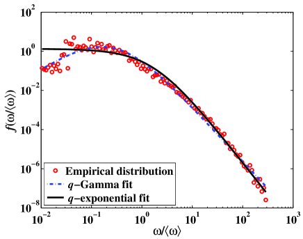
It is clear from Fig. 3 that the -Gamma distribution fits remarkably well the empirical PDF for the whole interval, while the -exponential does not. Here, the Cramér-von Mises criterion is used for judging the goodness-of-fit of the probability distribution compared to a given distribution Darling-1957-AMS , which is given by
| (12) |
where is the empirical cumulative distribution function, and is the corresponding theoretical distribution. In one-sample applications, the function can be described as follows Pearson-Stephens-1962-Bm ; Stephens-1970-JRSSB ,
| (13) |
where is the sample size. At the significance level 0.01, we find that for -Gamma is smaller than the critical value using Eq. 13, while the -exponential's is larger. So we can accept the hypothesis that the trade sizes data come from -Gamma distribution rather than -exponential distribution.
3.4 Determination of the tail exponent
Calibrating the -Gamma distribution already provides an estimate of the tail exponent. However, a careful comparison of the fitted curve with the empirical curve in the tail of Fig. 3 indicates that this estimate might be biased. Here, we utilize six methods to estimate the tail exponents, including the least-squares estimator (LSE) based on a linear fit of a power law, Hill's estimator (HE) that is a conditional maximum likelihood estimator Hill-1975-AS , Meerschaert and Scheffer's estimator (MSE) based on the behavior of moments Meerschaert-Schffer-1998-JSPI , Clauset, Shalizi and Newman's estimator (CSNE) based on maximum likelihood methods and the Kolmogorov-Smirnov statistic Clauset-Shalizi-Newman-2007-XXX , Fraga Alves's estimator (FAE) that is a location invariant Hill-type estimator Alves-2001-EX , and shift-optimized Hill estimator by Racz and Kertesz (RKE) that can handle data shifts Racz-Kertesz-2008-xxxx , which is an extension of the CSNE. The resultant estimates of the tail exponent using LSE, HE, MSE, CSNE, FAE and RKE are , , , , and , respectively. As pointed out by Racz et al., the MSE is unable to predict exponent above 2, and systematically underestimates the tail exponent Racz-Eisler-Kertesz-2008-XXX , while the FAE results in a high variance Racz-Kertesz-2008-xxxx .
4 Trading volume at different timescales
4.1 Bulk distribution
The distributions of trading volumes in different clock-time intervals have been studied for several other stock markets. The PDFs of the normalized trading volumes at different timescales are depicted in Fig. 4 for the Chinese stocks. The timescale ranges from 1 min to 240 min (1 trading day). The width of the PDF decreases with the increase of timescale. In addition, there is no scaling in these PDFs. For small values of , the density decreases with . For large values of , the PDFs decay in power-law forms.
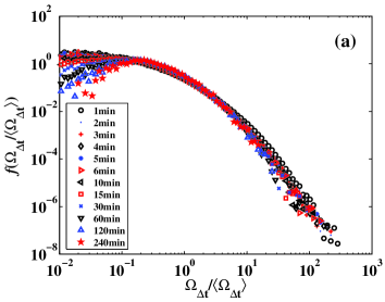
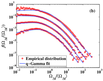
We also fitted these PDFs using -Gamma, -exponential and log-normal densities except the student density. Only the results of -Gamma fit for four typical cases with 1 min, 5 min, 15 min and 60 min are illustrated in Fig. 4(b). It is clear that the -Gamma functions fit remarkably the empirical PDFs, which is also reported for other markets with 1min, 2 min and 3 min Tsallis-Anteneodo-Borland-Osorio-2003-PA ; Queiros-2005-EPL ; deSouza-Moyano-Queiros-2006-EPJB ; Queiros-Moyano-deSouza-Tsallis-2007-EPJB . We use the Cramér-von Mises criterion again and find the values of for -Gamma function are smaller than the critical value at the significance level 0.01, when ranges from 1 min to 240 min.
| 1 min | 0.41 | 0.15 | 1.29 | 0.52 | 2.30 | |
|---|---|---|---|---|---|---|
| 2 min | 0.32 | 0.22 | 1.28 | 0.52 | 2.35 | |
| 3 min | 0.42 | 0.01 | 1.29 | 0.42 | 2.44 | |
| 4 min | 0.37 | 0.08 | 1.28 | 0.44 | 2.49 | |
| 5 min | 0.41 | 0.04 | 1.28 | 0.44 | 2.53 | |
| 6 min | 0.40 | 0.06 | 1.28 | 0.42 | 2.51 | |
| 10 min | 0.39 | 0.11 | 1.27 | 0.21 | 2.59 | |
| 15 min | 0.31 | 0.26 | 1.26 | 0.29 | 2.59 | |
| 30 min | 0.19 | 0.57 | 1.26 | 0.27 | 2.28 | |
| 60 min | 0.12 | 1.09 | 1.23 | 0.30 | 2.26 | |
| 120 min | 0.09 | 1.51 | 1.22 | 0.27 | 2.04 | |
| 240 min | 0.07 | 2.05 | 1.20 | 0.31 | 1.95 |
In contrast, the -exponential function and log-normal function have significant deviations from the empirical distributions, so we do not display them in Fig. 4(b). But -exponential grasps well the tail behaviors for small and log-normal grasps well for large values for large . This is not surprising since the -exponential (Eq.(8)) is a monotonically decreasing function and close to power law for large values while empirical PDFs show symmetrically for large values for large , tending to log-normal distribution. However, we cannot distinguish the -Gamma and -exponential functions in the tails. The estimated parameters using nonlinear least-squares regression for all the PDFs are listed in Table 1. All but one tail exponents are larger than two.
4.2 Tail exponents
In order to further confirm that the tail exponents of trading volumes at different timescales are consistently outside the Lévy regime, we also adopt the six different estimators used in Section 3 for the tail exponents. The results are presented in Table 2. For comparison, we also show the values obtained from the -Gamma fitting. For all the six tail exponent estimators, the value of trends up with the increase of . All the tail exponents obtained based on the MSE are less than two, while CSNE, LSE, FAE and RKE give tail exponents larger than two. For the Hill estimator, is less than two when and greater than two when . Again, we argue that the tail exponents of the trading volumes at different timescales do not belong to the Lévy regime.
| HE | MSE | CSNE | LSE | FAE | RKE | ||||
|---|---|---|---|---|---|---|---|---|---|
| 1 min | 2.30 | ||||||||
| 2 min | 2.35 | ||||||||
| 3 min | 2.44 | ||||||||
| 4 min | 2.49 | ||||||||
| 5 min | 2.53 | ||||||||
| 6 min | 2.51 | ||||||||
| 10 min | 2.59 | ||||||||
| 15 min | 2.59 | ||||||||
| 30 min | 2.28 | ||||||||
| 60 min | 2.26 | ||||||||
| 120 min | 2.04 | ||||||||
| 240 min | 1.95 |
5 Trading volume distribution for multiple trades
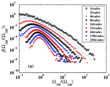
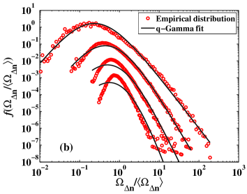
We now study the distributions of trading volumes for multiple transactions. The trading volumes are normalized by the averages for different . Fig. 5(a) illustrates the empirical PDFs for with . It is found that the PDFs have power-law tails. We use -Gamma functions to fit the PDFs, since the other distribution has significant deviations from the empirical distribution of . The estimated parameters for all the PDFs are listed in Table 3. Fig. 5(b) demonstrates the fits for four typical PDFs with . The -Gamma fits the data with good quality for small values of . For larger values of , the fits deviate considerably from the empirical data. Again, the Cramér-von-Mises tests is also used for judging the goodness-of-fit. The results are favorable only when at the significance level 0.01. The value of increases with the increase of when is larger than 8. So we can declare that the applicability of the -Gamma functions for multiple trades is restricted to the transaction number .
| 1 | 0.07 | 1.52 | 1.22 | 0.57 | 2.03 | |
| 2 | 0.04 | 2.68 | 1.17 | 0.47 | 2.20 | |
| 4 | 0.07 | 2.56 | 1.16 | 0.26 | 2.60 | |
| 8 | 0.07 | 3.28 | 1.14 | 0.29 | 2.86 | |
| 16 | 0.09 | 3.45 | 1.12 | 0.45 | 3.88 | |
| 32 | 0.09 | 3.37 | 1.12 | 0.65 | 3.96 | |
| 64 | 0.12 | 3.41 | 1.10 | 0.87 | 5.59 | |
| 128 | 0.11 | 3.39 | 1.10 | 0.92 | 5.61 | |
| 256 | 0.15 | 3.52 | 1.07 | 1.04 | 9.77 |
In order to determine the tail exponents, the six estimators mentioned in the previous sections are utilized. The resultant tail exponents are presented in Table 4. The values obtained from LSE, CSNE, FAE and RKE are greater than two, while those obtained from HE and MSE are less than two for small . There is an overall tendency that obtained from different method increases with . This can be considered as a significance of the central limit theorem meaning that for , the distribution converges to a Gaussian. The fact that the limit distribution is not a Lévy stable one is another indication that .
| HE | MSE | CSNE | LSE | FAE | RKE | ||||
|---|---|---|---|---|---|---|---|---|---|
| 1 | 2.03 | ||||||||
| 2 | 2.20 | ||||||||
| 4 | 2.60 | ||||||||
| 8 | 2.86 | ||||||||
| 16 | 3.88 | ||||||||
| 32 | 3.96 | ||||||||
| 64 | 5.59 | ||||||||
| 128 | 5.61 | ||||||||
| 256 | 9.77 |
6 Conclusion
The distributions of trade sizes and trading volumes are investigated based on the limit order book data of 22 liquid Chinese stocks listed on the Shenzhen Stock Exchange in the whole year 2003. The size distribution of trades for individual stocks exhibits jumps, which is caused by the fact that traders prefer to place orders with the size being certain numbers. The empirical PDFs of trading volumes at different timescales ranging from 1 min to 240 min can be modeled by the -Gamma functions. In contrast, the empirical PDFs of trading volumes for multiple trades can be fitted by the -Gamma functions only for small numbers of trades, . All the empirical PDFs exhibit power-law tails. In order to determine the tail exponents, we adopted six estimators (HE, MSE, LSE, CSNE, FAE and RKE). The estimated tail exponents using LSE, CSNE, FAE and RKE are greater than two, while those obtained from HE and MSE are less than two when or is small. Since HE and MSE may underestimate the tail exponents, we conclude that the tail exponents of trade sizes and trading volumes of Chinese stocks are well outside the Lévy regime.
Acknowledgements.
This work was partly supported by the National Natural Science Foundation of China (Nos. 70501011 and 70502007), the Fok Ying Tong Education Foundation (No. 101086), the Program for New Century Excellent Talents in University (No. NCET-07-0288), and the China Scholarship Council (No. 2008674017).References
- (1) J.M. Karpoff, J. Financ. Quart. Anal. 22, 109 (1987)
- (2) K. Chan, W.M. Fong, J. Financ. Econ. 57, 247 (2000)
- (3) F. Lillo, J.D. Farmer, R. Mantegna, Nature 421, 129 (2003)
- (4) M. Lim, R. Coggins, Quant. Financ. 5, 365 (2005)
- (5) R. Næs, J.A. Skjeltorp, J. Financ. Markets 9, 408 (2006)
- (6) W.X. Zhou (2007), http://arxiv.org/abs/0708.3198v2
- (7) X. Gabaix, P. Gopikrishnan, V. Plerou, H.E. Stanley, Nature 423, 267 (2003)
- (8) X. Gabaix, P. Gopikrishnan, V. Plerou, H.E. Stanley, Quart. J. Econ. 121, 461 (2006)
- (9) X. Gabaix, P. Gopikrishnan, V. Plerou, H.E. Stanley, J. Eur. Econ. Assoc. 4, 564 (2007)
- (10) X. Gabaix, P. Gopikrishnan, V. Plerou, H.E. Stanley, J. Econ. Dyn. Control 32, 303 (2008)
- (11) J.D. Farmer, L. Gillemot, F. Lillo, S. Mike, A. Sen, Quant. Financ. 4, 383 (2004)
- (12) P. Weber, B. Rosenow, Quant. Financ. 6, 7 (2006)
- (13) A. Joulin, A. Lefevre, D. Grunberg, J.P. Bouchaud (2008), http://arxiv.org/abs/0803.1769
- (14) P. Gopikrishnan, V. Plerou, X. Gabaix, H.E. Stanley, Phys. Rev. E 62, R4493 (2000)
- (15) V. Plerou, P. Gopikrishnan, X. Gabaix, L.A.N. Amaral, H.E. Stanley, Quant. Financ. 1, 262 (2001)
- (16) V. Plerou, P. Gopikrishnan, X. Gabaix, H.E. Stanley, Quant. Financ. 4, C11 (2004)
- (17) J.D. Farmer, F. Lillo, Quant. Financ. 4, C7 (2004)
- (18) S. Maslov, M. Mills, Physica A 299, 234 (2001)
- (19) V. Plerou, H.E. Stanley, Phys. Rev. E 76, 046109 (2007)
- (20) Z. Eisler, J. Kertész, Eur. Phys. J. B 51, 145 (2006)
- (21) Z. Eisler, J. Kertész, Physica A 382, 66 (2007)
- (22) E. Racz, Z. Eisler, J. Kertész (2008), arXiv:0803.3733
- (23) K.E. Lee, J.W. Lee, Physica A 383, 65 (2007)
- (24) C. Tsallis, C. Anteneodo, L. Borland, R. Osorio, Physica A 324, 89 (2003)
- (25) S.M.D. Queiros, Europhys. Lett. 71, 339 (2005)
- (26) J. de Souza, L.G. Moyano, S.M.D. Queiros, Eur. Phys. J. B 50, 165 (2006)
- (27) S.M.D. Queiros, L.G. Moyano, J. de Souza, C. Tsallis, Eur. Phys. J. B 55, 161 (2007)
- (28) S.N. Dorogovtsev, J.F.F. Mendes, J.G. Oliveira, Physica A 360, 548 (2006)
- (29) G.F. Gu, W. Chen, W.X. Zhou, Physica A 387, 5182 (2008)
- (30) V. Niederhoffer, Oper. Res. 13, 258 (1965)
- (31) L. Harris, J. Financ. Quart. Anal. 25, 291 (1990)
- (32) L. Pietronero, E. Tosatti, V. Tosatti, A. Vespignani, Physica A 293, 297 (2001)
- (33) D.E. Giles, Appl. Econ. Lett. 14, 157 (2007)
- (34) G.J. Alexander, M.A. Peterson, J. Financ. Econ. 84, 435 (2007)
- (35) I.W. Burr, Ann. Math. Stat. 13, 215 (1942)
- (36) C. Tsallis, J. Stat. Phys. 52, 479 (1988)
- (37) S. Nadarajah, S. Kotz, Physica A 377, 465 (2007)
- (38) R.C. Blattberg, N.J. Gonedes, J. Business 47(2), 244 (1974)
- (39) D.A. Darling, Ann. Math. Stat. 28, 823 (1957)
- (40) E.S. Pearson, M.A. Stephens, Biometrika 49, 397 (1962)
- (41) M.A. Stephens, J. Roy. Statist. Soc. B 32(1), 115 (1970)
- (42) B.M. Hill, Ann. Stat. 3, 1163 (1975)
- (43) M.M. Meerschaert, H.P. Scheffler, J. Stat. Plann. Inference 71, 19 (1998)
- (44) A. Clauset, C.R. Shalizi, M.E.J. Newman (2007), arXiv:0706.1062
- (45) M.I. Fraga Alves, Extremes 4, 199 (2001)
- (46) E. Racz, J. Kertesz (2008), in preparation