Non-commutativity as a measure of inequivalent quantization

Abstract

We show that the strength of non-commutativity could play a role in determining the boundary condition of a physical problem. As a toy model we consider the inverse square problem in non-commutative space. The scale invariance of the system is known to be explicitly broken by the scale of non-commutativity $\Theta$. The resulting problem in non-commutative space is analyzed. It is shown that despite the presence of higher singular potential coming from the leading term of the expansion of the potential to first order in $\Theta$, it can have a self-adjoint extensions. The boundary conditions are obtained, belong to a $1$-parameter family and related to the strength of non-commutativity.

Study of non-commutative spacetime michael ; calmet is a fascinating subject. The expectation that the spacetime could be non-commutative at small length scale has further accelerated the research work in this direction. Due to the non-commutativity of coordinates on a plane $(x,y)$ there exists an uncertainty relation

$$\Delta x\Delta y\sim\Theta\,,$$ (1)

where $\Theta$ is the non-commutativity parameter. Non-commutativity to a charged particle can arise due to the nontrivial nature of spacetime at small length scale or it may arise if the magnetic field, subjected perpendicular to the plane, is strong enough. However the idea of non-commutativity of spacetime is quite old way back in 1947 snyder , although that did not get much attention then. In quantum theory non-commutativity is a key object, for example coordinate $x$ and its conjugate $p$ are non-commutative,

$$\Delta x\Delta p\sim\hbar\,.$$ (2)

Even the generalized momenta $P_{i}$ in the magnetic field, $B$, background do not commute

$$\Delta P_{1}\Delta P_{2}\sim B\,.$$ (3)

The coordinates of a plane behave as canonical conjugate pairs and therefore do not commute in presence of a strong magnetic field perpendicular to the plane.

The strength of non-commutativity, $\Theta$, may have an intrinsic origin in spacetime or it may have origin in external magnetic field as stated before. However, the length scale, $\Theta$, introduced in the problem due to the non-commutativity can be exploited to heal the ultraviolet divergence of the problem under study. In a recent paper pulak we investigated the inverse square problem, $H=\bm{p}^{2}+\alpha\bm{r}^{-2}$, in non-commutative space in order to show how the length scale $\Theta$ can be successfully used to regularize the problem. Since the inverse square problem does not possess any dimensional parameter to start with it is a scale invariant problem. It can be understood from the transformation $\bf{r}\to\varepsilon\bf{r}$ and $t\to\varepsilon^{2}t$. The parameter $\varepsilon$ is the scaling factor. One can check that the classical action corresponding to the Hamiltonian $H$ is invariant under this transformation. See that the Hamiltonian $H$ transform as $H\to(1/\varepsilon^{2})H$. The Lagrangian $L$ associated with the system also transforms the same way, $L\to(1/\varepsilon)L$. It is now obvious that the action, $\mathcal{A}=\int dtL$, will be scale invariant under the transformation $\bf{r}\to\varepsilon\bf{r}$ and $t\to\varepsilon^{2}t$. In quantum mechanics, it has the following consequences. Let $\phi$ is an eigen-state of the Hamiltonian $H$ with eigenvalue $E$, i.e., $H\phi=E\phi$, then $\phi_{\varepsilon}=\phi(\varepsilon\bf r)$ will also be an eigen-state of the same $H$ but with energy, $E/\varepsilon^{2}$. The ground state therefore has no lower bound, implying that it does not have any bound state. It is however known from some physical problems, for example binding of electron in polar molecule giri3 , the near horizon states of a black hole govinda and other giri ; pulak1 ; pulak2 ; pulak3 that inverse square potential can bind particles. The theoretical interpretation of this binding can be obtained in terms of nontrivial quantization, which can be obtained by von Neumann method of self-adjoint extensions.

However once the inverse square problem is considered in a non-commutative plane, it looses its scale symmetry property due to the presence of dimensional parameter $\Theta$. To first order in the parameter, $\Theta$, the potential $V=\alpha/r^{2}$ in non-commutative plane becomes more singular, but then it belongs to an interesting class of interaction $V_{\mu}=\mbox{g}/r^{\mu}$, $\mu>2$ studied in mako . The interesting feature of the potential $V_{\mu}$ is that it possesses a localized state at the threshold of energy $E=0$. The states which has zero eigenvalue is usually considered as a transition point from bound states to scattering states. But due to the asymptotic nature of the potential of the type $V_{\mu}$ they can form bound states jamil , even at $E=0$. Apart from scale symmetry, inverse square problem has even larger symmetry, formed by three generators: the Hamiltonian $H$, the Dilatation generator $\mathcal{D}$ and the conformal generator $K$. It is called the $SO(2,1)$ algebra: $[\mathcal{D},H]=-i\hbar H$, $[\mathcal{D},K]=i\hbar K$, $[H,K]=2i\hbar\mathcal{D}$ wyb ; alfaro . We showed that with the introduction of non-commutativity the $so(2,1)$ symmetry of the system is broken explicitly and however in commutative limit the exact $so(2,1)$ symmetry is restored.

In the present article we extend our discussion of Ref. pulak further and find out a generic boundary condition for the zero energy localized state. The article is organized in the following fashion: First, we consider the inverse square interaction on a plane and discuss briefly how it changes when the co-ordinates of the plane become non-commutative. Second, we consider the non-commutative Hamiltonian obtained to first order in non-commutativity parameter $\Theta$. The possible bound sate spectrum is discussed in terms of generic boundary conditions. Finally, we conclude with some discussion.

We now consider a particle, interacting with the potential $V=\alpha/r^{2}$, on a non-commutative plane of the form

$$\left[\hat{x_{1}},\hat{x_{2}}\right]=2i\Theta,~{}\left[\hat{p_{1}},\hat{p_{2}}\right]=0,~{}\left[\hat{x_{i}},\hat{p_{j}}\right]=i\hbar\delta_{ij}\,.$$ (4)

However, the commutative limit $\Theta\to 0$ takes it to the standard algebra

$$\left[x_{1},x_{2}\right]=0,~{}\left[p_{1},p_{2}\right]=0,~{}\left[x_{i},p_{j}\right]=i\hbar\delta_{ij}\,.$$ (5)

It is useful to get a representation of the non-commutative coordinates $(\hat{x_{i}},\hat{p_{i}})$ in terms of the coordinates $(x_{i},p_{i})$. We choose a representation

$$\hat{x_{1}} = x_{1}-\Theta p_{2},~{}\hat{x_{2}}=x_{2}+\Theta p_{1}\,,$$

$$\hat{p_{1}} = p_{1},~{}\hat{p_{2}}=p_{2}\,,$$ (6)

for our purpose, but other representations are also possible. The Hamiltonian on non-commutative plane

$$H_{NC}={\hat{p_{1}}}^{2}+{\hat{p_{2}}}^{2}+\alpha/{\hat{r}}^{2}\,,$$ (7)

to first order in non-commutative parameter $\Theta$ can be written as

$$H_{NC}={p_{1}}^{2}+{p_{2}}^{2}+\alpha/{r}^{2}+2\alpha\Theta(x_{1}p_{2}-x_{2}p_{1})/r^{4}\,.$$ (8)

The presence of the potential $2\alpha\Theta(x_{1}p_{2}-x_{2}p_{1})/r^{4}$ breaks the scale invariance. We solved the eigenvalue problem

$$H_{NC}\psi_{NC}=E_{NC}\psi_{NC}\,,$$ (9)

for $E_{NC}=0$ and found a bound state with angular momentum $m$ for $\xi=\sqrt{\alpha+m^{2}}>1$ pulak . For large values of the non-commutative parameter, $\Theta$, it is also possible to get the expectation values of the Hamiltonian. Since the zero energy Schrödinger equation is exactly solvable it is possible to ask what is the most general boundary condition in this case. To be explicit, we consider an eigen-value problem of the form

$$\widehat{H_{NC}}\psi_{NC}\equiv-\frac{r^{4}}{\alpha m}\left(p_{1}^{2}+p_{2}^{2}+\alpha/r^{2}\right)\psi_{NC}=2\Theta\psi_{NC}\,,$$ (10)

Note that the dimensional parameter $2\Theta$ has been considered as the eigenvalue for our problem. All square-integrable solutions for different values of the parameter $\Theta$ correspond to the $E_{NC}=0$ degenerate states. Even for complex values of the parameter $\Theta$ if the solution $\psi_{NC}$ is square-integrable then it corresponds to the bound state with $E_{NC}=0$. Since our assumption in (4) is that the parameter $\Theta$ is real, we will restrict the parameter space to real line. It can be done if we can ensure that $\widehat{H_{NC}}$ is self-adjoint. From now onward the symmetric operator $\widehat{H_{NC}}$ will be investigated and a suitable boundary condition will be found out, which will make the operator self-adjoint.

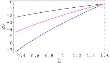
Figure 1: (color online) A plot of the non-commutativity parameter $2\Theta$ as a function of the self-adjoint extension parameter $\Sigma$ for $m=1$. It correspons to the equation (17). The blue curve corresponds to $\alpha=-1/10$, the pink curve corresponds to $\alpha=-1/6$ and the black curve corresponds to $\alpha=-1/3$.

Imposing a well defined boundary condition is important for getting a physical solution. We in this article we exploit von Neumann’s method to analyze $\widehat{H_{NC}}$. So, before actually making any symmetric extensions for the operator $\widehat{H_{NC}}$ a brief discussion about the von Neumann’s method is necessary here. Consider any symmetric operator, say, $\mathcal{B}$, which is for the moment taken to be unbounded. It is possible to define a domain $D(\mathcal{B})$ under which the operator $\mathcal{B}$ is symmetric. One can also obtain the adjoint operator, $\mathcal{B}^{*}$, corresponding to the operator $\mathcal{B}$. From the symmetric condition $\int_{0}^{\infty}\phi^{*}(r)\mathcal{B}\chi(r)dr=\int_{0}^{\infty}\left(\mathcal{B}^{*}\phi(r)\right)^{*}\chi(r)dr$, $\forall\chi(r)\in D(\mathcal{B})$ we can obtain the domain, $D(\mathcal{B}^{*})$. The operator $\mathcal{B}$ would be self-adjoint if the two domains are same, i.e., $D(\mathcal{B})=D(\mathcal{B}^{*})$. In terms of the deficiency indices $n_{\pm}$ reed one can have alternative definition of self-adjointness. The deficiency indices $n_{\pm}$ are the dimension of the kernel $Ker(i\pm\mathcal{B}^{*})$. If $n_{\pm}=0$, then the operator $\mathcal{B}$ is essentially self-adjoint. If $n_{+}=n_{-}=n\neq 0$, then $\mathcal{B}$ is not self-adjoint but admits self-adjoint extensions. Self-adjoint extensions can be characterized by $n^{2}$ parameters. Different values of the parameters give rise to different physics. For, $n_{+}\neq n_{-}$, the operator $\mathcal{B}$ does not have any self-adjoint extensions.

The operator, $\widehat{H_{NC}}$, we are analyzing in this work, acts on the functions defined over the Hilbert space of square-integrable functions with domain $\mathcal{L}^{2}[R^{+},rdr]$. Since the solution of the problem (10) has a similarity with the inverse square problem giri , $H\psi=E\psi$, it would be helpful to look at the short distance and asymptotic behavior of both the solutions. One can check that the solutions have an inverse relation to each other of the form

$$\lim_{r\to 0}\psi_{NC} \equiv \lim_{r\to\infty}\psi\,,$$

$$\lim_{r\to\infty}\psi_{NC} \equiv \lim_{r\to 0}\psi\,.$$ (11)

Due to this inverse behavior of the eigen-state we impose a nontrivial boundary condition for our problem at $r=\infty$. The operator $\widehat{H_{NC}}$ is essentially self-adjoint for $\xi^{2}\geq 1$ and has been discussed in pulak . Since any system is defined by a Hamiltonian and its corresponding domain, in our case $\widehat{H_{NC}}$ for $\xi^{2}\geq 1$ acts over the domain

$$\mathcal{D}_{0}=\{\psi\in\mathcal{L}^{2}(rdr),\psi(\infty)=\psi^{\prime}(\infty)=0\}\,.$$ (12)

Note the difference that the same condition (12) was imposed for the inverse-square problem giri but at $r\to 0$. Let us now investigate the operator for the interval $\xi\in(-1,1)$. In this region $\widehat{H_{NC}}$ is not essentially self-adjoint and therefore we need to make self-adjoint extensions of the original domain, so that the Hamiltonian becomes self-adjoint. We discuss the case $\xi\neq 0$ first, and then consider the case $\xi=0$ separately. The deficiency indices are $<1,1>$ for $\xi\in(-1,1)$. Since the number of deficiency space solutions are same for both types, there exist a self-adjoint extensions, characterized by a parameter, $\Sigma$. The domain under which $\widehat{H_{NC}}$ would be self-adjoint is given by

$$\mathcal{D}_{\Sigma}=\{\mathcal{D}_{0}+\psi_{+}+e^{i\Sigma}\psi_{-}\}\,.$$ (13)

The explicit form of the deficiency space solutions $\psi_{\pm}$ are given by

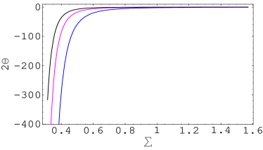
Figure 2: (color online) A plot of equation (19). Blue graph corresponds to $\alpha=-4$ and $m=2$. Pink graph corresponds to $\alpha=-9$ and $m=3$. Black graph corresponds to $\alpha=-16$ and $m=4$.

$$\psi_{+} = H_{\xi}\left(\frac{\sqrt{\alpha m}}{r}e^{-i\pi/4}\right)\,,$$ (14)

$$\psi_{-} = H_{\xi}\left(\frac{\sqrt{\alpha m}}{r}e^{+i\pi/4}\right)\,,$$ (15)

where $H_{\xi}$ is the modified Bessel function abr . The behavior of any function, belonging to the domain $\mathcal{D}_{\Sigma}$, near $r\to\infty$ can be found from the behavior of $\psi_{+}+e^{i\Sigma}\psi_{-}$ at asymptotic limit. Because the domain $\mathcal{D}_{0}$ goes to zero at $r\to\infty$, it does not contribute to the domain at $r\to\infty$. The asymptotic behavior of the domain is of the form

$$\lim_{r\to\infty}\left(\psi_{+}+e^{i\Sigma}\psi_{-}\right)\simeq\mathcal{A}_{+}\left(2r\right)^{-\xi}+\mathcal{A}_{-}\left(2r\right)^{\xi}\,,$$ (16)

where, $\mathcal{A}_{\pm}=-\frac{(\alpha m)^{\pm\xi/2}\pi i}{\sin(\pi\xi)}\frac{\cos(\frac{\Sigma}{2}\pm\frac{\pi\xi}{4})}{\Gamma(1\pm\xi)}$. The solution of (10) have to be matched with (16) to get the relation of the non-commutativity parameter $\Theta$ with the self-adjoint extension parameter $\Sigma$. We see that there is exactly one bound state with the non-commutativity, $2\Theta$, and eigenfunction, $\psi_{NC}$, being of the form

$$2\Theta = \frac{1}{\alpha m}\sqrt[\xi]{\frac{\cos\frac{1}{4}\left(2\Sigma+\xi\pi\right)}{\cos\frac{1}{4}\left(2\Sigma-\xi\pi\right)}}\,,$$ (17)

$$\psi_{NC} = \exp(im\phi)H_{\xi}\left(\frac{\sqrt{-2\Theta\alpha m}}{r}\right)\,.$$ (18)

In FIG. 1 the behavior of the parameter $2\Theta$ as a function of the self-adjoint extension parameter $\Sigma$ has been shown for three different values of the coupling constant $\alpha$ and for fixed value of the angular momentum quantum number $m$. Now let us come to the case for $\xi=0$, which can be handled similarly. The non-commutativity parameter corresponding to the bound state and the corresponding eigen-state are given by

$$2\Theta = \frac{1}{\alpha m}{\exp}\left(\frac{\pi}{2}{\cot}\frac{\Sigma}{2}\right)\,,$$ (19)

$$\psi_{NC} = \exp(im\phi)K_{0}\left(\frac{\sqrt{-2\Theta\alpha m}}{r}\right)\,.$$ (20)

respectively, where $K_{0}$ abr is the modified Bessel function. In FIG. 2 the parameter $2\Theta$ of (19) has been plotted as a function of the self-adjoint extension parameter $\Sigma$ for three sets of values of the pair $\alpha$ and $m$.

Finally, to first order in non-commutativity, $\Theta$, the inverse square problem has been discussed as a toy model to illustrate the connection of the boundary conditions with the strength of non-commutativity. The exact solvability of the $E_{NC}=0$ eigen-state has been exploited to get a generic boundary condition by making a suitable self-adjoint extensions for the problem. We treated the non-commutativity $\Theta$ as the eigen-value and obtained a generic boundary conditions under which the specra is restricted to the subspace of real axis.

References

- (1) M. R. Douglas and N. A. Nekrasov, Rev. Mod. Phys. 73, 977 (2001).
- (2) X. Calmet and M. Selvaggi, Phys. Rev. D74, 037901 (2006).
- (3) H. S. Snyder, Phys. Rev. 71, 38 (1947).
- (4) P. R. Giri, Phys. Lett. A372, 5123 (2008).
- (5) P. R. Giri, K. S. Gupta, S. Meljanac and A. Samsarov, Phys. Lett. A372, 2967 (2008).
- (6) T. R. Govindarajan, V. suneeta and S. Vaidya, Nucl. Phys. B583, 291 (2000).
- (7) P. R. Giri, Phys. Rev. A76, 012114 (2007).
- (8) P. R. Giri, Eur. Phys. J. C56, 147 (2008)
- (9) P. R. Giri, Int. J. Theor. Phys. 47, 1776 (2008).
- (10) P. R. Giri, Int. J. Theor. Phys. 47, 2583 (2008).
- (11) A. J. Makowski and K. J. Gorska, Phys. Lett. A362, 26 (2007).
- (12) J. Daboul and M. M. Nieto, Phys. Lett. A190, 357 (1994).
- (13) B. Wybourne, Classical Groups for Physics (Wiley, New York, 1974).
- (14) V. de Alfaro, S. Fubini and G. furlan, Nuovo Cimento 34A, 569 (1976).
- (15) M. Reed and B. Simon, Fourier Analysis, Self-Adjointness ( New York :Academic, 1975 )
- (16) M. Abromowitz, I. A. Stegun, Handbook of Mathematical Functions (Dover, New York, 1970).