Parallel hierarchical sampling: a practical multiple-chains sampler for Bayesian model selection

Abstract

This paper introduces the parallel hierarchical sampler (PHS), a Markov chain Monte Carlo algorithm using several chains simultaneously. The connections between PHS and the parallel tempering (PT) algorithm are illustrated, convergence of PHS joint transition kernel is proved and and its practical advantages are emphasized. We illustrate the inferences obtained using PHS, parallel tempering and the Metropolis-Hastings algorithm for three Bayesian model selection problems, namely Gaussian clustering, the selection of covariates for a linear regression model and the selection of the structure of a treed survival model.

Keywords: multiple-chains Markov chain Monte Carlo methods, Bayesian model selection, clustering, linear regression, classification and regression trees, survival analysis.

Introduction

Let $\theta\in\Theta$ be a random variable with distribution $\Pi(\theta)$. Markov chain Monte Carlo (MCMC) algorithms generate discrete-time Markov chains $\{\theta_{i}\}_{i=1}^{N}$ having $\Pi(\theta)$ as their unique stationary distribution (Robert and Casella (1999)). MCMC methods were pioneered by Metropolis and Ulam (1949) and by Metropolis et al. (1953) in the field of statistical mechanics. They have been adopted in statistics to approximate numerically expectations of the form $E_{\Pi}(g(\theta))$ where $g(\cdot)\in L^{2}(\Pi)$, i.e. the function $g(\cdot)$ is square integrable with respect to $\Pi(\theta)$. In Bayesian statistics, when the posterior distribution of a parameter $\theta$ given the data $X$, $\Pi(\theta\mid X)$, cannot be integrated analytically with respect to its dominating measure, its relevant features can be approximated via MCMC (Tierney (1994)). For a thorough analysis of the published MCMC algorithms, the reader may refer to Gelfand and Smith (1990), Smith and Roberts (1993), Neal (1993), Gilks et al. (1995), Gamerman (1997), Robert and Casella (1999) and Liu (2001) among others.

This paper illustrates a novel Markov chain algorithm, which we find useful for sampling from highly multimodal target distributions. We label this algorithm parallel hierarchical sampler (PHS) because of the prominent role of one chain with respect to the other generated chains. An important feature of PHS is that one array of Monte Carlo samples is generated using many chains run in parallel. PHS has in fact many connections with the Metropolis-coupled Markov chain Monte Carlo samplers of Swedensen and Wang (1987), Geyer (1991) and of Hukushima and Nemoto (1996). The main advantage of PHS with respect to other samplers is that the proposed updates are always accepted, thus ensuring optimal mixing of the resulting chain.

In Section $1$ of this paper we review some foundations of MCMC methods relevant for our work, with emphasis on the Metropolis-Hastings (MH) algorithm and on parallel tempering (PT). In Section $2$ we introduce the PHS algorithm, we prove the reversibility of its joint transition kernel with respect to its target distribution and we illustrate the relationships between PT and PHS. Sections $3$ and $4$ illustrate two examples comparing the inferences obtained using the PHS algorithm with those of MH and PT within the Bayesian model selection framework. The first example deals with data clustering. In the second example we consider the problem of selecting the best subset of covariates for a Gaussian linear regression model. Section $5$ illustrates the application of PHS for deriving posterior inferences for the structure of a treed survival model. Section $6$ discusses the current results and some ongoing developments of this work.

1 Foundations of MCMC algorithms

Let $\theta$ be a random variable with distribution $\Pi(\theta)$. In what follows, if f $\theta$ is continuous we let $f(\theta)$ be its probability density with respect to Lebesgue measure whereas if it is discrete $f(\theta)$ is its probability mass function. When it is not possible to obtain independent draws from $\Pi(\theta)$, Markov chains can be used to generate dependent realisations $\{\theta_{i}\}_{i=1}^{N}$ having stationary distribution $\Pi(\theta)$. Here the conditions under which such Markov chains can be constructed are stated and two algorithms are illustrated.

Let $K(\theta_{i},\theta_{i+1})$ be a transition kernel defining the probability to jump between any two values of $\theta$. If there exist an integer $d>0$ such that the probability of a transition between any two values $(\theta_{i},\theta_{i+1})$ with $f(\theta_{i})>0$ and $f(\theta_{i+1})>0$ in $d$ steps is positive, the transition kernel is $\Pi$-irreducible. $K(\theta_{i},\theta_{i+1})$ is aperiodic if it does not entail cycles of transitions among states. A sufficient condition for aperiodicity of an irreducible transition kernel is that $K(\theta_{i},\theta_{i})>0$ for some $\theta_{i}\in\Theta$. The transition kernel is reversible with respect to $\Pi(\theta)$ if it satisfies the detailed balance (DB) condition

$$f(\theta_{i})K(\theta_{i},\theta_{i+1})=f(\theta_{i+1})K(\theta_{i+1},\theta_{i}).$$ (1)

If a reversible and $\Pi$-irreducible transition kernel is also aperiodic, $\Pi(\theta)$ is its unique stationary distribution (Nummelin (1984), Robert and Casella (1999)). In such case, the strong law of large numbers holds for any function $g(\cdot)\in L^{2}(\Pi)$, that is

$$\lim_{N\to\infty}\left(\frac{1}{N}\sum_{i=1}^{N}g(\theta_{i})\right)=E_{\Pi}(g(\theta))\mbox{ a.s. }$$

Furthermore, under these conditions also the central limit theorem holds so that (Tierney (1994))

$$\sqrt{N}\left(\frac{1}{N}\sum_{i=1}^{N}g(\theta_{i})-E_{\Pi}(g(\theta))\right)\stackrel{{\scriptstyle d}}{{\rightarrow}}N(0,\sigma_{g,K}^{2}),$$

where the asymptotic standard deviation $\sigma_{g,K}$ depends on the function $g(\cdot)$ and on the transition kernel (Mira and Geyer (1999)).

1.1 The Metropolis-Hastings algorithm

The Metropolis-Hastings algorithm (Hastings (1970)) implements a family of transition kernels reversible with respect to an arbitrary target distribution $\Pi(\theta)$. Markov chains are generated by the MH algorithm by converting the independent draws from a proposal distribution $q(\cdot)$ into dependent samples from $\Pi(\theta)$ through a simple accept/reject mechanism (Chib and Greenberg (1995), Billera and Diaconics (2001)). Without loss of generality, in what follows we let $q(\cdot)$ assign zero probability to the current state $\theta_{i}$. Under this condition, the MH transition kernel can be written as

$$K_{MH}(\theta_{i},\theta_{i+1})=\alpha_{MH}(\theta_{i},\theta_{i+1})q(\theta_{i+1}\mid\theta_{i})\text{ if }\theta_{i+1}\neq\theta_{i},$$ (2)

where the acceptance ratio $\alpha_{MH}(\theta_{i},\theta_{i+1})$ is defined as

$$\alpha_{MH}(\theta_{i},\theta_{i+1})=1\wedge\frac{f(\theta_{i+1})q(\theta_{i}\mid\theta_{i+1})}{f(\theta_{i})q(\theta_{i+1}\mid\theta_{i})}.$$ (3)

The irreducibility and aperiodicity of the MH transition kernel and its practical performance for specific sampling problems hinge mainly on the appropriate choice of the proposal distribution $q(\cdot)$ (Tierney (1994)). Reversibility with respect to $f(\theta)$ can be immediately verified by checking that $(1)$ holds using equations $(2)$ and $(3)$. Furthermore, by equation $(3)$ the MH algorithm requires the evaluation of the function $f(\theta)$ only up to a multiplicative constant, which is a key feature for Bayesian applications where the target posterior distribution is typically known up to a finite multiplicative factor (Gelfand and Smith (1990)).

1.2 Parallel tempering

Parallel tempering (PT) is a multiple-chains extension of the MH algorithm which can improve mixing when the MH sample paths exhibit high correlations (Geyer (1991)). Poor mixing of the MH algorithm typically arises when the target distribution is multimodal. As emphasized by Swedensen and Wang (1987), Hukushima and Nemoto (1996) and Liu (2001), in statistical mechanics such distributions may arise in the analysis of stochastic interacting particle systems, such as spin glasses and the Ising model. In Bayesian statistics multimodality of the posterior distribution might occur when an informative prior disagrees with the likelihood, in highly structured hierarchical models and when several nuisance parameters are integrated out of the joint posterior. An impotant example of the latter case is provided by Bayesian model selection methods using the marginal posterior probability of the model structure.

The PT algorithm appears in the literature in different forms and under different labels. Swedensen and Wang (1987) introduced the “Replica Monte Carlo” algorithm, Geyer (1991) labeled his algorithm “Metropolis-coupled MCMC”, whereas the algorithm of Hukushima and Nemoto (1996) is labeled “Exchange Monte Carlo”. Here we give a unified description of PT encompassing those of Geyer, Liu and Hukushima and Nemoto.

Let $1=T_{1}\leq T_{2}\leq...\leq T_{M}<\infty$ be a fixed real-valued vector of temperature levels. For each value of the index $m\in[1,M]$ a heated version of the target density $f(\theta)$ is defined by “powering up” $f(\theta)$ as

$$f_{m}(\theta)=\frac{f(\theta)^{\frac{1}{T_{m}}}}{C_{m}},$$ (4)

where $C_{m}>0$ is a finite normalising constant depending on the temperature parameter $T_{m}$. The latter acts as a smoother of the target distribution of the cold chain, which has temperature one, so that the heated densities have fatter tails and less pronounced modes with respect to $f_{1}(\theta)$. The PT sampler proceeds, at each iteration, by alternating an update step with a swap step. The former is carried out by updating each chain independently of the others typically via the Gibbs sampler using one or more embedded MH steps. To perform the swap step, let $s_{i}$ have value $0$ if update is chosen at iteration $i$ and $1$ if swap is chosen instead. The proposal probability $q^{{}^{\prime}}_{s}(s_{i}\mid s_{i-1})$ describes how the two steps are combined by the sampler. Geyer (1991) adopts the deterministic proposal $q^{{}^{\prime}}_{s}(s_{i}\mid s_{i-1})=1_{\{s_{i-1}=0\}}$, whereas Liu (2001) defines an independent PT sampler using $q^{{}^{\prime}}_{s}(s_{i}\mid s_{i-1})=s$ where $s\in(0,1)$ is a fixed swap proposal rate. Let the indexes $j_{i}$ and $k_{i}$ range over $(1,...,M)$ and let $\theta_{i}^{j_{i}}$ indicate the state of chain $j_{i}$ at iteration $i$. The second proposal employed by the PT sampler, $q^{{}^{\prime\prime}}_{s}(\theta_{i}^{j_{i}},\theta_{i}^{k_{i}})$ defines the probability that at iteration $i$ a swap is attempted between the current values of the chains with indexes $(j_{i},k_{i})$. In Geyer (1991), in Hukushima and Nemoto (1996) and in Liu (2001) this proposal is taken as independent of the current states of the two chains $\theta_{i}^{j_{i}},\theta_{i}^{k_{i}}$ but only dependent on thei indexes $(j_{i},k_{i})$. Specifically, the swap proposal used by these authors is uniform over all possible values of the ordered couple $(j_{i},k_{i})$ with $k_{i}\neq j_{i}$ and a swap is accepted with probability

$$\alpha_{s}([\theta_{i}^{j_{i}},\theta_{i}^{k_{i}}],[\theta_{i}^{k_{i}},\theta_{i}^{j_{i}}])=1\wedge\frac{f_{j_{i}}(\theta_{i}^{k_{i}})f_{k_{i}}(\theta_{i}^{j_{i}})}{f_{j_{i}}(\theta_{i}^{j_{i}})f_{k_{i}}(\theta_{i}^{k_{i}})},$$ (5)

ensuring the reversibility of the PT sampler with respect to its joint target distribution. When the independent updates of each chain are carried out using a single MH step, the joint transition kernel of the PT sampler is

$$K_{PT}(\theta_{M,i},\theta_{M,i+1})=(1-q^{{}^{\prime}}_{s}(s_{i}\mid s_{i-1}))\prod_{w=1}^{M}q(\theta^{w}_{i+1}\mid\theta^{w}_{i})\alpha_{MH}(\theta^{w}_{i},\theta^{w}_{i+1})+$$

$$+q^{{}^{\prime}}_{s}(s_{i}\mid s_{i-1})\sum_{j_{1}=1}^{M}\sum_{\stackrel{{\scriptstyle k_{i}=1}}{{k_{i}\neq j_{i}}}}^{M}q^{{}^{\prime\prime}}_{s}(j_{i},k_{i})\alpha_{s}([\theta_{i}^{j_{i}},\theta_{i}^{k_{i}}],[\theta_{i}^{k_{i}},\theta_{i}^{j_{i}}]).$$ (6)

where $\theta_{M,i}=[\theta_{i}^{1},...,\theta_{i}^{M}]$ is the state of all $M$ chains at iteration $i$. From $(6)$ it can be seen that when the within-chain updates produce high correlations, PT increases mixing for all chains through their successful swaps. Analogously to the MH algorithm, the irreducibility and aperiodicity of the PT transition kernel depend mainly on the proposal distribution for the within-chains update, $q(\cdot)$ and on that of the cross-chains swaps $q^{{}^{\prime\prime}}_{s}(\cdot)$. A proof of the reversibility of the PT algorithm can be found in Hukushima and Nemoto (1996). Finally we note that, analogously to the MH algorithm, by equations $(4)$ and $(5)$ the implementation of PT does not require knowledge of the finite normalising constants $\{C_{m}\}_{m=1}^{M}$ so that it is a suitable MCMC sampler for Bayesian posterior simulation.

2 The parallel hierarchical sampler

A key difficulty affecting the general applicability of the PT sampler is its dependence on the values of the temperatures $\{T_{m}\}_{m=1}^{M}$. In statistical mechanics, the latter are chosen with reference to the physical properties of the systems being modeled, such as the energy barriers implied by successive temperature levels. However, in statistics the equilibrium distributions being simulated seldom possess analogous interpretations. An alternative solution illustrated in this Section is to employ a multiple chains sampler such that the equilibrium distributions of all chains is the same but the proposal distribution used to update each chain is different. Specifically, definition $1$ describes a multiple-chains sampler which does not employ temperatures and combines independent updates with swap moves within each iteration.

Definition 1

Let a multiple-chains MCMC sampler proceed by carrying out both the following two steps at each iteration:

• let the index $m_{i}$ be drawn from a discrete proposal distribution $q^{{}^{\prime\prime}}_{s}(m_{i}\mid m_{i-1})$ symmetric with respect to its arguments;

• swap the current value of chain $m_{i}$ and that of the first chain;

• update independently the remaining $M-2$ chains each having the same marginal target distribution $f(\theta)$.

At point $ii)$ above, we indicate as $q^{{}^{\prime\prime}}_{s}(\cdot)$ the swap proposal to emphasize the analogy with the PT algorithm. We label the algorithm defined above parallel hierarchical sampler (PHS) because the first chain is given a prominent role and the update of all chains is carried out in parallel analogously to PT. To provide a simple proof of the reversibility of the PHS joint kernel, in this Section we assume that the chains $(2,..M)$ are updated using a single MH step and that the transition kernels for these MH updates satisfy the conditions illustrated in Tierney (1994) so that they are irreducible and aperiodic with respect to their marginal target distributions. In addition, we assume that the symmetric proposal distribution $q^{{}^{\prime\prime}}_{s}(\cdot)$ allows for swaps between the first chain and any of the other chains. Under these conditions the marginal transition kernel for the first chain of the PHS algorithm is irreducible and aperiodic with respect to its target distribution. Let $\theta_{M}=\theta\times\theta\times...\times\theta$ be the $M$-fold cartesian product of the random variable $\theta$. By the arguments of Section $1$, if the PHS joint transition kernel is also reversible with respect to the product density $\mu(\theta_{M})$ having all marginals equal to $f(\theta)$, then $\mu(\theta_{M})$ is the unique joint stationary distribution of the sampler. The reversibility of the PHS is proved in the following theorem.

Theorem 1

The joint transition kernel of the PHS algorithm of Definition $1$ is reversible with respect to the joint distribution having product density or probability mass function $\mu(\theta_{M})$.

• The DB condition for the PHS algorithm is

  $$\frac{\mu(\theta_{M,i})}{\mu(\theta_{M,i+1})}=\frac{K_{PHS}(\theta_{M,i+1},\theta_{M,i})}{K_{PHS}(\theta_{M,i},\theta_{M,i+1})},$$ (7)

  where $K_{PHS}(\theta_{M,i+1},\theta_{M,i})$ is the PHS joint transition kernel. When the independent updates of the chains $(2,...,M)$ are carried out via a MH step, the PHS joint transition kernel can be written explicitely as

  $$K_{PHS}(\theta_{M,i},\theta_{M,i+1})=\sum_{m_{i}=2}^{M}q^{{}^{\prime\prime}}_{s}(m_{i}\mid m_{i-1})\prod_{\stackrel{{\scriptstyle j=2}}{{j\neq m_{i}}}}^{M}q(\theta^{j}_{i+1}\mid\theta^{j}_{i})\alpha_{MH}(\theta_{i}^{j},\theta_{i+1}^{j}).$$ (8)

  Each summand in $(8)$ is the product of the marginal transition kernel for the swap transition and those of the $(M-2)$ independent MH updates for the remaining chains. The former coincides with the proposal $q^{{}^{\prime\prime}}_{s}(m_{i}\mid m_{i-1})$ because the PHS swap acceptance ratio is equal to one. This fact will be motivated in the next Section by illustrating the relationship between PHS and PT. Under $(8)$ the DB condition $(7)$ can be rewritten as

  $$\sum_{m_{i}=2}^{M}q^{{}^{\prime\prime}}_{s}(m_{i}\mid m_{i-1})\prod_{\stackrel{{\scriptstyle j=2}}{{j\neq m_{i}}}}^{M}q(\theta^{j}_{i+1}\mid\theta^{j}_{i})\alpha_{MH}(\theta_{i}^{j},\theta_{i+1}^{j})=$$

  $$=\sum_{m_{i}=2}^{M}q^{{}^{\prime\prime}}_{s}(m_{i-1}\mid m_{i})\prod_{\stackrel{{\scriptstyle j=2}}{{j\neq m_{i-1}}}}^{M}q(\theta^{j}_{i}\mid\theta^{j}_{i+1})\alpha_{MH}(\theta_{i+1}^{j},\theta_{i}^{j})$$ (9)

  For any given value of $m_{i}$, by the reversibility of $(2)$ and $(3)$ with respect to $f(\theta)$, the $M-2$ MH transition probabilities on the left-hand side of $(9)$ are equal to their corresponding terms on the right-hand side. By taking $q^{{}^{\prime\prime}}_{s}(\cdot)$ symmetric with respect to $m_{i}$ and $m_{i-1}$, for all values of $m_{i}$ each summand on the left-hand side of $(9)$ equals its corresponding term on the right-hand side, so that the equality $(9)$ holds.           $\diamond$

Equation $(8)$ implies that, as for the MH and PT algorithms, PHS does not require knowledge of the normalising constant of its marginal target distributions $C$ so that it is suitable for sampling from target distributions known only up to a finite multiplicative factor.

2.1 Relationship between PHS and parallel tempering

Both $(6)$ and $(8)$ are mixtures of marginal transition kernels respectively defining the joint transition probabilities for the PT and PHS algorithms. The analogy between the two is that $(M-1)$ out of the $M$ parallel chains are auxilliary and Monte Carlo estimates are computed using the samples of the first chain only. There are two important differences between the two samplers. At each iteration, the PHS transition kernel mixes over the update and swap steps as described in Definition $1$ whereas in PT they are alternated according to the proposal probability $q^{{}^{\prime}}_{s}(s_{i}\mid s_{i-1})$. Since the former step typically generates local transitions whereas the latter produces larger jumps, PT creates unnecessary competition between local and global mixing. Furthermore, in PHS all marginal target distributions are not powered up using a temperature coefficient as in PT. The rationales to avoid the temperature coefficients are both conceptual and practical. From a Bayesian prespective, the main conceptual issue is that the temperatures do not appear neither in the likelihood function nor in the prior, so that it is not clear whether they should be treated analogously to the other parameters indexing the target posterior distribution. In practice, determining sensible values for the temperatures requires a lenghty trial-and-error process in the pursuit of a target swap rate between pairs of chains. Moreover, since the normalising constants of the marginal posterior distributions depend on their temperatures, updating of the latter is not possible unless for conjugate families. The simulated tempering algorithm of Geyer and Thompson (1995) implements a single chain sampler for both the parameter $\theta$ and a single temperature coefficient $T$. The latter is treated as a discrete random variable and its update is carried out using a data dependent pseudo-prior in order to simplify the normalising constant of the joint posterior distribution from the Metropolis-Hastings acceptance ratio. An interesting point in simulated tempering is that the temperature is not constrained to be larger than one, so that when $T$ is close to zero the posterior distribution becomes concentrated around its modes. However, although practically useful, the simulated tempering algorithm does not clarify the nature of the temperature parameter and it does not explain how the posterior normalising constant could be seen as part of a prior distribution for the same parameter.

In PHS, since all temperatures have value $1$, the Metropolis swap acceptance ratio $(5)$ is equal to one, so that the proposed moves for the first chain are always accepted. This property marks the most evident difference between the sample paths of the first chain of PHS, those of the cold chain of PT and those of the MH algorithm.

2.2 PHS as a variable augmentation scheme

Variable augmentation for MCMC samplers was first introduced by Tanner and Wong (1987). Its general principle is that convergence of one of the generated chains can be sped up by cleverly augmenting the state-space using additional coefficients. Conditionally on these auxilliary variables the posterior distribution of the parameters of interest can typically be sampled exactly. The PHS algorithm can be seen as a variable augmentation scheme where the additional coefficients are $M-1$ replicates of the parameter of interest itself. In PHS the target distribution of the first chain does not depend on the other replicates. At each iteration, the $M-1$ auxilliary chains having index $(2,..,M)$ directly provide a set of potential updates for the chain of interest.

2.3 PHS and multiple-try Metropolis algorithms

Liu et al. (2000) illustrate a generalization of the single chain Metropolis algorithm where multiple values from the same proposal distribution are drawn at each iteration of the sampler. To attain detailed balance, a generalized Metropolis acceptance ratio involving several pseudo-current chain states is computed. This multiple-try generalized Metropolis sampler actually mimics the behaviour of a multiple chains algorithm using the sme proposal within each of the generated chains. Therefore, the main analogy between the algorithm of Liu et al. (2000) and PHS is that many candidates are available at each iteration to update one chain of interest. In Liu et al. (2000), only one of such updates is retained and the Metropolis ratio is modified accordingly. In PHS, all such values not used for swapping with the first chain are retained and individually updated. Moreover, the proposal mechanism generating all potential updates is not constrained to be the same for all chains.

3 An illustrative example: MCMC generation of mixtures of Gaussian variates

In this Section we report a comparison between the empirical performance of MH and PHS algorithms for generating a sample from a mixture of scalar Gaussian random variables. We use the results of one simulation to illustrate the typical difference between the performance of the two samplers.

Within the MH algorithm we use a random walk uniform proposal distribution on the interval $(\theta_{i}-\delta,\theta_{i}+\delta)$, where $\theta_{i}$ is the current value of the chain. We construct a PHS algorithm using the same Metropolis updates within chains $(2,...,M)$ and by adopting a uniform swap proposal distribution $q^{{}^{\prime\prime}}(m_{i}\mid m_{i-1})=\frac{1}{M-1}$. For this example we let $M=10$, that is we employ nine auxilliary chains having the same proposal spread $\delta=1$ as that of the MH sampler. The PHS sampler was run for one hundred thousand iterations. In order to make the computational cost for both samplers comparable, the MH algorithm was run for one million iterations. All chains were started at the same initial value equal to zero.

The number of components of the mixture was set to $5$, their means were generated uniformly at random over the interval $(-10,10)$ obtaining the values $(-8.85,-2.65,2.63,3.85,4.35)$. Their standard deviations were generated uniformly at random over the interval $(0.1,1)$, obtaining the values $(0.18,0.51,0.50,0.42,0.24)$. Finally, the unnormalised weights of the mixture components were drawn uniformly at random over the interval $(1,5)$. Thier normalised values are $(0.22,0.22,0.23,0.15,0.18)$. Figure $1$ shows the probability density of the mixture over the range $(-13.5,6.6)$. The mixture components having means $(2.63,3.85)$ and standard deviations $(0.50,0.42)$ are very close and they do not result in two separate modes of the mixture density. Figure $2$ compares the histograms of the MH draws with that of the first PHS chain. The former sampler effectively located the three closest modes to its starting value whereas PHS successfully visited all four modes of its target distribution.

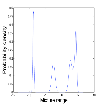
Figure 1: the Gaussian mixture density used as target distribution for the Metropolis sampler and for the parallel hierarchical sampler. The distribution is a mixture of five Gaussian components having means $(-8.85,-2.65,2.63,3.85,4.35)$, standard deviations $(0.18,0.51,0.50,0.42,0.24)$ and weights $(0.22,0.22,0.23,0.15,0.18)$.

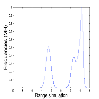
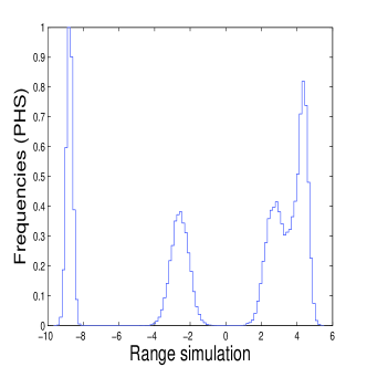
Figure 2: the plot on the left-hand side shows the histogram of the Metropolis draws. On the right-hand side, the plot represent the histogram of the draws of the first PHS chain. Thanks to the swapping mechanism, the latter successfully visited all the four modes of its marginal target distribution whereas the Metropolis algorithm only visited the three closes models to its starting value.

4 Application to the selection of covariates for the Bayesian linear regression model

The covariates selection problem for the Bayesian Gaussian linear regression has been addressed model using MCMC methods by Mitchell and Beauchamp (1988), Smith and Kohn (1996), George and McCulloch (1993), Carlin and Chib (1995), George and McCulloch (1997), Raftery et al. (1997), Kuo and Mallick (1998), Dellaportas et al. (2002) and Clyde and George (2004) among many others.

Using the same notation as in George and McCulloch (1997), we let the distribution of the $n$-dimensional random vector $Y$ be multivariate Gaussian with mean $X_{\gamma}\beta_{\gamma}$ and covariance matrix $\sigma^{2}I_{n}$, being $(\sigma,\beta,\gamma)$ a priori unknown. The $p$-dimensional model index $\gamma$ has elements $\gamma_{j}$ taking value one if the $j$th covariate is used for the computation of the mean of $Y$ and zero otherwise. Here $\beta_{\gamma}$ and $X_{\gamma}$ include respectively the elements of the $p$-dimensional column vector $\beta$ associated to non-zero components of $\gamma$ and the corresponding columns of $X$. The latter is a real-valued $n\times p$ matrix representing $p$ potential predictors for the mean of $Y$. Within this framework, the variable selection problem consists of deriving inferences for $\gamma$ conditionally on the data $(Y,X)$. In order to compute such inferences, we employ MH, PT and PHS to generate draws from the marginal posterior probability of the model index,

$$P(\gamma\mid Y,X)\propto P(\gamma)P(Y\mid\gamma,X).$$

In this Section we adopt the same form of the marginal posterior probability of $\gamma$ as in Nott and Green (2004), letting

$$P(\gamma\mid Y,X)\propto(1+n)^{-\frac{S(\gamma)}{2}}\left(Y^{{}^{\prime}}Y-\frac{n}{n+1}Y^{{}^{\prime}}X_{\gamma}(X^{{}^{\prime}}_{\gamma}X_{\gamma})^{-1}X^{{}^{\prime}}_{\gamma}Y\right)^{-\frac{n}{2}}$$ (10)

We also note that if the predictors included in $X_{\gamma}$ tend to be collinear, the matrix $X^{{}^{\prime}}_{\gamma}X_{\gamma}$ can be almost singular and the right hand side of equation $(11)$ may be numerically unstable. In such instances, we find that computing the marginal posterior using the Cholesky decomposition of $X^{{}^{\prime}}_{\gamma}X_{\gamma}$, as in Smith and Kohn (1996), yields numerically stable results.

In order to compare the PHS estimates with that of the MH and of the PT algorithms, we consider two simulated datasets. In both cases the dependent data is $Y\sim N(X_{\gamma}\beta_{\gamma},6.25I_{180})$ and the regression coefficients are set at $\beta_{\gamma_{j}}=2j/15$ for $j=1,...,15$. For the first dataset, $X$ is generated as a $180\times 15$ matrix of i.i.d. draws from a Normal distribution with mean zero and variance $1$. Let $Z_{1},...,Z_{16}$ be $i.i.d$ Gaussian column vectors of length $180$ with mean zero and covariance matrix $I_{180}$. For the second dataset a strong collinearity was induced among the predictors $X$ by letting

$$X_{j} = Z_{j}+2Z_{16}\mbox{ for }j=1,...,15,$$

where $X_{j}$ is the $j$th column of $X$, as in Section $5.2.1$ of George and McCulloch (1997). Here we will compare the estimation results of the MH algorithm with those of the cold chain of PT and of PHS for the two datasets using the estimated marginal posterior inclusion probabilities for each predictor and their Monte Carlo standard errors (MCSEs). The former are defined as $\bar{\gamma_{j}}=\sum_{i=1}^{N}\gamma^{i}_{j}/N$ where $i=1,...,N$ is the iteration index and $\gamma^{i}_{j}$ is the $i$th draw for the $j$th predictor. As illustrated by Geweke (1992), Nott and Green (2004) and by George and McCulloch (1997), the MCSE for the inclusion probability of the $j$th predictor is

$$MCSE(\bar{\gamma}_{j})=\sqrt{\frac{1}{N}\sum_{|h|<N}\left(1-\frac{|h|}{N}\right)A_{j}(h)},$$

where $A_{j}(h)$ is the lag $h$ autocovariance of the chain of realisations for $\gamma_{j}$. For ergodic Markov chains, as $N\rightarrow\infty$ the MCSE converges, up to an additive constant independent of the transition kernel, to the MCMC standard error $\sigma_{g,K}$ (Mira and Geyer (1999)) where $g(\gamma_{j})=E(\gamma_{j}\mid Y,X)$ for this example.

Three independent batches of chains were run for fifty thousand iterations. For PT and PHS, we used nine chains which target distributions are defined as in $(4)$ with cold distribution $(11)$. For PT, the heated chains were defined using the same array of equally spaced temperatures with range $1-5$. For each sampler, the starting values of $\gamma$ for all chains was the null model. All within-chain updates were carried out using a component-wise random scan Metropolis algorithm proposing a change of the current value of each parameter $\gamma_{j}$ at every iteration, as in Denison et al. (1998). The cross-chains proposals $q_{s}(\cdot)$ and $q^{{}^{\prime\prime}}_{s}(\cdot)$ were taken uniform. Since the PT algorithm also depends on the proposal $q^{{}^{\prime}}_{s}(\cdot)$, we run three batches of PT chains using Liu’s proposal $q^{{}^{\prime}}_{s}(s_{i}\mid s_{i-1})=s$ with $s=0.2,0.5,0.8$.

Figure $5$ illustrates the simulation results. The plots on the top row refer to the data without collinearity whereas the plots on the bottom report the inferences for the data with collinearity. By comparing the two rows of Figure $5$, it appears that the induced collinearity among the predictors did not affect the estimation results for any of the samplers. The estimated inclusion probabilities are generally increasing with respect to the true value of their regression parameters $\beta_{\gamma}$ for all samplers and for both datasets, with a noticeable shift occurring between the fifth and the sixth predictors (which regression parameters are respectively $\beta_{\gamma_{5}}=0.67$ and $\beta_{\gamma_{6}}=0.8$). Higher swap rates for the PT algorithm, marked by circles and by plus signs in Figure $5$, result in a large decrease in the estimated inclusion probabilities for the predictors corresponding to large regression coefficients $\beta_{\gamma}$. The estimated inclusion probabilities for the predictors associated to low values of the regression coefficients are the lowest for the MH algorithm whereas the PHS estimates are the highest for these predictors. Finally, the plots on the right-hand side of Figure $5$ suggest that for this example the precision of the three samplers, as measured by their MCSEs, is roughly comparable.

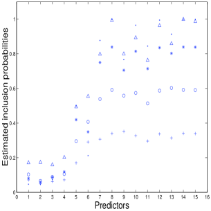
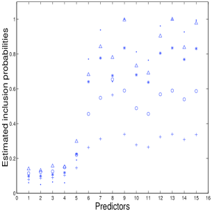
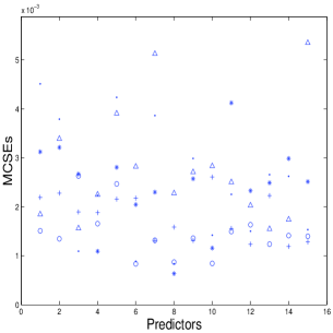
Figure 3: estimated marginal posterior inclusion probabilities for the fifteen predictors (left) and their Markov chain standard errors (right). The plots on top refer to the simulated data without collinearity and the bottom plots refer to the data with collinearity. In all plots, plus signs correspond to the results of the PT algorithm with $s=0.8$, circles correspond to PT with $s=0.5$ and asterisks mark the PT results with $s=0.2$. Triangles identify the results of the PHS algorithm and dots mark those of MH. The PHS estimates for the marginal inclusion probabilities are the highest for the predictors associated to low values of their regression coefficients $\beta_{\gamma}$, whereas high swap rates for the PT algorithm produce wrong estimates of the inclusion probabilities for the predictors associated to high values of $\beta_{\gamma}$. The precision of the three algorithms, as measured by their MCSEs, appears to be comparable.

5 Application to the estimation of the structure of a survival CART model

In regression and classification trees (CART) the sample is clustered in disjoint sets called leaves. The leaves are the final nodes of a single-rooted binary partition of the covariates space which we will refer to as the tree structure. Within each leaf, the response variable is modeled according to the regression, or classification or with the survival analysis frameworks (Breiman et al. (1984)). Bayesian CART models appeared in the literature with the papers of Chipman et al. (1998) and Denison et al. (1998). The MCMC model search algorithms developed in these two papers treat the tree structure as an unknown parameter and explore its marginal posterior distribution using the Gibbs sampler and the MH algorithm. In this example we focus on tree models for randomly right-censored survival data (Gordon and Olshen (1995), Davis and Anderson (1989), M.Leblanch and J.Crowley (1992a), M.Leblanch and J.Crowley (1992b)). The first Bayesian survival tree model has been proposed by Pittman et al. (2004), who adopted a Weibull leaf sampling density and a step-wise greedy model search algorithm based on the evaluation of all the possible splits within each node. The main strength of this model is that it incorporates a flexible parametric form for the survival function and that the tree search quickly converges to a mode in the model space. In this Section, we propose a fully Bayesian analysis of the marginal posterior distribution over the space of tree structures using PHS under the Weibull leaf likelihood. Upon convergence, besides providing the structure of the estimated modal tree, the realisations of the cold chain provide a sample from the marginal posterior distribution of the tree structure which can be employed to rank the combinations of the covariates defining the visited trees as a function of their estimated marginal posterior inclusion probabilities.

5.1 Tree structure marginal posterior distribution

Let the survival times $\{t_{j}\}_{j=1}^{n}$ be independent random variables conditionally on the tree structure $(b,\zeta)$ and on the Weibull leaf parameters $(\alpha_{\zeta},\beta_{\zeta})$. Under this assumption, the joint sampling density of the survival times can be written as

$$f(t\mid X,\delta,b,\zeta,\alpha_{\zeta},\beta_{\zeta})=\prod_{k=1}^{b}\prod_{j=1}^{n}\left(\left(\alpha_{k}\beta_{k}t_{j}^{\alpha_{k}-1}\right)^{\delta_{j}}e^{-\beta_{k}t_{j}^{\alpha_{k}}}\right)^{1_{k,j}},$$ (11)

where $b$ is the number of leaves, $\delta_{j}$ takes value $1$ for exact observations and $0$ for right censored observations and $1_{k,j}=1_{\{X_{j}\in\zeta_{k}\}}$ is $1$ if the covariate profile of the $j$th sample unit is included in $\zeta_{k}$, which is the subset of the covariate space corresponding to leaf $k=1,...,b$, and $0$ otherwise. Under a discrete uniform prior for the tree structure, the marginal posterior probability $P(b,\zeta\mid t,X,\delta)$ can be obtained, up to a multiplicative constant, by integrating $(11)$ with respect to the conditional prior distribution for the array of leaf parameters $(\alpha_{\zeta},\beta_{\zeta})$. In this work we place independent uninformative priors for each Weibull leaf parameter. Sun (1997) provides an accurate study of different uninformative priors for the Weibull distribution. In particular, Sun’s paper indicates that $h_{k}(\alpha_{k},\beta_{k})=1/\alpha_{k}\beta_{k}$ is the Jeffreys’ prior and the first order matching prior for the Weibull parameters of leaf $k$ given the parametrization $(11)$. Sun also shows that, under $h_{k}(\alpha_{k},\beta_{k})$, the joint posterior density for the leaf parameters $(\alpha_{k},\beta_{k})$ is proper when the number of data points is larger than one and if all the observations falling in leaf $k$ are not equal. For this specification of the prior structure, the joint posterior of the tree structure and of the leaf parameters can be written as

$$f(b,\zeta,\alpha_{\zeta},\beta_{\zeta}\mid t,X,\delta)\propto\prod_{k=1}^{b}\frac{1}{\alpha_{k}\beta_{k}}\prod_{j=1}^{n}\left(\left(\alpha_{k}\beta_{k}t_{j}^{\alpha_{k}-1}\right)^{\delta_{j}}e^{-\beta_{k}t_{j}^{\alpha_{k}}}\right)^{1_{k,j}}.$$ (12)

The Weibull scale parameters $\beta_{k}$ can be integrated out of the joint posterior $(12)$ analytically. The resulting integrated posterior density is

$$f(b,\zeta,\alpha_{\zeta}\mid t,X,\delta)\propto\prod_{k}\frac{\Gamma(\sum_{j}\delta_{j}1_{k,j})\alpha_{k}^{\sum_{j}\delta_{j}1_{k,j}-1}e^{(\alpha_{k}-1)\sum_{j}\delta_{j}\log(t_{j})1_{k,j}}}{(\sum_{j}t_{j}^{\alpha_{k}}1_{k,j})^{\sum_{j}\delta_{j}1_{k,j}}}.$$ (13)

Under $(13)$, analytical integration of the Weibull index parameters $\alpha_{k}$ is not possible. For any given model, the Monte Carlo method of Chib and Jeliazkov (2001) can be employed to compute a simulation-based approximation of the marginal posterior probability of the tree structure. However, since this integration needs to be performed for each visited tree, the computational cost of Chib and Jeliazkov’s method makes it unsuitable for any iterative model search. In this work we approximate the tree structure marginal posterior probability using the Laplace expansion of equation $(13)$, which can be written as

$$P(b,\zeta\mid t,X,\delta)\approx exp\left(b\frac{\log(2\pi)}{2}+\sum_{k=1}^{b}\left(\log(l(\hat{\eta}_{k}))-\frac{\log(-l_{2}(\eta_{k}))|_{\hat{\eta}_{k}}}{2}\right)\right),$$ (14)

where $\hat{\eta}_{k}$ is the posterior mode of the Weibull leaf log index parameter $\eta_{k}=\log(\alpha_{k})$. The derivation of equation $(14)$ and the explicit forms of the functions $l(\eta)$ and $l_{2}(\eta)$ are reported in the Appendix.

5.2 Marginal posterior inference for the tree structure

In the CART framework, as in the clustering problem illustrated in Section $3$, the main challenge for constructing efficient within-chain proposal distributions is the lack of a distance metric between different models. This issue has been also noted by Brooks et al. (2003) in the context of the reversible jump MCMC algorithm (Green (1995)). Our specification of the within-chain proposal distribution generalizes the approaches of Denison et al. (1998) and Chipman et al. (1998) by devising two additional within-chain transitions besides their insert, delete and change moves. For the within-chain updates we propose a transition at random among the following five types:

• Insert: sample a leaf at random and insert a new split by randomly selecting a new splitting rule.

• Delete: sample at random a leaf pair with common parent and at most one child split and delete it.

• Change: resample at random one splitting rule.

• Permute: sample a random number of splits and permute at random their splitting rules.

• Graft: sample at random one of the tree branches and graft it to one of the leaves of a different branch.

Chipman et al. (1998) noted that their MCMC algorithm can effectively resample the splitting rules of nodes close to the tree leaves but the rules defining splits close to the tree root are seldom replaced. In our specification of the within-chain transitions, move number $4$ aims at improving sampling of the splitting rules at all levels of the tree structure. Furthermore, the fifth move type allows the sampler to jump to a tree structure distinct from the current one without changing its splitting rules.

Having adopted a multiple-chains algorithm, we also devised two types of cross-chains transitions. The first is the cross-chains version of the insert, graft and change transitions, swapping the elements of the tree structure required to perform corresponding pairs of transitions across chains. The second class of cross-chains transitions includes a whole tree swap between chains.

At iteration $i$, the PHS algorithm for this example proceeds as follows:

• choose at random one of the heated chains $m_{i}\in[2,M]$ and propose at random one of the cross-chains moves, accepting the swap with probability $1$.

• update each of the remaining $M-2$ chains independently using the five types of within-chain transitions and the MH acceptance probability.

5.3 Analysis of a set of cancer survival times

Colorectal adenocarcinoma ranks second as a cause of death due to cancer in the western world and liver metastasis is the main cause of death in patients with colorectal cancer (Pasetto et al. (2003)). The survival times of $622$ patients with liver metastases from a colorectal primary tumor were collected along with their clinical profiles by the International Association Against Cancer (http://www.uicc.org). Table $1$ reports a description of the nine available clinical covariates. The survival times of this dataset are currently included in the R library locfit (http://www.locfit.info). This data has been analyzed by Hermanek and Gall (1990) using non-parametric methods, by Antoniadis et al. (1999) using their wavelet-based method for estimating the survival density and the instantaneous hazard function and by Kottas (2003), who employed a Dirichlet process mixture of Weibull distributions to derive a Bayesian non-parametric estimate of the survival density and of the hazard function. Haupt and Mansmann (1995) employed this dataset to illustrate the non-parametric tree fitting techniques for survival data implemented in the S-plus function survcart. The aim of this Section is showing that the estimates of $(b,\zeta)$ obtained using the PHS algorithm and the approximate marginal posterior $(14)$ provide meaningful inferences for the prognostic significance of the available covariates. For each covariate, the latter will be represented by its estimated posterior inclusion probability, i.e. by the proportion of sampled models which structure depends on the covariate.

	Name	Symbol	Description
$1$	Diam. largest LM	DLM	$(1,20)$mm
$2$	Age	AGE	$(18,88)$years
$3$	Diagnosis of LM	TD	synchrone/metachron with CPT
$4$	Gender	SEX	M = $55.8\%$, F = $44.2\%$
$5$	Lobar involvement	LI	unilobar/bilobar
$6$	Number of LM	NLM	$(1,20+)$
$7$	Locoregional disease	LRD	yes/no
$8$	Metastatic stage	TNM	local/regional/distant
$9$	Location PT	LOC	colon/rectum

Table 1: description of the covariates for the liver dataset. The data include several types of clinical covariates, such as continuous (DLM), discrete (AGE, NLM) and categorical (all others).

A PHS using twenty parallel chains was run for fifty thousand iterations, the starting tree for each chain being the root model. Consistently with the PHS algorithm described in Section $5.2$, for this analysis we used a uniform swap proposal distribution $q_{s}(\cdot)$. On the top row, Figure $6$ shows the unnormalised log posterior tree probability for the models visited by the cold chain, plotted respectively versus the iteration index and versus their number of leaves. The posterior sampling for the cold chain moved quickly towards areas of high marginal posterior probability models, which leaf range is $10-14$, the best tree having $12$ leaves. The bottom plot of Figure $6$ shows the estimated marginal posterior inclusion probabilities for all the covariates. According to these estimates, the covariates with maximal prognostic significance are the diameter of the largest liver metastasis and the number of liver metastases, followed by their locoregional disease status, the patients’age at diagnosis, the localisation of their primary tumor and their lobar involvement status. The estimated inclusion probabilities of the remaining covariates suggest that, for this sample, their values do not discriminate among significantly different survival clusters.

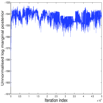
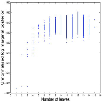
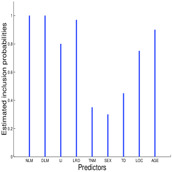
Figure 4: the top plots show the unnormalised log marginal posterior probability of the tree structure for the models visited along the PHS posterior simulation by the cold chain. The horizontal axis in the left plot represents the iteration index, whereas in the right plot it represents the number of leaves of the corresponding tree. The plot on the bottom shows the estimated marginal posterior inclusion probabilities for the nine covariates. Those with maximal prognostic significance are the diameter of the largest liver metastasis, the number of liver metastases, the locoregional disease status, the patients’age at diagnosis, the localisation of their primary tumor and their lobar involvement status.

Figure $7$ shows the structure of the estimated modal posterior tree. The depth of the leaves in this figure reflects the number of splits required to generate them. For any given tree structure $(b,\zeta)$, posterior inferences for $(\alpha_{\zeta},\beta_{\zeta})$ can be obtained by further simulation using their full conditional posterior distributions, which can be easily derived from the full conditional posterior $(12)$. In order to maintain the focus of this Section on the application of PHS for tree selection, here we adopt the Kaplan-Meier (KM) survival curves as non-parametric estimates of the survival probabilities within each leaf. Table $2$ reports the number of patients clustered within each leaf of the modal tree and the values of their KM survival probabilities at $12$, $24$ and $36$ months. The bold figures in Table $2$ correspond respectively to the highest and to the lowest estimated survival probabilities at the three time points. The lowest survival correspond to leaves number $1$ and $2$ for all the three time points. These two groups are defined by high values of the first two covariates in the tree, which are the diameter of the largest liver metastasis and the number of liver metastases. The highest estimated survival probabilities at $12$, $24$ and $36$ months correspond to leaf number $8$ which is characterised by at most one liver metastasis of small diameter, local spreading of the cancer and no locoregional disease.

Leaf Number	Cluster size	$\hat{P}_{km}(t\geq 12)$	$\hat{P}_{km}(t\geq 24)$	$\hat{P}_{km}(t\geq 36)$
$1$	$63$	$0.70$	$0.23$	$\mathbf{0.03}$
$2$	$148$	$\mathbf{0.58}$	$\mathbf{0.14}$	$\mathbf{0.04}$
$3$	$34$	$0.75$	$0.53$	$0.43$
$4$	$78$	$0.85$	$0.50$	$0.28$
$5$	$42$	$0.85$	$0.50$	$0.16$
$6$	$48$	$0.80$	$0.57$	$0.26$
$7$	$31$	$0.90$	$0.81$	$0.64$
$8$	$42$	$\mathbf{1.00}$	$\mathbf{0.84}$	$\mathbf{0.77}$
$9$	$30$	$0.69$	$0.25$	$0.19$
$10$	$32$	$0.65$	$0.30$	$0.10$
$11$	$42$	$0.68$	$0.59$	$0.29$
$12$	$31$	$0.97$	$0.76$	$0.29$

Table 2: number of observations falling in each leaf of the estimated posterior modal tree and Kaplan-Meier survival probabilities at $12$, $24$ and $36$ months. The highest survival probabilities correspond to leaf number $8$, which is defined by a low number of local metastases of small diameter and by the absence of locoregional disease. The lowest survival probabilities correspond to leaves $1$ and $2$, which are characterized respectively by metastases of large diameter and by a large number of smaller metastases.

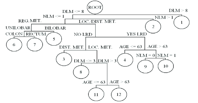
Figure 5: tree structure of the estimated modal tree found by the PHS simulation. The lowest estimated survival probabilities at $1$, $2$ and $3$ years correspond to leaves number $1$ and $2$, which are defined by high values of the two key covariates (NLM,DLM), whereas the best estimated survival corresponds to leaf number $8$, which is defined by the non-linear interaction of (DLM,NLM,LRD and LOC).

6 Discussion

This paper presents a novel multiple chains algorithm for Markov chain Monte Carlo inference, which we labeled parallel hierarchical sampler. We emphasized the main terms of comparison to evaluate the parallel hierarchical sampler, that are the Metropolis algorithm, the muliple-try Metropolis algorithm of Liu et al. (2000) and parallel tempering. Whilst in the Metropolis sampler high acceptance rates usually produce high autocorrelations and slow convergence (Roberts et al. (1997b)), by construction PHS produces a chain which always moves but which exhibits low serial dependence. As it can be seen be comparing the PT and PHS joint transition kernels, reported by equations $(6)$ and $(8)$, the first advantage of PHS with respect to PT is that its swap proposal has a simpler form. This is because in PHS both types of transitions are performed at each iterations instead of being sampled according to the distribution $q_{s}^{{}^{\prime}}(s_{i}\mid s_{i-1})$. The second practical advantage of PHS with respect to PT is that its implementation does not require choosing a set of temperature values. When little is known about the equilibrium distribution being studied, we regard this feature of PHS as a potentially major advantage. Furthermore, although the algorithm presented in Section $2$ allows for a different proposal distribution within each of the chains indexed $m=2,...,M$, this is not even a necessary requirements for the implementation of PHS.

As pointed out by Geyer (1991), the attractive feature of multiple-chains MCMC samplers such as PT and PHS is that their target distribution factors into the product of the marginal distributions for each chain despite the fact that these chains are made dependent by the swap transitions. Under the conditions of Section $2$ we prove in Theorem $1$ that the samples generated by the PHS algorithm converge weakly to such product distribution.

In Section $2$ we also noted that the complexity of multiple-chains transition kernels, which for PT and PHS are mixtures of their marginal transition kernels, largely prevents a direct analytical comparison of their convergence properties. Direct comparison of the transition kernels $(6)$ and $(8)$ leads to major analytical difficulties and so far it has not been possible to establish an ordering between the two kernels using the criteria illustrated in Peskun (1973), Meyn and Tweedie (1994) and Mira (2001). Although it falls beyond the scope of this paper, we regard the development of computable ordering criteria for mixtures of Markov chain transition kernels as a key area which deserves further investigation.

Following Huelsenbeck et al. (2001), the last three Sections of this paper emphasise the relevance of multiple-chains MCMC algorithms for estimating the posterior model probabilities in a variety of settings. In Sections $3$ and $4$ we provide two examples comparing numerically the inferences obtained by the Metropolis-Hastings algorithm with those of PT and PHS. In these two Sections we focussed on comparing the posterior inferences without considering the computational time required to produce them. The rationale behind this choice is that the computational time required by multiple-chains samplers is highly dependent on the available computational resources. For instance, if all chains used by PT and PHS are run in parallel on several processors, their run time may be comparable to that of the single-chain Metropolis-Hastings sampler, whereas if all chains are updated sequentially using one processor their run time is, of course, much longer.

In Section $3$ we observed that for the Gaussian clustering the PHS algorithm appears to explore the space of cluster configurations more effectively with respect to MH and PT using the same within-chain proposal mechanism for all samplers. For the example of Section $4$ we observed that using high swap proposal rates for the PT sampler leads to wrong estimates of the marginal posterior inclusion probabilities with and without collinearity among the predictors $X$. However, by measuring the precision of the three MCMC algorithms by their Markov chain standard errors we did not find a significant advantage of the multiple-chains samplers with respect to the MH algorithm.

Section $5$ illustrates the application of PHS for deriving inferences for the structure of a treed survival model. One of the main differences between of Sections $4$ and $5$ is that the focus of the former is the selection of the relevant main regression effects whereas in the latter the key elements defining different survival groups are the non-linear interactions among the predictors defining the tree structure. The top-right plot in Figure $6$ shows that the approximated marginal posterior probability of the tree structure under the Weibull model does not increase monotonically with the number of leaves. Under the Weibull model we used the Laplace expansion to approximate the tree structure marginal posterior probability. The Schwarz approximation (Schwarz (1978)) was also considered. The penalty term of the Schwarz approximation increases with the model dimension, thus it represents a cost for complexity factor. However, given a fixed number of leaves this approximation favours trees allocating the data more unevenly across leaves. Therefore, employing the Schwarz approximation when many covariates are available might result in assigning significant posterior probability to large and unbalanced trees, leading to overfitting small groups of survival data. On the other hand, the penalty associated to the Laplace approximation has a complex form involving the tree size, the log Weibull parameters $\eta_{i}$ and the survival times along with their censoring indicators. Evaluation of this approximation for a variety of tree structures showed that this penalty is strictly increasing with the tree dimension but it does not favour unbalanced trees. Using the Laplace expansion to approximate the model’s marginal posterior probability and the PHS algorithm to sample from it, we find meaningful posterior inferences for a set of colorectal cancer survival data. The estimated modal tree separates the short-term survivors, who are characterised by a large number of liver metastases of large size, from the long-term survivors, who present a few local metastases of small size without further symptoms.

Finally, in Sections $3$, $4$ and $5$ we addressed qualitatively the issue of convergence of the chains produced by the three MCMC algorithms by considering their acceptance rates and the fluctuations of their marginal posterior probabilities. Being the model spaces inherently non-metric, it was not possible to use the state-dependent criteria commonly used to assess the convergence of Markov chains to their stationary distributions illustrated in Carlin and Cowles (1996), Roberts et al. (1997a) or in Robert (1998) among others. Although it is beyond the scope of this paper, in light of the increasing relevance of model selection problems we consider the development of appropriate convergence measures an important field for future research.

Appendix

The Laplace approximation is the second order Taylor expansion of the logarithm of the integrated posterior $(14)$ around its posterior mode. In order to derive the approximation, it is convenient to parametrize equation $(14)$ as a function of $\eta_{k}=\log(\alpha_{k})$, so that the variables to be integrated out have support on the real line. Under this parametrization, stable estimates of the posterior modes $\{\hat{\eta}_{k}\}_{k=1}^{b}$ can be computed numerically. For each leaf the log integrated conditional posterior is

$$l(\eta_{k}) \propto \log(\Gamma(\sum_{j}\delta_{j}1_{k,j}))+(\eta_{k}-1)\sum_{j}\delta_{j}1_{k,j}+e^{\eta_{k}}\sum_{j}\delta_{j}\log(t_{j})1_{k,j}$$

$$- \sum_{j}\delta_{j}1_{k,j}\log(\sum_{j}t_{j}^{e^{\eta_{k}}}1_{k,j}).$$

The penalty arising from the Laplace approximation is proportional to minus the logarithm of the second derivative of the log integrated posterior taken with respect to the leaf parameters $\{\eta_{k}\}$. The second derivative of the function $l(\eta_{k})$ is

$$l_{2}(\eta_{k})=e^{\eta_{k}}\left(\sum_{j}\delta_{j}\log(t_{j})1_{k,j}-\frac{\sum_{j}\delta_{j}1_{k,j}\sum_{j}t_{j}^{e^{\eta_{k}}}(\log(t_{j}))^{2}1_{k,j}}{\sum_{j}t_{j}^{e^{\eta_{k}}}1_{k,j}}\right).$$

Summing the approximation over the $b$ leaves yields the right-hand side of equation $(15)$.

References

- Antoniadis et al. (1999) A. Antoniadis, G. Grégoire, and G. Nason. Density and hazard rate estimation for right-censored data by using wavelet methods. Journal of the Royal Statistical Society, series B, 61:63–84, 1999.
- Billera and Diaconics (2001) L.J. Billera and P. Diaconics. A geometric interpretation of the Metropolis-Hastings algorithm. Statistical Science, 16:335–339, 2001.
- Breiman et al. (1984) L. Breiman, J.H. Friedman, R.A. Olshen, and C.J. Stone. Classification and Regression Trees. Chapman and Hall, New York, 1984.
- Brooks et al. (2003) S.P. Brooks, P. Giudici, and G.O. Roberts. Efficient construction of Reversible Jump MCMC proposal distributions. Journal of the Royal Statistical Society, series B, 65:3–55, 2003.
- Carlin and Chib (1995) B.P. Carlin and S. Chib. Bayesian model choice via Markov chain Monte Carlo methods. Journal of the Royal Statistical Society, series B, 57, 1995.
- Carlin and Cowles (1996) B.P. Carlin and M.K. Cowles. Markov chain Monte Carlo convergence diagnostics: A comparative review. Journal of the American Statistical Association, 91:883–904, 1996.
- Chib and Greenberg (1995) S. Chib and E. Greenberg. Understanding the Metropolis-Hastings algorithm. The American Statistician, 49:327–335, 1995.
- Chib and Jeliazkov (2001) S. Chib and I. Jeliazkov. Marginal likelihood from the Metropolis-Hastings output. Journal of the American Statistical Society, 96:270–281, 2001.
- Chipman et al. (1998) Hugh A. Chipman, Edward I. George, and Robert E. McCulloch. Bayesian CART model search. Journal of the American Statistical Society, 93:935–947, 1998.
- Clyde and George (2004) M. Clyde and E.I. George. Model Uncertainty. Statistical Science, 19:81–94, 2004.
- Davis and Anderson (1989) R.B. Davis and J.R. Anderson. Exponential survival trees. Statistics in Medicine, 8, 1989.
- Dellaportas et al. (2002) P. Dellaportas, J.J. Forster, and I. Ntzoufras. On Bayesian model and variable selection using MCMC. Statistics and Computing, 12:27–36, 2002.
- Denison et al. (1998) D.G.T. Denison, B.K. Mallick, and A.F.M. Smith. A Bayesian CART algorithm. Biometrika, 85, 1998.
- Gamerman (1997) D. Gamerman. Markov chain Monte Carlo: Stochastic Simulation for Bayesian Inference. Chapman and Hall, 1997.
- Gelfand and Smith (1990) A.E. Gelfand and A. F. M. Smith. Sampling-based approaches to calculating marginal densities. Journal of the American Statistical Society, 85:398–409, 1990.
- George and McCulloch (1997) E.I. George and R.E. McCulloch. Approaches for Bayesian variable selection. Statistica Sinica, 7:339–373, 1997.
- George and McCulloch (1993) E.I. George and R.E. McCulloch. Variable selection via Gibbs sampling. Journal of the American Statistical Association, 88:882–889, 1993.
- Geweke (1992) J. Geweke. Evaluating the accuracy of sampling-based approaches to the calculation of posterior moments. In: Bayesian Statistics 4, J.M. Bernardo, J.O. Berger, A.P. Dawid and A.F.M. Smith editors; Oxford Press, pages 169–194, 1992.
- Geyer and Thompson (1995) C. J. Geyer and E.A. Thompson. Annealing Markov Chain Monte Carlo with applications to ancestral inference. Journal of the American Statistical Association, 90:909–920, 1995.
- Geyer (1991) C.J. Geyer. Markov chain Monte Carlo maximum likelihood. Computing Science and Statistics: Proceedings on the 23rd Symposium on the Interface, New York, 1991.
- Gilks et al. (1995) W.R. Gilks, S. Richardson, and D. J. Spiegelhalter. Markov chain Monte Carlo in practice. Chapman and Hall, 1995.
- Gordon and Olshen (1995) L. Gordon and R.A. Olshen. Tree-structured survival analysis. Cancer Treatment Reports, 69, 1995.
- Green (1995) P.H. Green. Reversible Jump Markov chain Monte Carlo computation and Bayesian model determination. Biometrika, 82:711–732, 1995.
- Hastings (1970) W.K. Hastings. Monte Carlo sampling methods using Markov chains and their applications. Biometrika, 57-1:97–109, 1970.
- Haupt and Mansmann (1995) G. Haupt and U. Mansmann. Survival trees in Splus. Advances in Statistical Software 5, pages 615–622, 1995.
- Hermanek and Gall (1990) P. Hermanek and F.P. Gall. Uicc Studie zur Klassifikation von Lebermetastasen. Chirurgie der Lebermetastasen und primaren malignen Tumoren, 1990.
- Huelsenbeck et al. (2001) J.P. Huelsenbeck, F. Ronquist, R. Nielsen, and J.P. Bollback. Bayesian inference of Phylogeny and its impact on evolutionary biology. Science, 14:2310–2314, 2001.
- Hukushima and Nemoto (1996) K. Hukushima and K. Nemoto. Exchange Monte Carlo method and application to Spin Glass simulations. Journal of the Physical Society of Japan, 65:1604–1620, 1996.
- Kottas (2003) A. Kottas. Nonparametric Bayesian survival analysis using mixtures of Weibull distributions. To appear in the Journal of Statistical Planning and Inference, 2003.
- Kuo and Mallick (1998) L. Kuo and B. Mallick. Variable selection for regression models. Sankhya, B, 60:65–81, 1998.
- Liu (2001) J.S. Liu. Monte Carlo Strategies in Scientific computing. Springer, 2001.
- Liu et al. (2000) J.S. Liu, F. Liang, and W.H. Wong. The multiple-try method and local optimization in Metropolis sampling. ournal of the American Statistical Association, 95:121–134, 2000.
- Metropolis and Ulam (1949) N. Metropolis and S. Ulam. The Monte Carlo method. Journal of the American Statistical Association, 44:335–341, 1949.
- Metropolis et al. (1953) N. Metropolis, A. Rosenbluth, M. Rosenbluth, M. Teller, and E. Teller. Equations of state calculations by fast computing machines. J. Chem. Phys., 21:1087–2092, 1953.
- Meyn and Tweedie (1994) S. Meyn and R.L. Tweedie. State-dependent criteria for convergence of Markov chains. The Annals of Applied Probability, 4:149–168, 1994.
- Mira (2001) A. Mira. Ordering and improving the performance of Monte Carlo Markov chains. Statistical Science, 16:340–350, 2001.
- Mira and Geyer (1999) A. Mira and C. Geyer. Ordering Monte Carlo Markov chains. Technical Report 632, School of Statistics, University of Minnesota, 1999.
- Mitchell and Beauchamp (1988) T.J. Mitchell and J.J. Beauchamp. Bayesian variable selection in linear regression. Journal of the American Statistical Association, 83:1023–1032, 1988.
- M.Leblanch and J.Crowley (1992a) M.Leblanch and J.Crowley. Relative risk trees for censored survival data. Biometrics, 48, 1992a.
- M.Leblanch and J.Crowley (1992b) M.Leblanch and J.Crowley. Survival trees by goodness of split. Journal of the American Statistical Association, 88, 1992b.
- Neal (1993) R.M. Neal. Probabilistic inference using Markov chain Monte Carlo methods. Technical report, Department of Computer Science, University of Toronto, 1993.
- Nott and Green (2004) D.J. Nott and P.J. Green. Bayesian veriable selection and the Swendsen-Wang algorithm. Journal of Computational and Graphical Statistics, 13:141–157, 2004.
- Nummelin (1984) E. Nummelin. General Irreducible Markov Chains on Non-Negative Operators. Cambridge University Press, 1984.
- Pasetto et al. (2003) L.M. Pasetto, Rossi E., and Monfardini S. Liver metastases of colorectal cancer: medical treatment. Anticancer, 23:4245–56, 2003.
- Peskun (1973) P.H. Peskun. Optimum Monte Carlo sampling using Markov chain. Biometrika, 60:607–612, 1973.
- Pittman et al. (2004) J. Pittman, E. Huang, H. Dressman, C.F. Horng, S.H. Cheng, M.H. Tsou, C.M. Chen, A. Bild, E.S. Iversen, A.T. Huang, J.R. Nevins, and M. West. Integrated modeling of clinical and gene expression information for personalized prediction of disease outcomes. Proceedings of the National Academy of Sciences, 101:8431–8436, 2004.
- Raftery et al. (1997) A. E. Raftery, D. Madigan, and J. A. Hoeting. Bayesian model averaging for linear regression models. Journal of the American Statistical Society, 92:179–191, 1997.
- Robert (1998) C.P. Robert. Discretization and MCMC convergence assessment. Springer, New York, 1998.
- Robert and Casella (1999) C.P. Robert and G. Casella. Monte Carlo Statistical Methods. Springer, 1999.
- Roberts et al. (1997a) G.O. Roberts, A. Gelman, and W.R. Gilks. Weak convergence and optimal scaling of random walk Metropolis algorithms. The Annals of Applied Probability, 7:110–120, 1997a.
- Roberts et al. (1997b) G.O. Roberts, A. Gelman, and W.R. Gilks. Weak convergence and optimal scaling of random walk Metropolis algorithms. The Annals of Applied Probability, 7:110–120, 1997b.
- Schwarz (1978) G. Schwarz. Estimating the dimension of a model. The Annals of Statistics, 6:461–464, 1978.
- Smith and Roberts (1993) A. F.M. Smith and G.O. Roberts. Bayesian computations via the Gibbs sampler and related Markov chain Monte Carlo methods. Journal of the Royal Statistical Society, series B, 55:3–23, 1993.
- Smith and Kohn (1996) M. Smith and R. Kohn. Nonparametric regression using Bayesian veriable selection. Journal of Econometrics, 75:317–343, 1996.
- Sun (1997) Dongchu Sun. A note on noninformative priors for Weibull distributions. Journal of Statistical Planning and Inference, 61:319–338, 1997.
- Swedensen and Wang (1987) R.H. Swedensen and J.S. Wang. Nonuniversal critical dynamics in Monte Carlo simulations. Physical Review Letters, 58:86–88, 1987.
- Tanner and Wong (1987) M.A. Tanner and W.H. Wong. The calculation of posterior distributions via data augmentation. Journal of the American Statistical Association, 82:528–541, 1987.
- Tierney (1994) L. Tierney. Markov chains for exploring posterior distributions. The Annals of Statistics, 22:1701–1728, 1994.
Acknowledgements
The author thanks Richard Gill, Antonietta Mira and Gareth Roberts for many helpful comments on an earlier version of this manuscript and Mike West, who provided the essential motivation for the development of the model in Section . The software implementing the models and the MCMC algorithms employed in Sections , and can be obtained in the form of three MATLAB modules upon request to the author.