Small amplitude waves and stability
for a pre-stressed viscoelastic solid

Abstract

We study the propagation of small amplitude waves superimposed on a large static deformation in a nonlinear viscoelastic material of differential type. We use bulk waves and surface waves to address the questions of dissipation and of material and geometric stability. In particular, the analysis provides bounds on the constitutive parameters and on the pre-deformation that ensure linearized stability in the neighbourhood of a large pre-stretch. This type of result is relevant to the imaging of biological soft tissues using acoustical techniques, where pre-deformation is known to increase contrast and reduce de-correlation noise.

1 Introduction

In many important technological applications, polymeric materials — such as the elastomers used in engine mounts or bridge bearings — are subject to large deformations, and infinitesimal theories are not suitable for modelling their mechanical response. This is true also for complex biomaterials ‘in service’ such as ligaments, tendons, skin, arteries, and other biological soft tissues that have several mechanical features in common with elastomeric polymers.

An adequate modelling of rubber-like materials and of biological soft tissues subject to large deformations requires the use of the theories of nonlinear elasticity and nonlinear viscoelasticity. Whereas the theory of nonlinear elasticity is a well-developed chapter of solid mechanics, the theory of nonlinear viscoelasticity is still in its infancy. Relatively few studies have been carried out beyond establishing basic constitutive characterizations and their general thermodynamical implications. In particular, there is a paucity of complete studies of the propagation of mechanical waves. Beyond the literature dedicated to acceleration waves and universal motions, we find few papers dedicated to finite amplitude waves and to small amplitude waves superimposed on finite deformations in viscoelastic solids (of course, the situation is different for waves in viscoelastic fluids).

Antman and Seidman [1] provided a detailed mathematical study of large shearing motions of nonlinearly viscoelastic slabs (see also Rajagopal and Saccomandi [27] for some exact solutions in a similar framework). Recently, Hayes and Saccomandi [21, 22, 23] and Destrade and Saccomandi [8, 9, 10] obtained some results for finite amplitude motions and waves in some classes of nonlinear viscoelastic materials. Earlier, Hayes and Rivlin [16, 17, 18, 19, 20] had established some general results for the theory of small motions superposed on a large deformation in nonlinear viscoelastic solids (see also a recent note by Saccomandi [28] concerning such waves in a special class of materials).

The situation is, of course, completely different in the linear theory of viscoelasticity where the study of bulk and surface waves is a well-developed subject with a wealth of results obtained over the years. However, this linear framework does not meet the needs of the actual technological advances in non-invasive techniques of investigation and medical imaging. These techniques, based on ultrasound [30], are bringing wave motion to the forefront of imaging and therapy in many areas of medicine. At the same time, the apparatus used must now rely on nonlinear constitutive assumptions in order to account for the pre-loading and large stretches found in living soft tissues; see the recent review by Hoskins [24]. In particular, we emphasize that pre-loads and pre-deformations are fundamental for reducing the dynamic range of object stiffness. Indeed, compression of soft tissues before imaging increases contrast and reduces de-correlation noise [12, 14].

Here we study the propagation of small amplitude waves in certain isotropic and incompressible nonlinearly viscoelastic solids, with a view to investigating their stability when subject to large deformations. The solids under consideration are characterized by a Cauchy stress tensor $\boldsymbol{T}$ depending only on the Cauchy-Green deformation tensor $\boldsymbol{B}$ and on the symmetric part $\boldsymbol{D}$ of the velocity gradient. This class of materials is usually referred to as simple materials of differential type of grade 1; see Truesdell and Noll [31]. This is a basic class of models in nonlinear viscoelasticity; it accounts for classical effects like creep and recovery, as in Kelvin-Voigt linear viscoelasticity, but cannot describe stress relaxation. This class contains the so-called Mooney-Rivlin viscoelastic material [2] and the incompressible version of the model proposed by Landau and Lifschitz in their book on the theory of elasticity [25].

In Section 2 we summarize the basic governing equations and constitutive assumptions for these materials. We devote Section 3 to deriving the general form of the incremental equations of motion in a deformed viscoelastic solid. Then we specialize the analysis to two-dimensional motions and find conditions for time-averaged dissipation in time-periodic homogeneous motions. In Section 4 we study bulk wave propagation and material stability; we find that the combination of time-averaged dissipation and strong ellipticity of the static deformation results in material stability. In Section 5 we consider surfaces waves and geometric stability; we find some explicit results when we specialize the analysis to a Mooney-Rivlin solid with Newtonian viscosity.

2 Basic equations

2.1 Kinematics

Consider a continuous body whose stress-free reference configuration is denoted $\mathcal{B}_{r}$ and in which material points are labelled in terms of their position vectors $\boldsymbol{X}$. In the current (deformed) configuration at time $t$, denoted $\mathcal{B}$, $\boldsymbol{X}$ occupies the position $\boldsymbol{x}$, and the motion from $\mathcal{B}_{r}$ to $\mathcal{B}$ is described by the bijection mapping $\chi$ such that

$$\boldsymbol{x}=\mbox{\boldmath{$\chi$}}(\boldsymbol{X},t).$$ (1)

The deformation gradient associated with the motion, denoted $\boldsymbol{F}$, is defined as

$$\boldsymbol{F}=\mbox{Grad\hskip 1.0pt}\boldsymbol{x},$$ (2)

where Grad is the gradient operator in $\mathcal{B}_{r}$, and the velocity $\boldsymbol{v}$ of a material particle is defined as

$$\boldsymbol{v}=\frac{\partial\boldsymbol{x}}{\partial t}\equiv\frac{\partial\mbox{\boldmath{$\chi$}}}{\partial t}(\boldsymbol{X},t).$$ (3)

It follows that $\partial\boldsymbol{F}/\partial t=\boldsymbol{LF}$, where

$$\boldsymbol{L}=\mbox{grad\hskip 1.0pt}\boldsymbol{v},$$ (4)

with $\boldsymbol{v}$ regarded as a function of $\boldsymbol{x}$ and $t$, is the velocity gradient. Its symmetric part is the strain-rate tensor $\boldsymbol{D}$, given by

$$\boldsymbol{D}=\tfrac{1}{2}(\boldsymbol{L}+\boldsymbol{L}^{T}),$$ (5)

where the superscript ^T denotes the transpose. Finally, the left and right Cauchy-Green deformation tensors are defined by

$$\boldsymbol{B}=\boldsymbol{FF}^{T},\qquad\boldsymbol{C}=\boldsymbol{F}^{T}\boldsymbol{F},$$ (6)

respectively, and we note that

$$\partial\boldsymbol{C}/\partial t=2\boldsymbol{F}^{T}\boldsymbol{DF}.$$ (7)

For an incompressible material only isochoric motions are permitted, in which case the constraints

$$\det\boldsymbol{F}=1,\qquad\mbox{tr\hskip 1.0pt}\boldsymbol{L}=\mbox{tr\hskip 1.0pt}\boldsymbol{D}=0,$$ (8)

are enforced at all times. The latter condition is equivalent to

$$\mbox{div\hskip 1.0pt}\boldsymbol{v}=0,$$ (9)

where div is the divergence operator in $\mathcal{B}$.

For an incompressible material we now define eight independent invariants of the two tensors $\boldsymbol{B}$ and $\boldsymbol{D}$ by

$$I_{1}=\mbox{tr\hskip 1.0pt}\boldsymbol{B},\quad I_{2}=\mbox{tr\hskip 1.0pt}(\boldsymbol{B}^{-1}),\quad I_{5}=\mbox{tr\hskip 1.0pt}(\boldsymbol{DB}),\quad I_{6}=\mbox{tr\hskip 1.0pt}(\boldsymbol{DB}^{2}),$$

$$I_{7}=\mbox{tr\hskip 1.0pt}(\boldsymbol{D}^{2}),\quad I_{8}=\mbox{tr\hskip 1.0pt}(\boldsymbol{D}^{2}\boldsymbol{B}),\quad I_{9}=\mbox{tr\hskip 1.0pt}(\boldsymbol{D}^{2}\boldsymbol{B}^{2}),\quad I_{10}=\mbox{tr\hskip 1.0pt}(\boldsymbol{D}^{3}),\qquad\quad$$ (10)

noting that the invariants $I_{3}=\det\boldsymbol{B}=1$ and $I_{4}=\mbox{tr\hskip 1.0pt}\boldsymbol{D}=0$ have been omitted from the list by virtue of (6) and (8).

2.2 Constitutive law and equation of motion

For an incompressible isotropic material with Cauchy stress tensor $\boldsymbol{T}$ depending on $\boldsymbol{B}$ and $\boldsymbol{D}$ only, the general representation for the constitutive law is [15, Chap. 11]

$$\boldsymbol{T}=-p\boldsymbol{I}+\alpha_{1}\boldsymbol{B}+\alpha_{2}\boldsymbol{B}^{2}+\alpha_{3}\boldsymbol{D}\\ +\alpha_{4}(\boldsymbol{DB}+\boldsymbol{BD})+\alpha_{5}(\boldsymbol{DB}^{2}+\boldsymbol{B}^{2}\boldsymbol{D})+\alpha_{6}\boldsymbol{D}^{2}\\ +\alpha_{7}(\boldsymbol{D}^{2}\boldsymbol{B}+\boldsymbol{B}\boldsymbol{D}^{2})+\alpha_{8}(\boldsymbol{D}^{2}\boldsymbol{B}^{2}+\boldsymbol{B}^{2}\boldsymbol{D}^{2}),$$ (11)

where $\boldsymbol{I}$ is the identity tensor, $p$ is the Lagrange multiplier associated with the incompressibility constraint, and $\alpha_{i},\,i\in\{1,2,\dots 8\}$, are material functions that depend on the eight invariants (10):

$$\alpha_{i}=\alpha_{i}(I_{1},I_{2},I_{5},I_{6},I_{7},I_{8},I_{9},I_{10}).$$ (12)

The equation of motion in the absence of body forces is

$${\rm div}\,\boldsymbol{T}=\rho\partial^{2}\boldsymbol{x}/\partial t^{2},$$ (13)

where $\rho$ is the mass density of the material. Equivalently, it can be written as

$${\rm Div}\,\boldsymbol{S}=\rho\partial^{2}\boldsymbol{x}/\partial t^{2},$$ (14)

where Div is the divergence operator in ${\mathcal{B}}_{r}$, and $\boldsymbol{S}$ is the nominal stress tensor, defined here as

$$\boldsymbol{S}=\boldsymbol{F}^{-1}\boldsymbol{T}.$$ (15)

2.3 Equilibrium

Suppose now that the material is in equilibrium in a deformed configuration $\bar{\mathcal{B}}$ so that $\boldsymbol{v}=\boldsymbol{0}$, $\boldsymbol{D}=\boldsymbol{0}$. Let all quantities associated with $\bar{\mathcal{B}}$ be denoted by an overbar. Then the deformation is written

$$\bar{\boldsymbol{x}}=\bar{\boldsymbol{\chi}}(\boldsymbol{X}),$$ (16)

the associated deformation gradient is $\bar{\boldsymbol{F}}$, and the corresponding left Cauchy-Green tensor is denoted $\bar{\boldsymbol{B}}$. The Cauchy stress is

$$\bar{\boldsymbol{T}}=-{\bar{p}}\boldsymbol{I}+{\bar{\alpha}}_{1}\bar{\boldsymbol{B}}+{\bar{\alpha}}_{2}\bar{\boldsymbol{B}}^{2},$$ (17)

where

$${\bar{\alpha}}_{i}=\alpha_{i}({\bar{I}}_{1},{\bar{I}}_{2},0,\dots,0),$$ (18)

and ${\bar{I}}_{1},{\bar{I}}_{2}$ are the first two principal invariants of $\bar{\boldsymbol{B}}$. Finally, the equilibrium equation may be written in either of the equivalent forms

$$\mbox{div\hskip 1.0pt}\bar{\boldsymbol{T}}=\boldsymbol{0},\qquad\mbox{Div\hskip 1.0pt}\bar{\boldsymbol{S}}=\boldsymbol{0},$$ (19)

where $\bar{\boldsymbol{S}}=\bar{\boldsymbol{F}}^{-1}\bar{\boldsymbol{T}}$.

3 Small motion superimposed on a static finite strain

3.1 Incremental kinematics

We now superimpose a small amplitude motion on the finite static deformation in the configuration ${\bar{\mathcal{B}}}$. Let $\boldsymbol{\dot{x}}(\boldsymbol{X},t)$ denote this incremental motion. We then change variables from $(\boldsymbol{X},t)$ to $(\bar{\boldsymbol{x}},t)$ and introduce the mechanical displacement vector $\boldsymbol{u}(\boldsymbol{x},t)$ defined by

$$\boldsymbol{\dot{x}}(\boldsymbol{X},t)=\boldsymbol{u}(\mathbf{\bar{\mbox{\boldmath{$\chi$}}}}(\boldsymbol{X}),t),$$ (20)

there being no need to distinguish between $\boldsymbol{x}$ and $\bar{\boldsymbol{x}}$ in this linearization. The corresponding increment in the deformation gradient is

$$\boldsymbol{\dot{F}}=\mbox{Grad\hskip 1.0pt}\boldsymbol{\dot{x}}=\boldsymbol{H}\bar{\boldsymbol{F}},$$ (21)

where $\boldsymbol{H}=\mbox{grad\hskip 1.0pt}\boldsymbol{u}$ is the displacement gradient.

Because the basic deformation is static, we have $\boldsymbol{v}=\partial(\bar{\boldsymbol{x}}+\boldsymbol{\dot{x}})/\partial t=\partial\boldsymbol{u}/\partial t$, and hence

$$\partial\boldsymbol{\dot{F}}/\partial t=\mbox{Grad\hskip 1.0pt}\boldsymbol{v}=\boldsymbol{L}\bar{\boldsymbol{F}},$$ (22)

where $\boldsymbol{L}=\mbox{grad\hskip 1.0pt}\boldsymbol{v}$ is the velocity gradient defined in (4), and we have

$$\boldsymbol{L}=\partial\boldsymbol{H}/\partial t.$$ (23)

We compute the (linearized) increments in the relevant kinematical quantities as

$$\boldsymbol{\dot{B}}=\boldsymbol{H}\bar{\boldsymbol{B}}+\bar{\boldsymbol{B}}\boldsymbol{H}^{T}, \dot{({\overline{\boldsymbol{B}^{2}}})}=\boldsymbol{H}\bar{\boldsymbol{B}}^{2}+\bar{\boldsymbol{B}}\boldsymbol{H}\bar{\boldsymbol{B}}+\bar{\boldsymbol{B}}\boldsymbol{H}^{T}\bar{\boldsymbol{B}}+\bar{\boldsymbol{B}}^{2}\boldsymbol{H}^{T},$$

$$\dot{I}_{1}=2\,{\rm tr}\,(\boldsymbol{H}\bar{\boldsymbol{B}}), \dot{I}_{2}=-2\,{\rm tr}\,(\boldsymbol{H}\bar{\boldsymbol{B}}^{-1}),$$

$$\dot{I}_{5}={\rm tr}\,(\boldsymbol{D}\bar{\boldsymbol{B}}), \dot{I}_{6}={\rm tr}\,(\boldsymbol{D}\bar{\boldsymbol{B}}^{2}).$$ (24)

Note that the increments in the invariants $I_{7},\dots,I_{10}$ are zero at first order. In fact, because $\boldsymbol{D}=(\boldsymbol{L}+\boldsymbol{L}^{T})/2$ is infinitesimal by (23), we have

$$I_{7}=I_{8}=I_{9}=I_{10}=0$$ (25)

at first order. It follows that the material parameters $\alpha_{i}$ in the constitutive equation (11) need from now on be considered as functions of four invariants only, namely $(I_{1},I_{2},I_{5},I_{6})$. Thus,

$$\alpha_{i}=\alpha_{i}(I_{1},I_{2},I_{5},I_{6}),\quad i\in\{1,\dots,8\}.$$ (26)

3.2 Incremental stress and incremental equations of motion

Now we increment the constitutive law (11), retaining only the first-order terms. We find, using (24) and the increment of (26), that

$$\boldsymbol{\dot{T}}= -\dot{p}\boldsymbol{I}+{\bar{\alpha}}_{1}(\boldsymbol{H}\bar{\boldsymbol{B}}+\bar{\boldsymbol{B}}\boldsymbol{H}^{T})+{\bar{\alpha}}_{2}(\boldsymbol{H}\bar{\boldsymbol{B}}^{2}+\bar{\boldsymbol{B}}\boldsymbol{H}\bar{\boldsymbol{B}}+\bar{\boldsymbol{B}}\boldsymbol{H}^{T}\bar{\boldsymbol{B}}+\bar{\boldsymbol{B}}^{2}\boldsymbol{H}^{T})$$

$$+{\bar{\alpha}}_{3}\boldsymbol{D}+{\bar{\alpha}}_{4}(\boldsymbol{D}\bar{\boldsymbol{B}}+\bar{\boldsymbol{B}}\boldsymbol{D})+{\bar{\alpha}}_{5}(\boldsymbol{D}\bar{\boldsymbol{B}}^{2}+\bar{\boldsymbol{B}}^{2}\boldsymbol{D})$$

$$+[2{\bar{\alpha}}_{11}\mbox{tr\hskip 1.0pt}(\boldsymbol{H}\bar{\boldsymbol{B}})-2{\bar{\alpha}}_{12}\mbox{tr\hskip 1.0pt}(\boldsymbol{H}\bar{\boldsymbol{B}}^{-1})+{\bar{\alpha}}_{15}\mbox{tr\hskip 1.0pt}(\boldsymbol{D}\bar{\boldsymbol{B}})+{\bar{\alpha}}_{16}\mbox{tr\hskip 1.0pt}(\boldsymbol{D}\bar{\boldsymbol{B}}^{2})]\bar{\boldsymbol{B}}$$

$$+[2{\bar{\alpha}}_{21}\mbox{tr\hskip 1.0pt}(\boldsymbol{H}\bar{\boldsymbol{B}})-2{\bar{\alpha}}_{22}\mbox{tr\hskip 1.0pt}(\boldsymbol{H}\bar{\boldsymbol{B}}^{-1})+{\bar{\alpha}}_{25}\mbox{tr\hskip 1.0pt}(\boldsymbol{D}\bar{\boldsymbol{B}})+{\bar{\alpha}}_{26}\mbox{tr\hskip 1.0pt}(\boldsymbol{D}\bar{\boldsymbol{B}}^{2})]\bar{\boldsymbol{B}}^{2},$$ (27)

where ${\bar{\alpha}}_{i}$ and ${\bar{\alpha}}_{ij}$ are the values of $\alpha_{i}$ and $\partial\alpha_{i}/\partial I_{j}$, respectively, evaluated for $\boldsymbol{B}=\bar{\boldsymbol{B}}$, $\boldsymbol{D}=\boldsymbol{0}$.

Incrementing the connection (15) between Cauchy stress and nominal stress, and using (21), we obtain the increment in the nominal stress as

$$\boldsymbol{\dot{S}}=\bar{\boldsymbol{F}}^{-1}(\boldsymbol{\dot{T}}-\boldsymbol{H}\bar{\boldsymbol{T}}).$$ (28)

It follows that the increment in the equation of motion (14), which is

$$\mbox{Div\hskip 1.0pt}\boldsymbol{\dot{S}}=\rho\partial^{2}\boldsymbol{\dot{x}}/\partial t^{2},$$ (29)

can equivalently be written as

$$\mbox{div\hskip 1.0pt}(\boldsymbol{\dot{T}}-\boldsymbol{H}\bar{\boldsymbol{T}})=\rho\partial^{2}\boldsymbol{u}/\partial t^{2},$$ (30)

with $\boldsymbol{x}$ and $t$ as the independent variables. This is coupled with the incremental incompressibility condition

$$\mbox{div\hskip 1.0pt}\boldsymbol{u}=0.$$ (31)

We recall that the underlying deformation is homogeneous so that $\bar{\boldsymbol{B}}$ is constant, and hence ${\bar{\alpha}}_{i}$ and ${\bar{\alpha}}_{ij}$ are constants, as is $\bar{\boldsymbol{T}}$. It follows that

$$\mbox{div\hskip 1.0pt}(\boldsymbol{H}\bar{\boldsymbol{T}})=\bar{\boldsymbol{T}}(\mbox{div\hskip 1.0pt}\boldsymbol{H})=\bar{\boldsymbol{T}}\mbox{grad\hskip 1.0pt}(\mbox{div\hskip 1.0pt}\boldsymbol{u})=\boldsymbol{0},$$ (32)

and the equation of motion (30) reduces to

$$\mbox{div\hskip 1.0pt}\boldsymbol{\dot{T}}=\rho\partial^{2}\boldsymbol{u}/\partial t^{2}.$$ (33)

Upon substitution of (27) into (33), we arrive at

$$-\mbox{grad\hskip 1.0pt}\dot{p}+\mbox{div\hskip 1.0pt}[{\bar{\alpha}}_{1}\bar{\boldsymbol{B}}\boldsymbol{H}^{T}+{\bar{\alpha}}_{2}(\bar{\boldsymbol{B}}\boldsymbol{H}\bar{\boldsymbol{B}}+\bar{\boldsymbol{B}}\boldsymbol{H}^{T}\bar{\boldsymbol{B}}+\bar{\boldsymbol{B}}^{2}\boldsymbol{H}^{T})]$$

$$+\,\mbox{div\hskip 1.0pt}[{\bar{\alpha}}_{3}\boldsymbol{D}+{\bar{\alpha}}_{4}(\boldsymbol{D}\bar{\boldsymbol{B}}+\bar{\boldsymbol{B}}\boldsymbol{D})+{\bar{\alpha}}_{5}(\boldsymbol{D}\bar{\boldsymbol{B}}^{2}+\bar{\boldsymbol{B}}^{2}\boldsymbol{D})]$$

$$+\,\bar{\boldsymbol{B}}\mbox{grad\hskip 1.0pt}[2{\bar{\alpha}}_{11}\mbox{tr\hskip 1.0pt}(\boldsymbol{H}\bar{\boldsymbol{B}})-2{\bar{\alpha}}_{12}\mbox{tr\hskip 1.0pt}(\boldsymbol{H}\bar{\boldsymbol{B}}^{-1})+{\bar{\alpha}}_{15}\mbox{tr\hskip 1.0pt}(\boldsymbol{D}\bar{\boldsymbol{B}})+{\bar{\alpha}}_{16}\mbox{tr\hskip 1.0pt}(\boldsymbol{D}\bar{\boldsymbol{B}}^{2})]$$

$$+\,\bar{\boldsymbol{B}}^{2}\mbox{grad\hskip 1.0pt}[2{\bar{\alpha}}_{21}\mbox{tr\hskip 1.0pt}(\boldsymbol{H}\bar{\boldsymbol{B}})-2{\bar{\alpha}}_{22}\mbox{tr\hskip 1.0pt}(\boldsymbol{H}\bar{\boldsymbol{B}}^{-1})+{\bar{\alpha}}_{25}\mbox{tr\hskip 1.0pt}(\boldsymbol{D}\bar{\boldsymbol{B}})+{\bar{\alpha}}_{26}\mbox{tr\hskip 1.0pt}(\boldsymbol{D}\bar{\boldsymbol{B}}^{2})]$$

$$=\rho\partial^{2}\boldsymbol{u}/\partial t^{2},$$ (34)

where we have used the incremental incompressibility condition (31).

3.3 Two-dimensional waves

Let $\lambda_{1}^{2},\lambda_{2}^{2},\lambda_{3}^{2}$ be the eigenvalues of $\bar{\boldsymbol{B}}$ and denote by $x_{1},x_{2},x_{3}$ the coordinates associated with Cartesian axes along the corresponding eigenvectors. These are the principal axes of pre-strain, and for isotropic materials, as considered here, they are aligned with the principal axes of the pre-stress.

In the remainder of the paper we focus on two-dimensional waves, whose spatial variations depend on two principal space variables only, $x_{1}$ and $x_{2}$ say. Hence

$$\boldsymbol{u}=\boldsymbol{u}(x_{1},x_{2},t),\qquad\dot{p}=\dot{p}(x_{1},x_{2},t),$$ (35)

and the incremental incompressibility constraints (31) and (9) reduce to

$$u_{1,1}+u_{2,2}=0,\qquad v_{1,1}+v_{2,2}=0,$$ (36)

respectively, where the comma denotes partial differentiation. The components of $\boldsymbol{\dot{T}}$ in the ($x_{1},x_{2}$) plane are

$$\dot{T}_{11}= -\dot{p}+2(\bar{\alpha}_{1}+2\lambda_{1}^{2}\bar{\alpha}_{2})\lambda_{1}^{2}u_{1,1}+(\bar{\alpha}_{3}+2\lambda_{1}^{2}\bar{\alpha}_{4}+2\lambda_{1}^{4}\bar{\alpha}_{5})v_{1,1}$$

$$+2\lambda_{1}^{2}(\bar{\alpha}_{11}+\lambda_{1}^{2}\bar{\alpha}_{21})(\lambda_{1}^{2}u_{1,1}+\lambda_{2}^{2}u_{2,2})$$

$$-2\lambda_{1}^{2}(\bar{\alpha}_{12}+\lambda_{1}^{2}\bar{\alpha}_{22})(\lambda_{1}^{-2}u_{1,1}+\lambda_{2}^{-2}u_{2,2})$$

$$+\lambda_{1}^{2}(\bar{\alpha}_{15}+\lambda_{1}^{2}\bar{\alpha}_{25})(\lambda_{1}^{2}v_{1,1}+\lambda_{2}^{2}v_{2,2})$$

$$+\lambda_{1}^{2}(\bar{\alpha}_{16}+\lambda_{1}^{2}\bar{\alpha}_{26})(\lambda_{1}^{4}v_{1,1}+\lambda_{2}^{4}v_{2,2}),$$

$$\dot{T}_{22}= -\dot{p}+2(\bar{\alpha}_{1}+2\lambda_{2}^{2}\bar{\alpha}_{2})\lambda_{2}^{2}u_{2,2}+(\bar{\alpha}_{3}+2\lambda_{2}^{2}\bar{\alpha}_{4}+2\lambda_{2}^{4}\bar{\alpha}_{5})v_{2,2}$$

$$+2\lambda_{2}^{2}(\bar{\alpha}_{11}+\lambda_{2}^{2}\bar{\alpha}_{21})(\lambda_{1}^{2}u_{1,1}+\lambda_{2}^{2}u_{2,2})$$

$$-2\lambda_{2}^{2}(\bar{\alpha}_{12}+\lambda_{2}^{2}\bar{\alpha}_{22})(\lambda_{1}^{-2}u_{1,1}+\lambda_{2}^{-2}u_{2,2})$$

$$+\lambda_{2}^{2}(\bar{\alpha}_{15}+\lambda_{2}^{2}\bar{\alpha}_{25})(\lambda_{1}^{2}v_{1,1}+\lambda_{2}^{2}v_{2,2})$$

$$+\lambda_{2}^{2}(\bar{\alpha}_{16}+\lambda_{2}^{2}\bar{\alpha}_{26})(\lambda_{1}^{4}v_{1,1}+\lambda_{2}^{4}v_{2,2}),$$

$$\dot{T}_{12}= \,[\bar{\alpha}_{1}+(\lambda_{1}^{2}+\lambda_{2}^{2})\bar{\alpha}_{2}]\lambda_{2}^{2}u_{1,2}+[\bar{\alpha}_{1}+(\lambda_{1}^{2}+\lambda_{2}^{2})\bar{\alpha}_{2}]u_{2,1}$$

$$+\textstyle{\frac{1}{2}}[\bar{\alpha}_{3}+(\lambda_{1}^{2}+\lambda_{2}^{2})\bar{\alpha}_{4}+(\lambda_{1}^{4}+\lambda_{2}^{4})\bar{\alpha}_{5}](v_{1,2}+v_{2,1}),$$ (37)

and they do not involve $u_{3}$.

The incremental equations of motion (33) reduce to

$$\dot{T}_{11,1}+\dot{T}_{12,2}=\rho u_{1,tt},\qquad\dot{T}_{12,1}+\dot{T}_{22,2}=\rho u_{2,tt}.$$ (38)

It is easy to check that these equations decouple from the third equation of motion $\dot{T}_{13,1}+\dot{T}_{23,2}=\rho u_{3,tt}$, which involves $u_{3}$ only. We therefore take $u_{3}=0$ so that this is satisfied and need not be considered further. A simple manipulation of (38) then leads to

$$(\dot{T}_{11}-\dot{T}_{22})_{,12}+\dot{T}_{12,22}-\dot{T}_{12,11}=\rho(u_{1,2tt}-u_{2,1tt}),$$ (39)

which eliminates $\dot{p}$.

It is now convenient to introduce the material parameters $\alpha,\gamma,\beta,\delta,\epsilon$, defined by

$$\alpha= \;[{\bar{\alpha}}_{1}+{\bar{\alpha}}_{2}(\lambda_{1}^{2}+\lambda_{2}^{2})]\lambda_{1}^{2},$$

$$\gamma= \;[{\bar{\alpha}}_{1}+{\bar{\alpha}}_{2}(\lambda_{1}^{2}+\lambda_{2}^{2})]\lambda_{2}^{2},$$

$$2\beta= \;{\bar{\alpha}}_{1}(\lambda_{1}^{2}+\lambda_{2}^{2})+{\bar{\alpha}}_{2}(3\lambda_{1}^{4}+3\lambda_{2}^{4}-2\lambda_{1}^{2}\lambda_{2}^{2})$$

$$+2{\bar{\alpha}}_{11}(\lambda_{1}^{2}-\lambda_{2}^{2})^{2}+2{\bar{\alpha}}_{12}\lambda_{1}^{-2}\lambda_{2}^{-2}(\lambda_{1}^{2}-\lambda_{2}^{2})^{2}$$

$$+2{\bar{\alpha}}_{21}(\lambda_{1}^{2}-\lambda_{2}^{2})^{2}(\lambda_{1}^{2}+\lambda_{2}^{2})+2{\bar{\alpha}}_{22}\lambda_{1}^{-2}\lambda_{2}^{-2}(\lambda_{1}^{2}-\lambda_{2}^{2})^{2}(\lambda_{1}^{2}+\lambda_{2}^{2}),$$

$$2\delta= \;{\bar{\alpha}}_{3}+{\bar{\alpha}}_{4}(\lambda_{1}^{2}+\lambda_{2}^{2})+{\bar{\alpha}}_{5}(\lambda_{1}^{4}+\lambda_{2}^{4}),$$

$$\epsilon= \;[{\bar{\alpha}}_{15}+({\bar{\alpha}}_{16}+{\bar{\alpha}}_{25})(\lambda_{1}^{2}+\lambda_{2}^{2})+{\bar{\alpha}}_{26}(\lambda_{1}^{2}+\lambda_{2}^{2})^{2}](\lambda_{1}^{2}-\lambda_{2}^{2})^{2}.$$ (40)

Then, on use of $u_{2,2}=-u_{1,1}$ and $v_{2,2}=-v_{1,1}$, we obtain

$$\dot{T}_{11}-\dot{T}_{22} = (\alpha+\gamma+2\beta)u_{1,1}+(\epsilon+4\delta)v_{1,1},$$ (41)

$$\dot{T}_{12} = \alpha u_{2,1}+\gamma u_{1,2}+\delta(v_{1,2}+v_{2,1}).$$ (42)

The incremental incompressibility constraint suggests the introduction of a scalar potential function $\psi=\psi(x_{1},x_{2},t)$ such that

$$u_{1}=\psi_{,2},\quad u_{2}=-\psi_{,1},\qquad v_{1}=\psi_{,2t},\quad v_{2}=-\psi_{,1t},$$ (43)

use of which enables the equation of motion (39) to be cast as an equation for $\psi$, namely

$$\alpha\psi_{,1111}+2\beta\psi_{,1122}+\gamma\psi_{,2222}\\ +\delta(\psi_{,1111t}+2\psi_{,1122t}+\psi_{,2222t})+\epsilon\psi_{,1122t}=\rho(\psi_{,11tt}+\psi_{,22tt}).$$ (44)

This is the equation that governs the two-dimensional incremental motions.

3.4 Dissipation

For a continuum, the work done by external forces is converted into kinetic energy, stored energy, and dissipated energy. The combination of the latter two is measured by the rate of working of the stresses, which, per unit volume, is $\mbox{tr\hskip 1.0pt}(\boldsymbol{S}\boldsymbol{\dot{F}})$. For the incremental motion this can be written $\mbox{tr\hskip 1.0pt}[(\bar{\boldsymbol{S}}+\boldsymbol{\dot{S}})\boldsymbol{\dot{F}}]$. The first term in this sum can be considered as the stored elastic energy associated with the underlying static deformation, whilst the second term $\mbox{tr\hskip 1.0pt}(\boldsymbol{\dot{S}}\boldsymbol{\dot{F}})$ is a measure of the dissipation associated with the motion (which may include some additional stored energy).

From (28), (22), the symmetry of $\boldsymbol{\dot{T}}$, and the definition (5), we obtain

$$\mbox{tr\hskip 1.0pt}(\boldsymbol{\dot{S}}\boldsymbol{\dot{F}})=\mbox{tr\hskip 1.0pt}(\boldsymbol{\dot{T}D})-\mbox{tr\hskip 1.0pt}(\boldsymbol{H}\bar{\boldsymbol{T}}\boldsymbol{L}).$$ (45)

For the two-dimensional incremental motions, the two terms on the right-hand side of (45) may be computed, respectively, as

$$\mbox{tr\hskip 1.0pt}(\boldsymbol{\dot{T}D})= \;\dot{T}_{11}D_{11}+\dot{T}_{22}D_{22}+2\dot{T}_{12}D_{12}$$

$$= \;(\dot{T}_{11}-\dot{T}_{22})v_{1,1}+\dot{T}_{12}(v_{1,2}+v_{2,1})$$

$$= \;(\alpha+\gamma+2\beta)u_{1,1}v_{1,1}+(\epsilon+4\delta)v_{1,1}^{2}$$

$$\;+(\alpha u_{2,1}+\gamma u_{1,2})(v_{1,2}+v_{2,1})+\delta(v_{1,2}+v_{2,1})^{2}$$ (46)

and

$$\mbox{tr\hskip 1.0pt}(\boldsymbol{H}\bar{\boldsymbol{T}}\boldsymbol{L})=\bar{T}_{11}(u_{1,1}v_{1,1}+u_{2,1}v_{1,2})+\bar{T}_{22}(u_{1,2}v_{2,1}+u_{2,2}v_{2,2})\\ +\bar{T}_{12}(u_{1,2}v_{1,1}+u_{2,2}v_{1,2}+u_{1,1}v_{2,1}+u_{2,1}v_{2,2}).$$ (47)

In the case of time-periodic homogeneous motions, we use angle brackets to denote the time average over a period; here we find that

$$\left<\mbox{tr\hskip 1.0pt}(\boldsymbol{\dot{T}D})\right>=(\epsilon+4\delta)\left<v_{1,1}^{2}\right>+\delta\left<(v_{1,2}+v_{2,1})^{2}\right>,$$ (48)

and that the other terms vanish, as we now show.

First we have

$$u_{1,1}v_{1,1}=\psi_{,12}\psi_{,12t}=\textstyle{\frac{1}{2}}\left(\psi^{2}_{,12}\right)_{,t},$$ (49)

whose time average clearly vanishes by periodicity. Next we have

$$(\alpha u_{2,1}+\gamma u_{1,2})(v_{1,2}+v_{2,1})=\textstyle{\frac{1}{2}}\alpha\left(\psi^{2}_{,11}\right)_{,t}+\textstyle{\frac{1}{2}}\gamma\left(\psi^{2}_{,22}\right)_{,t}-\alpha\psi_{,11}\psi_{,22t}-\gamma\psi_{,22}\psi_{,11t}.$$ (50)

Here the time averages of the first two terms vanish by periodicity. To compute the time averages of the last two terms, we write $\psi$ explicitly. For (two-dimensional) time-harmonic motions, we may write it in the general form

$$\psi=C\textrm{e}^{\textrm{i}\omega(s\,\boldsymbol{n\cdot x}-t)}+\overline{C}\textrm{e}^{-\textrm{i}\omega(\overline{s}\,\boldsymbol{n\cdot x}-t)},$$ (51)

where $C$ is a complex constant, $\omega$ is the real frequency, $s$ is the complex slowness, $\boldsymbol{n}=(n_{1},n_{2},0)$ is a real unit vector in the propagation direction, and the overbar denotes the complex conjugate. Introducing the function $\varphi$ defined by

$$\varphi=-\omega^{2}\left[Cs^{2}\textrm{e}^{\textrm{i}\omega(s\,\boldsymbol{n\cdot x}-t)}+\overline{C}\overline{s}^{2}\textrm{e}^{-\textrm{i}\omega(\overline{s}\,\boldsymbol{n\cdot x}-t)}\right],$$ (52)

we obtain the expressions

$$\psi_{,11}\psi_{,22t}=\psi_{,11}\psi_{,22t}=\textstyle{\frac{1}{2}}n_{1}^{2}n_{2}^{2}\left(\varphi^{2}\right)_{,t},$$ (53)

which have a zero time average by periodicity. Similar calculations show that the time average of $\mbox{tr\hskip 1.0pt}(\boldsymbol{H}\bar{\boldsymbol{T}}\boldsymbol{L})$ vanishes.

Turning back to the time average of (48), we find, using the function $\varphi$, that it can be written as

$$\left<\mbox{tr\hskip 1.0pt}(\boldsymbol{\dot{T}D})\right>=(\epsilon\,n_{1}^{2}n_{2}^{2}+\delta)\left<(\varphi_{,t})^{2}\right>,$$ (54)

making it clear that the deformed viscoelastic solid is dissipative under (plane) incremental motions when $\epsilon\,n_{1}^{2}n_{2}^{2}+\delta>0$ for all $n_{1}$, $n_{2}$ such that $n_{1}^{2}+n_{2}^{2}=1$. This is ensured when

$$\delta\geq 0,\qquad\epsilon+4\delta\geq 0,$$ (55)

with at least one of these inequalities being strict. For the remainder of the paper, we assume that these inequalities hold.

Having established the conditions for time-averaged dissipation of time-periodic homogeneous motions, we now investigate stability issues for a deformed viscoelastic solid occupying, first, the whole space and, second, a semi-infinite space.

4 Material stability

First we look at the situation where the perturbation has no time dependence, that is when $\partial/\partial t=0$. For all intents and purposes, the viscous effects are not felt then, and the solid behaves as a purely elastic solid. The corresponding incremental equation of elastostatics is the specialization of (44) to

$$\alpha\psi_{,1111}+2\beta\psi_{,1122}+\gamma\psi_{,2222}=0.$$ (56)

It is known [11] that this equation is strongly elliptic when

$$\alpha>0,\qquad\gamma>0,\qquad\beta+\sqrt{\alpha\gamma}>0,$$ (57)

and we assume henceforth that these inequalities hold. This guarantees material stability in the strong ellipticity sense with respect to incremental static deformations.

Next we study bulk homogeneous plane waves because they provide a natural tool for addressing the question of the material (bulk) stability of the deformed viscoelastic solid. We therefore seek solutions of the form

$$\psi=\psi_{0}\textrm{e}^{\textrm{i}\omega(s\,\boldsymbol{n\cdot x}-t)},$$ (58)

where $\psi_{0}$ is a constant, $\omega=\omega^{+}+\textrm{i}\omega^{-}$ is the complex frequency, $s=s^{+}+\textrm{i}s^{-}$ is the complex scalar slowness, and $\boldsymbol{n}$ is a real two-dimensional unit vector in the direction of propagation. Note that this motion is not necessarily time-periodic because $\omega^{-}$ may be different from zero. Combining this motion with the expressions in (43), we see that the displacement, velocity and stress fields have the same exponential dependence as $\psi$. The argument of the exponential may be decomposed as

$$\textrm{i}\omega(s\,\boldsymbol{n\cdot x}-t)=-\left[(\omega^{+}s^{-}+\omega^{-}s^{+})\,\boldsymbol{n\cdot x}-\omega^{-}t\right]\\ +\textrm{i}\left[(\omega^{+}s^{+}-\omega^{-}s^{-})\,\boldsymbol{n\cdot x}-\omega^{+}t\right].$$ (59)

The first bracketed term gives the amplitude variations of the fields, and the second one their phase.

Material stability is ensured when there is no amplitude growth for a given phase [5]. In other words, when $(\omega^{+}s^{-}+\omega^{-}s^{+})\,\boldsymbol{n\cdot x}-\omega^{-}t\geq 0$ with $(\omega^{+}s^{+}-\omega^{-}s^{-})\,\boldsymbol{n\cdot x}-\omega^{+}t=0$. This gives

$$\dfrac{\omega^{+}s^{-}+\omega^{-}s^{+}}{\omega^{+}s^{+}-\omega^{-}s^{-}}\omega^{+}-\omega^{-}\geq 0,$$ (60)

or equivalently, after removing the positive factor $[(\omega^{+})^{2}+(\omega^{-})^{2}]$, and taking the inverse,

$$\dfrac{s^{+}}{s^{-}}\omega^{+}-\omega^{-}\geq 0.$$ (61)

We now examine the implications of this inequality for a deformed viscoelastic solid.

Substitute the expression (58) for $\psi$ into the equation of motion (39), and separate the real and imaginary parts to obtain

$$\alpha n_{1}^{4}+2\beta n_{1}^{2}n_{2}^{2}+\gamma n_{2}^{4}+\omega^{-}(\delta+\epsilon n_{1}^{2}n_{2}^{2})=\rho[(v^{+})^{2}-(v^{-})^{2}],$$

$$\omega^{+}(\delta+\epsilon n_{1}^{2}n_{2}^{2})=-2\rho v^{+}v^{-},$$ (62)

where $v^{\pm}$ are real quantities defined by $v^{+}+\textrm{i}v^{-}=(s^{+}+\textrm{i}s^{-})^{-1}$, that is

$$v^{+}=\frac{s^{+}}{(s^{+})^{2}+(s^{-})^{2}},\qquad v^{-}=-\frac{s^{-}}{(s^{+})^{2}+(s^{-})^{2}}.$$ (63)

From equation (62)₂ we find

$$\dfrac{v^{-}}{v^{+}}=-\dfrac{\omega^{+}(\delta+\epsilon n_{1}^{2}n_{2}^{2})}{2\rho(v^{+})^{2}}.$$ (64)

Then, dividing equation (62)₁ through by $(v^{+})^{2}$, and using this latter identity, we find an expression for $\omega^{-}$. We can also use the identity above to find $s^{+}/s^{-}=-v^{+}/v^{-}$. We end up with

$$\omega^{-}=\dfrac{\rho(v^{+})^{2}-\alpha n_{1}^{4}-2\beta n_{1}^{2}n_{2}^{2}-\gamma n_{2}^{4}}{\delta+\epsilon n_{1}^{2}n_{2}^{2}}-\dfrac{1}{4}\rho(v^{+})^{2}(\omega^{+})^{2}(\delta+\epsilon n_{1}^{2}n_{2}^{2}),$$

$$\omega^{+}\dfrac{s^{+}}{s^{-}}=2\dfrac{\rho(v^{+})^{2}}{\delta+\epsilon n_{1}^{2}n_{2}^{2}}.$$ (65)

Hence the stability condition (61) reads

$$4\dfrac{\rho(v^{+})^{2}+\alpha n_{1}^{4}+2\beta n_{1}^{2}n_{2}^{2}+\gamma n_{2}^{4}}{\delta+\epsilon n_{1}^{2}n_{2}^{2}}+\rho(v^{+})^{2}(\omega^{+})^{2}(\delta+\epsilon n_{1}^{2}n_{2}^{2})\geq 0.$$ (66)

This condition is clearly satisfied when both (55) and (57) hold. In other words, time-averaged dissipation with respect to time-periodic motions, coupled to strong ellipticity with respect to static deformations, results in material stability.

Before we go on to investigate geometric stability, we pause to consider a classic sub-case of the general bulk wave (58), namely the damped travelling wave solution. It is of the form

$$\psi=\psi_{0}\textrm{e}^{-at}\cos k(\boldsymbol{n\cdot x}-ct),$$ (67)

where $a$ is the damping factor, $k$ is the wavenumber, and $c$ is the speed. It is an important subclass of (58), obtained by taking

$$\omega^{+}s^{-}+\omega^{-}s^{+}=0,$$ (68)

so that there is no spatial attenuation of the amplitude. Then (58) specializes to (67) by making the identifications

$$a=-\omega^{-},\qquad k=-a/v^{-},\qquad c=v^{+}.$$ (69)

Also, (68) gives $\omega^{+}=(s^{+}/s^{-})a=-(v^{+}/v^{-})a$, so that the dispersion equations (62) reduce to

$$\rho c^{2}=\alpha n_{1}^{4}+2\beta n_{1}^{2}n_{2}^{2}+\gamma n_{2}^{4}-(\delta+\epsilon n_{1}^{2}n_{2}^{2})^{2}k^{2}/(4\rho),$$

$$2\rho a=(\delta+\epsilon n_{1}^{2}n_{2}^{2})k^{2}.$$ (70)

If damped travelling waves (67) can be generated in a viscoelastic solid, then these equations provide a means to determine the constitutive parameters by variation of the propagation direction and of the underlying deformation. In particular, if the response of the solid shows a dependence of the damping factor $a$ on the direction of propagation, then the constitutive model must be such that $\epsilon\neq 0$, according to (4)₂. By (40)₅, this means that the constitutive parameters $\alpha_{1}$ and $\alpha_{2}$ cannot both be completely independent of the invariants $I_{5}$ and $I_{6}$. Therefore, only certain (quite complex) constitutive models can display an influence of the propagation direction on the damping factor. If the model is such that $\epsilon>0$, then the directions of maximal dissipation are along the bisectors of the principal directions, and those of minimal damping are aligned with the principal axes (and vice-versa if the model is such that $\epsilon<0$).

Conversely, if the response of the solid shows that the damping factor $a$ is independent of the direction of propagation for damped travelling waves, then the constitutive parameters $\alpha_{1}$ and $\alpha_{2}$ can both be completely independent of the invariants $I_{5}$ and $I_{6}$.

5 Geometric stability

To study surface stability, we consider inhomogeneous motions in the half-space $x_{2}>0$ with boundary $x_{2}=0$ in the $(x_{1},x_{2})$-plane, the deformation corresponding to pure homogeneous strain with the principal axes of strain coincident with the Cartesian axes. On the surface $x_{2}=0$ we assume that the incremental surface tractions vanish, i.e.

$$({\bf\dot{\boldsymbol{T}}}-\boldsymbol{H}\bar{\boldsymbol{T}})_{21}=({\bf\dot{\boldsymbol{T}}}-\boldsymbol{H}\bar{\boldsymbol{T}})_{22}=0.$$ (71)

The shear traction condition leads, after some manipulation, to a condition involving $\psi$, namely

$$\gamma(\psi_{,22}-\psi_{,11})+\sigma_{2}\psi_{,11}+\delta(\psi_{,22t}-\psi_{,11t})=0$$ (72)

on $x_{2}=0$, where $\sigma_{2}$ is the (uniform) principal stress normal to the boundary in basic state of deformation, i.e. $\sigma_{2}\equiv\bar{T}_{22}$.

In order to express the normal component of the incremental traction on the boundary in terms of $\psi$ it is first necessary to differentiate the latter equation in (71) along the boundary, i.e. with respect to $x_{1}$, and then make use of the first component of the equation of motion to eliminate $\partial\dot{p}/\partial x_{1}$ (assuming this holds on the boundary). After further manipulations this leads to

$$(2\beta+\gamma-\sigma_{2})\psi_{,112}+\gamma\psi_{,222}+(\epsilon+3\delta)\psi_{,112t}+\delta\psi_{,222t}-\rho\psi_{,2tt}=0$$ (73)

on $x_{2}=0$. When the viscous terms are absent ($\delta=\epsilon=0$) the boundary conditions are then precisely those given by Dowaikh and Ogden [11] for the purely elastic case.

We now consider waves of the inhomogeneous form

$$\psi=\psi_{0}\text{e}^{\text{i}(kx_{1}-\omega t)}\text{e}^{-ksx_{2}},$$ (74)

where $k,\omega$ and $s$ may be complex. However, we impose the following propagation inequalities

$$\text{Re}(k)\geq 0,\qquad\text{Im}(k)\geq 0,\qquad\text{Re}(\omega)\geq 0,$$ (75)

so that the wave propagates in the positive $x_{1}$ direction at the interface $x_{2}=0$ and attenuates (if at all) in the positive $x_{1}$ direction. Additionally, we set

$$\text{Re}(ks)>0,$$ (76)

so that the wave decays away from the boundary $x_{2}=0$ (the localization condition). Finally, we pay special attention to the sign of $\text{Im}(\omega)$; clearly, if

$$\text{Im}(\omega)<0,$$ (77)

then the wave is damped (decays in time); if $\text{Im}(\omega)>0$ it blows up in time, indicating the onset on instability, at least in the linearized theory. We refer to (77) as the stability condition. If $\text{Im}(\omega)=0$ there is neither growth nor decay in time.

On substitution of (74) into equation (44) we obtain a bi-quadratic for $s$, which can be written compactly in the form

$$\hat{\gamma}s^{4}-(2\hat{\beta}-\hat{\Omega})s^{2}+\hat{\alpha}-\hat{\Omega}=0,$$ (78)

where we have introduced the notations

$$\hat{\alpha}=\alpha-\text{i}\omega\delta,\quad 2\hat{\beta}=2\beta-2\text{i}\omega\delta-\text{i}\omega\epsilon,\quad\hat{\gamma}=\gamma-\text{i}\omega\delta,\quad\hat{\Omega}=\rho\omega^{2}/k^{2}.$$ (79)

The general solution of the equation of motion may be written in the form

$$\psi=\text{e}^{\text{i}(kx_{1}-\omega t)}(A\text{e}^{-ks_{1}x_{2}}+B\text{e}^{-ks_{2}x_{2}}),$$ (80)

where $A$ and $B$ are constants and $s_{1}$ and $s_{2}$ are the solutions of (78) that satisfy (75), (76), and (77). Substitution of (80) into the boundary conditions (72) and (73) then gives the two equations

$$[\hat{\gamma}(s_{1}^{2}+1)-\sigma_{2}]A+[\hat{\gamma}(s_{2}^{2}+1)-\sigma_{2}]B=0,$$

$$[2\hat{\beta}+\hat{\gamma}-\sigma_{2}-\hat{\Omega}-\hat{\gamma}s_{1}^{2}]s_{1}A+[2\hat{\beta}+\hat{\gamma}-\sigma_{2}-\hat{\Omega}-\hat{\gamma}s_{2}^{2}]s_{2}B=0,$$ (81)

for $A$ and $B$.

After removal of the factor $s_{1}-s_{2}$ the determinant of coefficients yields the dispersion equation, which, on use of the sum and product of the roots of (78), reads

$$(\hat{\gamma}-\sigma_{2})^{2}-\hat{\gamma}(\hat{\alpha}-\hat{\Omega})-\hat{\gamma}s_{1}s_{2}(2\hat{\beta}+2\hat{\gamma}-2\sigma_{2}-\hat{\Omega})=0.$$ (82)

The product $s_{1}s_{2}$ has not been replaced since there are two possible solutions of $s_{1}^{2}s_{2}^{2}=(\hat{\alpha}-\Omega)/\hat{\gamma}$ and this needs careful evaluation. This dispersion equation reduces to the elasticity result obtained by Dowaikh and Ogden [11] on setting $\delta=\epsilon=0$ and $\omega$ and $k$ real. We remark here that if the case $s_{1}=s_{2}$ is considered separately and the solution (80) amended accordingly then the associated dispersion condition reduces to $\sigma_{2}=\pm 2\hat{\gamma}$. It can be shown that this also follows from the appropriate specialization of (82). However, since $\sigma_{2}$ is real and, in general, $\hat{\gamma}$ is complex, this cannot be satisfied unless $\text{Re}(\omega)=0$ or $\delta=0$. In the purely elastic case the corresponding special solution is $\sigma_{2}=\pm 2\gamma$ [11].

From (79) it follows that

$$2\hat{\beta}-\hat{\alpha}-\hat{\gamma}=2\beta-\alpha-\gamma-\text{i}\epsilon\omega.$$ (83)

Now, in the context of elasticity, materials for which $2\beta-\alpha-\gamma=0$ form a special class and lead to simplifications in the analysis. Similar simplifications occur here if we focus on viscoelastic solids for which

$$2\beta=\alpha+\gamma,\qquad\epsilon=0,$$ (84)

and we assume henceforth that the material model is specialized in accordance with (84). Then, (78) factorizes to give

$$(s^{2}-1)[\hat{\gamma}s^{2}-(\hat{\alpha}-\hat{\Omega})]=0.$$ (85)

One root consistent with the restrictions (75), (76) is $s=1$ and we refer to this as $s_{1}$.

There are two possibilities for the second root,

$$s_{2}=\pm\sqrt{\dfrac{\hat{\alpha}-\hat{\Omega}}{\hat{\gamma}}}.$$ (86)

A test must be conducted by computing $ks_{2}$ for each possibility and checking whether the localization requirement (76) is satisfied. Here the square root symbol designates the complex number with square equal to $(\hat{\alpha}-\hat{\Omega})/\hat{\gamma}$ and positive real part. In any case, the dispersion equation (82) can be re-cast as a cubic in $s_{2}$, namely

$$s_{2}^{3}+s_{2}^{2}+(3-2\hat{\sigma}_{2})s_{2}-(1-\hat{\sigma}_{2})^{2}=0,$$ (87)

where $\hat{\sigma}_{2}=\sigma_{2}/\hat{\gamma}$. Note that this cubic is not obtained by a squaring process, in contrast to the cubic obtained by Currie et al. [6]. It does not contain spurious roots a priori and it is therefore legitimate to check the validity of each of its three roots against conditions (75), (76), and (77) once $k$ (or $\omega$) has been deduced from (86) for a given $\omega$ (or $k$).

However, the behaviour of the roots is highly dependent on the material parameters and on the pre-stress and pre-strain, and little can be concluded in general. In order to make progress and provide an illustrative example, we first specialize the analysis further to a Mooney-Rivlin solid with Newtonian viscosity, with constitutive equation

$$\boldsymbol{T}=-p\boldsymbol{I}+(C_{1}+C_{2}I_{1})\boldsymbol{B}-C_{2}\boldsymbol{B}^{2}+\nu\boldsymbol{D},$$ (88)

where $C_{1}$, $C_{2}$, and $\nu$ are positive constants. Then the parameters $\alpha$, $\gamma$, $\beta$, $\delta$, $\epsilon$ of (40) reduce to

$$\alpha=(C_{1}+C_{2}\lambda_{3}^{2})\lambda_{1}^{2},\quad\gamma=(C_{1}+C_{2}\lambda_{3}^{2})\lambda_{2}^{2},\quad 2\beta=(C_{1}+C_{2}\lambda_{3}^{2})(\lambda_{1}^{2}+\lambda_{2}^{2}),$$

$$\delta=0,\quad\epsilon=0,$$ (89)

making it clear that this solid belongs to the class (84). The quantity $\mu\equiv C_{1}+C_{2}$ is its static shear modulus and $\nu$ is its dynamic viscosity. Next, we specialize the pre-deformation and pre-stress to a plane strain with no normal load,

$$\lambda_{1}=\lambda,\qquad\lambda_{2}=\lambda^{-1},\qquad\lambda_{3}=1,\qquad\sigma_{2}=0,$$ (90)

where $\lambda$ is the stretch ratio in the $x_{1}$ direction. By taking $\nu=0$, this set-up allows for direct comparison with the purely elastic Mooney-Rivlin case, for which Biot [3] showed that the critical compressive stretch for surface instability is $\lambda_{\text{cr}}=0.5437$. Also, $s_{2}$ is now a root of the cubic $s_{2}^{3}+s_{2}^{2}+3s_{2}-1=0$, independent of the material parameters and the pre-deformation. Explicitly, $s_{2}$ is among the three solutions of this cubic, which are

$$s_{2}^{0}=0.2956,\qquad s_{2}^{\pm}=-0.6478\pm 1.721\,\textrm{i},$$ (91)

and the dispersion equation is deduced from (86) as

$$s_{2}=\pm\sqrt{\dfrac{\lambda^{2}-\textrm{i}\omega\nu/\mu-\rho\omega^{2}/(\mu k^{2})}{\lambda^{-2}-\textrm{i}\omega\nu/\mu}}.$$ (92)

Despite the strong simplifying assumptions made here, the possibilities for solutions to the surface stability problem remain rich and varied because of the possible complex nature of the wave number and of the frequency.

5.1 Real frequency, complex wave number

First we take $\omega$ real ($\omega>0$). Then there is neither growth nor decay in time. In other words, taking $\omega$ real is not appropriate for the study of stability. Nevertheless, we may investigate the possibility of a surface wave existing, i.e. a solution in the form (74) satisfying all four conditions (75), (76). When we choose $s_{2}=s_{2}^{0}=0.2956$ as the root from (91), we find that these conditions are equivalent to

$$\text{Re}\left(\sqrt{\dfrac{\mu}{\rho}}\dfrac{k}{\omega}\right)>0,\qquad\text{Im}\left(\sqrt{\dfrac{\mu}{\rho}}\dfrac{k}{\omega}\right)>0.$$ (93)

Figure 1 shows the variations of these quantities with respect to $\lambda$ for several values of the dimensionless parameter $\nu\omega/\mu$. In the first figure, the dashed curve represents the (non-dimensional) slowness in the purely elastic case ($\nu=0$), with a vertical asymptote at the critical stretch $\lambda_{\text{cr}}=0.5436$ where the speed drops to zero. The introduction of viscosity removes this singularity and a surface wave may propagate for the whole compressive range, unless of course the half-space becomes unstable (see below). In the second figure there is no curve at $\nu=0$ because the purely elastic wave is not damped [13].

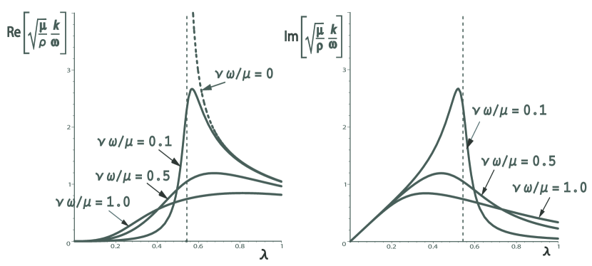
Figure 1: Dimensionless slowness and damping factor for a surface wave with real frequency in a Mooney-Rivlin viscoelastic solid subject to plane strain. The analysis shows that the half-space becomes unstable when compressed by more than about 46% (vertical asymptote) and this confines the validity of the curves to the right of the vertical dashed line.

When we take either $s_{2}=s_{2}^{\pm}$ as the root from (91), we find that the conditions (75), (76) cannot be satisfied simultaneously. Hence, there is only one possibility for a surface wave to propagate over a deformed viscoelastic Mooney-Rivlin solid, that which tends to the Rayleigh surface wave solution when the viscosity tends to zero. This is in accord with the results of Romeo [26] in linear elasticity (no finite pre-deformation).

5.2 Complex frequency, complex wave number

When we allow both the frequency and the wave number to be complex, we find that the imaginary part of $\omega$ is negative only in the range where $\lambda^{2}-\lambda^{-2}s_{2}^{2}\geq 0$, for $s_{2}=s_{2}^{0}=0.2956$; the other two roots $s_{2}^{\pm}$ of (91) do not yield any conclusion with respect to stability analysis. When $\lambda^{2}-\lambda^{-2}s_{2}^{2}<0$, i.e. when $\lambda<\lambda_{\text{cr}}=0.5436$, the imaginary part of $\omega$ is positive, indicating instability. When $\lambda=\lambda_{\text{cr}}=0.5436$, both the real and imaginary parts of $\omega$ are zero, as can be checked from the dispersion equation (92). The conclusion is then that the half-space becomes unstable when the complex speed $\omega/k$ is zero, just as in the purely elastic case. This is in accord with the correspondence principle of Biot [4].

References

• [1] S. Antman and T. Seidman, Large shearing motions of nonlinearly viscoelastic slabs Bull. Tech. Univ. Istanbul 47 (1994), 41–56.
• [2] M.F Beatty and Z. Zhou, Universal motions for a class of viscoelastic materials of differential type Continuum Mechanics and Thermodynamics 3 (1991), 169–191.
• [3] M.A. Biot, Surface instability of rubber in compression Appl. Sci. Research A12 (1963), 168–182.
• [4] M.A. Biot, Internal instability of anisotropic viscous and viscoelastic media under initial stress J. Franklin Inst. 279 (1965), 65–82.
• [5] Ph. Boulanger and M. Hayes, Bivectors and Waves in Mechanics and Optics Chapman & Hall, London, 1993.
• [6] P.K. Currie, M.A. Hayes and P.M. O’Leary, Viscoelastic Rayleigh waves Quart. Appl. Math. 35 (1977), 35–53.
• [7] P.K. Currie and P.M. O’Leary, Viscoelastic Rayleigh waves II Quart. Appl. Math. 36 (1978), 445–454.
• [8] M. Destrade and G. Saccomandi, Finite amplitude inhomogeneous waves in Mooney-Rivlin viscoelastic solids Wave Motion 40 (2004), 251–262.
• [9] M. Destrade and G. Saccomandi, On finite amplitude elastic waves propagating in compressible solids Physical Review E 72 (2005), 016620.
• [10] M. Destrade and G. Saccomandi, Creep, recovery, and waves in a nonlinear fiber-reinforced viscoelastic solid SIAM Journal on Applied Mathematics 68 (2007), 80–97.
• [11] M.A. Dowaikh and R.W. Ogden, On surface waves and deformations in a pre-stressed incompressible elastic solid IMA J. Appl. Math. 44 (1990), 261–284.
• [12] M. Fatemi, A. Manduca and J.F. Greenleaf, Imaging elastic properties of biological tissues by low-frequency harmonic vibration Proc. IEEE 91 (2003), 1503–1519.
• [13] J.N. Flavin, Surface waves in pre-stressed Mooney material Q. J. Mech. Appl. Math. 16 (1963), 441–449.
• [14] J.F. Greenleaf, M. Fatemi and M. Insana, Selected methods for imaging elastic properties of biological tissues Annu. Rev. Biomed. Eng. 5 (2003), 57 -78.
• [15] A.E. Green and J. E. Adkins, Large Elastic Deformations and Non-Linear Continuum Mechanics University Press, Oxford 1960.
• [16] M.A. Hayes and R.S. Rivlin, Propagation of small amplitude waves in a deformed viscoelastic solid I J. Acoust. Soc. Am. 46 (1969), 610–616.
• [17] M.A. Hayes and R.S. Rivlin, Propagation of small amplitude waves in a deformed viscoelastic solid II J. Acoust. Soc. Am. 51 (1972), 1652–1663.
• [18] M.A. Hayes and R.S. Rivlin, Longitudinal waves in a linear viscoelastic material ZAMP 23 (1972), 153–156.
• [19] M.A. Hayes and R.S. Rivlin, A class of waves in a deformed viscoelastic solid Q. Appl. Math. 30 (1972), 363–367.
• [20] M.A. Hayes and R.S. Rivlin, Plane waves in linear viscoelastic materials Quart. Appl. Math. 32 (1974), 113–121.
• [21] M.A. Hayes and G. Saccomandi, Finite amplitude transverse waves in special incompressible viscoelastic solids J. Elasticity 59 (2000), 213–225.
• [22] M.A. Hayes and G. Saccomandi, Finite amplitude waves superimposed on pseudoplanar motions for Mooney-Rivlin viscoelastic solids Int. J. of Nonlinear Mechanics 37 (2002), 1139–1146.
• [23] M.A. Hayes and G. Saccomandi, Antiplane shear motions for viscoelastic Mooney-Rivlin materials Quart. J. Mech. Appl. Math. 57 (2004), 379–392.
• [24] P.R. Hoskins, Physical properties of tissues relevant to arterial ultrasound imaging and blood velocity measurement Ultrasound Med. Biol. 33 (2007), 1527- 1539.
• [25] L.D Landau and E.M. Lifschitz, Theory Of Elasticity 3d revised version Elsevier 1984.
• [26] M. Romeo, Uniqueness of the solution to the secular equation for viscoelastic surface waves Appl. Math. Letters 15 (2002), 649–653.
• [27] K.R. Rajagopal and G. Saccomandi, Shear waves in some models of nonlinear viscoelasticity Quart. of Mech. and Appl. Math. 56 (2003), 311–326.
• [28] G. Saccomandi, Small amplitude waves in deformed Mooney-Rivlin viscoelastic solids Mathematics and Mechanics of Solids 10 (2005), 361–376.
• [29] A.L. Shuvalov and N.H. Scott, On the propagation of homogeneous viscoelastic waves Q. J. Mech. Appl. Math. 52 (1999), 405–417.
• [30] R. Sinkus, J. Bercoff, M. Tanter, J.-L Gennisson, C. El Khoury, V. Servois, A. Tardivon and M. Fink Nonlinear viscoelastic properties of tissue assessed by ultrasound Ultrasonics, Ferroelectrics and Frequency Control, IEEE Transactions 53 (2006), 2009–2018
• [31] C. Truesdell and W. Noll The Non-Linear Field Theories of Mechanics, Encyclopedia of Physics, Vol. III/3, Springer-Verlag 1965.