Width of the $0-\pi$ phase transition in diffusive magnetic Josephson junctions

Abstract

We investigate the Josephson current between two superconductors (S) which are connected through a diffusive magnetic junction with a complex structure (F_c). Using the quantum circuit theory, we obtain the phase diagram of $0$ and $\pi$ Josephson couplings for F_c being a IFI (insulator-ferromagnet-insulator) double barrier junction or a IFNFI structure (where N indicates a normal metal layer). Compared to a simple SFS structure, we find that the width of the transition, defined by the interval of exchange fields in which a $0-\pi$ transition is possible, is increased by insulating barriers at the interfaces and also by the presence of the additional N layer. The widest transition is found for symmetric F_c structures. The symmetric SIFNFIS presents the most favorable condition to detect the temperature induced $0-\pi$ transition with a relative width, which is five times larger than that of the corresponding simple SFS structure.

I Introduction

Ferromagnet-superconductor (FS) heterostructures feature novel and interesting phenomena, which have been active topics of investigation for more than half a century GKI04 ; BVE05 ; Buz05 . Meanwhile, Josephson structures comprising a ferromagnetic weak link have been studied extensively. The existence of the $\pi$-junction in a SFS structure is one of the most interesting phenomena which occurs for certain thicknesses and exchange fields of the F layer BKS77 ; Buz82 ; ROR01 ; ROVR01 ; KALG02 ; GABKL03 ; SBLC03 ; BPSB08 ; CBNB01 ; BVE01 ; RLF03 ; Cht04 ; BK91 ; Buz03 ; MZ06 ; VGKW08 ; LYS08 . This manifestation is due to the oscillatory behavior of the superconducting pair amplitude and the electronic density of states in the ferromagnet Buz00 ; ZB01 ; ZB02 . In a $\pi$-junction the ground state phase difference between two coupled superconductors is $\pi$ instead of $0$ as in the usual $0$-state SNS junctions. The existence of a $\pi$-state was predicted theoretically by Bulaevski et al. BKS77 and Buzdin et al. Buz82 , and has been first observed by Ryazanov et al. ROR01 . The transition from the $0$- to $\pi$-state is associated with a sign change of the critical current, $I_{c}$, which leads to a cusp-like dependence of the absolute values of $I_{c}$ on temperature. Later, the nonmonotonic temperature dependence of the critical current in diffusive contacts was observed in other experiments ROVR01 ; KALG02 ; GABKL03 ; SBLC03 ; BPSB08 and was attributed to the $0-\pi$ transition induced by the ferromagnetic exchange field. The $0-\pi$ transition has been studied theoretically by several authors in clean CBNB01 ; BVE01 ; RLF03 ; Cht04 and diffusive BK91 ; BVE01 ; Buz03 ; Cht04 ; MZ06 ; VGKW08 ; LYS08 Josephson contacts for different conditions and barriers at the FS interfaces.

An interesting application of a $\pi$-junction is a superconducting qubit as one of the most noticeable candidates for a basic element of quantum computing. Furthermore, $\pi$-junctions have been proposed as phase qubit elements in superconducting logic circuits IGF99 ; MOL99 ; BRG03 ; YTTM05 ; YTM06 . Also, a phase qubit in SIFIS junctions, in which the qubit state is characterized by the $0$ and the $\pi$ phase states of the junction, has recently been suggested NKS08 . Due to these exciting proposed applications, the detection of $0-\pi$ transitions with very high sensitivity is necessary. Investigating the phase diagrams of $0-\pi$ transitions CBNB01 ; LCE07 for different structures with different characteristics should make it possible to determine the most efficient control of the $0-\pi$ transition.

In this paper we investigate the width of the temperature-induced $0-\pi$ transition in a diffusive SF_cS junction. Here, F_c represents a complex ferromagnetic junction of length $L$, which consists of diffusive ferromagnetic and normal metallic parts as well as insulating barriers. We define the width of the transition as the interval of exchange fields, in which the temperature-dependent transition from the $0$- to $\pi$-phase is possible. We use the so-called quantum circuit theory (QCT), which is a finite-element technique for quasiclassical Green’s functions in the diffusive limit Naz94 ; Naz99 ; Naz05 . The QCT-description has the advantage, that it does not require to specify a concrete geometry. By a discretization of the Usadel equation Usa70 one obtains relations analogous to the Kirchhoff laws for classical electric circuit theory. These relations can be solved numerically by iterative methods and one obtains the quasiclassical Green’s function of the whole system. The QCT has been generalized to spin-dependent transport in Ref. HHNB02p, ; HHNB02, . We adopt the finding of this paper for FN contacts to handle our problem of the SF_cS contacts. We discretize the interlayer between the superconducting reservoirs into nodes. Following Refs. HHNB02, ; BN07, , every node in a ferromagnetic layer with specific exchange field is equivalent to a normal node connected to a ferromagnetic insulator reservoir which determines the exchange field. This similarity has been verified experimentally with EuO$|$Al$|$Al₂O${}_{3}|$Al junctions TTK86 . It has been found that the induced exchange-field of the EuO-insulator, which is responsible for spin-splitting in the measured density of states, was of the same order as its magnetization TTK86 . Also, the authors of Ref. HHNB02, have shown that the normalized density of states in the normal metal, which is connected to a superconductor and an insulator ferromagnet at its ends, is the same as the one for a BCS superconductor in the presence of a spin-splitting magnetic field GPTFS80 ; MT94 . This method allows us to calculate the Josephson current flowing through the SF_cS contact for an arbitrary length $L$ and all temperatures while fully taking into account the nonlinear effects of the induced superconducting correlations.

We investigate the width of the transition, $\Delta h$, for four different cases of SF_cS structures with ideally transparent FS-interfaces, symmetric SIFIS and asymmetric SIFS double barrier F-junctions, and more complicated SIFNFIS structures (where I and N denote, respectively, insulating barrier and normal metal). For a fixed length $L$, all these systems show several transition lines in the phase diagram of $T/T_{c}$ and $h/T_{c}$. Higher order transitions occur at large exchange fields $h$. We find that higher order transitions are wider than the first transition. Also, decreasing the contact length $L$ leads to a widening of the transitions and, at the same time, to an increasing of the exchange field, $h_{in}$, at which the transition starts. Nevertheless, the relative width of the transition, given by the ratio $\Delta h/h_{in}$, decreases.

For the SIFIS structure we show that the existence of the I-barriers at the FS interfaces broadens the $0-\pi$ transitions and, hence, improves the conditions to detect such transitions. In addition, we find that a symmetric double barrier structure with the two barriers having the same conductance shows wider transitions than the corresponding asymmetric structure with the same total conductance but different conductances of the barriers. An even larger width of transitions can be achieved by including an additional normal metal part into F_c. This motivates our study of an SIFNFIS structure, for which relative width $\Delta h/h_{in}$ is in general larger than that of the corresponding SIFIS with the same total conductance and the mean exchange field of the F_c part.

The structure of this paper is as follows. In Sec. II, we introduce the model and basic equations, which are used to investigate the SF_cS-Josephson junction. We introduce the finite-element description of our structures using quantum circuit theory technique. In Sec. III, we investigate phase diagrams of $0-\pi$ transitions for the SFS, SIFIS, and SIFNFIS structures. Analyzing our findings, we determine the most favorable conditions for an experimental detection of the $0-\pi$ transitions. Finally, we conclude in Sec. IV.

II Model and Basic Equations

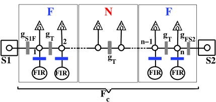
Figure 1: (Color online) Quantum circuit model of the SF_cS structure. The contact $F_{c}$ is discretized into $n$ nodes which are connected to each other by tunnel barriers of conductance $g_{T}$; $g_{S1F}$ and $g_{FS2}$ denote the conductances of S1F and FS2 interfaces, respectively. The inverse of the average level spacing, $\delta$, represents the leakage term due to a finite volume of a node; FIR represents a ferromagnetic insulating reservoir.

We consider a ferromagnetic SF_cS Josephson structure in which two conventional superconducting reservoirs are connected by a complex diffusive F_c junction. We investigate three cases of F_c: (i) a simple F layer with a homogeneous spin-splitting exchange field $h$ (SFS), (ii) a double barrier IFI structure, in which the F-layer is connected via I-barriers to the reservoirs (SIFIS), and (iii) an IFNFI junction composed of two ferromagnetic layers with the same length $L_{F}$ and the same exchange field and a normal metal with length $L_{N}$ in between such that $L=L_{N}+2L_{F}$ (SIFNFIS). We compare the width of the temperature-induced $0-\pi$ transitions for these three types of structures. In all cases F_c has the same length, total conductance, and the mean exchange field $h$.

In our approach, we make use of the quantum circuit theory which is a finite-element theory technique for quasiclassical Green’s function method in diffusive limit Naz94 ; Naz99 ; Naz05 . In this technique, each part of the structure is represented by a node which is connected to other nodes or superconductor/ferromagnet reservoirs HHNB02 . Green’s functions are calculated by using balance equations for matrix currents entering from the connectors, which is described in terms of its transmission properties and Green’s functions of the nodes forming it, to each node. For calculations we follow the procedure similar to that of Ref. BN07, . We discretize the conducting part of $F_{c}$ into $n$ nodes as presented in Fig. 1. A node in the ferromagnetic part will be presented by a normal-metal node connected to a ferromagnetic insulating reservoir (FIR) which induces an exchange field equal to the exchange field of the ferromagnetic part at the place of the node.

Each of the superconducting reservoirs is assumed to be a standard BCS-superconductor. Our circuit connecting those reservoirs consists of different types of nodes in F_c. One type are the normal nodes in the middle of F_c, each of which is connected to two neighboring nodes which are either normal nodes or F nodes. Another type are F nodes placed at the two ends of F_c, where each of them, in addition to its connection to two neighboring nodes, is connected to FIR as well and, hence, feels the exchange field directly. As can be seen in Fig. 1, each of the two neighboring nodes of a F node can be another F node, an N node, or a superconducting node. We denote the conductances of the tunnel barriers at S1F and FS2 interfaces by $g_{S1F}$ and $g_{FS2}$, respectively. Also, $g_{T}$ represents the conductance of the tunnel barrier between each two nodes inside $F_{c}$; $g_{T}$ is determined by $g_{F_{c}}$, the total conductance of $F_{c}$, excluding the conductances of the barriers at the interfaces $(n-1)/g_{T}=(1/g_{F_{c}})-(1/g_{S1F}+1/g_{FS2})$. In general, a node $i$ is characterized by a Green’s function $\check{G}_{i}$, which is an energy-dependent $4\times 4$-matrix in the Nambu and spin spaces. Furthermore, all nodes in F_c are assumed to be coupled to each other by means of tunneling contacts. However, a finite volume of a node and the associated decoherence between electron and hole excitations are taken into account by the leakage matrix current which is proportional to the energy, $\epsilon$, and the inverse of the average level spacing in the node, $\delta$ Naz94 ; Naz99 .

For a structure with spin-dependent magnetic contacts and in the presence of F and S reservoirs, the matrix current was developed in Ref. HHNB02, . In the limit of tunneling contacts, which is our interest, the matrix current between two nodes $i,j$ is defined as HHNB02 ; HN05 ,

$$\check{I}_{i,j}=\frac{g_{i,j}}{2}[\check{G}_{i},\check{G}_{j}]+\frac{G_{MR}}{4}[\{(\vec{h}_{i}.\vec{\hat{\sigma}})\hat{\tau}_{3},\check{G}_{i}\},\check{G}_{j}]$$ (1)

$$\\ +[i\frac{G_{Q}}{\delta_{i}}(\vec{h}_{i}.\vec{\hat{\sigma}})\hat{\tau}_{3},\check{G}_{j}].$$

The first term demonstrates the usual boundary condition for a tunneling junction, where $g_{i,j}$ is the tunneling conductance of the contact between the two nodes. The second term exists due to the different conductances for different spin directions which leads to the spin polarized current through the contact. We assume this term to be negligible as, $G_{MR}\sim g^{\uparrow}_{i,j}-g^{\downarrow}_{i,j}\ll g_{i,j}$. Also, $G_{Q}\equiv e^{2}/2\pi\hbar$ is the quantum of conductance, $\vec{h}$ is the exchange field of the node, and $\vec{\sigma}$ and $\vec{\tau}$ are the vectors consisting of Pauli matrices in spin and Nambu space.

Using Eq. (1) for different matrix currents entering into a given node $i$, we apply the condition of current conservation to obtain the following balance equation,

$$[\sum_{j=i-1,i+1}\frac{g_{j,i}}{2}\check{G}_{j}+i\frac{G_{Q}}{\delta_{i}}(\vec{h}_{i}.\vec{\hat{\sigma}})\hat{\tau}_{3}-i\frac{G_{Q}}{\delta_{i}}\epsilon\hat{\tau}_{3}\hat{\sigma}_{0},\check{G}_{i}]=0.$$ (2)

Here, the first term represents the matrix currents from neighboring nodes $i-1,i+1$, which could be F, N or S. The second and third terms are, respectively, the exchange term and the leakage matrix current. Also, $\hat{\sigma_{0}}$ represents unit matrix in spin space.

We consider the case, in which the exchange field in the ferromagnetic parts of F_c is homogeneous and collinear. Then, it is sufficient to work with the $2\times 2$ matrix Green’s function of spin-$\sigma$ ($\sigma=\uparrow/\downarrow$) electrons in Nambu space. In the Matsubara formalism the energy $\varepsilon$ is replaced by Matsubara frequency $i\omega=i\pi T(2m+1)$) and the Green’s function has the form

$$\hat{G}=\left(\begin{array}[]{cc}G&F\\ F^{*}&-G\end{array}\right).$$ (3)

Neglecting the inverse proximity effect in the right and left superconducting reservoirs, we set the boundary conditions at the corresponding nodes S1 and S2 to the bulk values of the matrix Green’s functions:

$$\hat{G}_{1,2}=\frac{1}{\sqrt{\omega^{2}+\Delta^{2}}}\left(\begin{array}[]{cc}\omega&\Delta e^{\pm i\phi/2}\\ \Delta e^{\mp i\phi/2}&-\omega\\ \end{array}\right)\,.$$ (4)

Here $\Delta e^{\pm i\phi/2}$ are, respectively, the superconducting order parameters in the right and left superconductors, and $\phi$ is the phase difference. The matrix Green s function satisfies the normalization condition, $\hat{G}^{2}=\hat{1}$. The temperature-dependence of the superconducting gap $\Delta$ is modeled by the following formula Muh59 ; Bel99

$$\Delta=1.76T_{c}\textrm{tanh}(1.74\sqrt{\frac{T}{T_{c}}-1}).$$ (5)

We scale the size of F_c in units of the diffusive superconducting coherence length, $\xi_{S}=\sqrt{\xi_{0}l_{imp}}$ where $\xi_{0}=v_{F}/\pi\Delta_{0}$ with $v_{F}$ being the Fermi velocity and $\Delta_{0}=\Delta(T=0)=1.76T_{c}$, and $l_{imp}$ is the mean free path in the F-layer related to the diffusion coefficient via $D=v^{(F)}_{F}l_{imp}/3$. Two more scales that we use are $h/T_{c}$ and $T/T_{c}$, where $T_{c}$ is the critical temperature of S reservoirs. Also, the mean level spacing depends on the size of the system via the Thouless energy $E_{Th}=D/L^{2}\equiv g_{T}\delta/(n-1)G_{Q}$ (Planck and Boltzmann constants, $\hbar$ and $k_{B}$, are set to 1 throughout this paper).

In the absence of spin-flip scatterings, the balance equation, Eq. (2), is written for each spin direction separately for all $n$ nodes in F_c. This results in a set of equations for $n$ matrix Green’s functions of the nodes that are solved numerically by iteration. In our calculation we start with choosing a trial form of the matrix Green’s functions of the nodes, for a given $\phi$, $T$, and the Matsubara frequency $m=1$. Then, using Eq. (2) and the boundary conditions iteratively, we refine the initial values until the Green’s functions are calculated in each of $n$ nodes with the desired accuracy. Note that in general for any phase differennce $\phi$, the resulting Green’s functions vary from one node to another, simulating the spatial variation along the F_c contact. From the resulting Green’s functions we calculate the spectral current using Eq. (1) and obtain

$$I=\frac{T}{4e}(2\pi i)\sum_{\omega_{m}=-\infty}^{\omega_{m}=\infty}Tr(\hat{\tau}_{3}\hat{I}).$$ (6)

In the second step we set the next Matsubara frequency $m=2$, find its contribution to the spectral current, and continue to the higher frequencies until the required precision of the summation over $m$ is achieved. Finding the spectral current, for the given temperature and phase difference, enables us to obtain the dependence of the critical current $I_{c}$ on $T$. Finally, we increase the number of nodes, $n$, and repeat the above procedure until all the spectral currents for every temperature and phase difference reach the specified accuracy. We find that for typical values of the involved parameters, a mesh of 60 nodes is sufficient to obtain $I_{c}$ through the diffusive F_c structure with an accuracy of $10^{-3}$ across the whole temperature range.

III Results and Discussions

¿From the numerical calculations, described above, we have obtained the phase diagram of $0-\pi$ transition in the plane of $h/T_{c}$ and $T/T_{c}$. We analyze the width of $0-\pi$ transitions for the SFS, symmetric SIFIS and asymmetric SIFS double barrier junctions, and SIFNFIS structures.

Concerning such transitions, the width $\Delta h$ defines the interval of the $h$, in which a temperature-induced transition occurs. We compare relative width, the ratio $\Delta h/h_{in}$, of different structures, where $h_{in}$ is the exchange field in which the transition starts (see Fig. 2a). In practice, we fix the size of the structures, $L/\xi_{s}$, and then vary the value of $h/T_{c}$ for detecting the change in the sign of the critical supercurrent as the transition occurs. We expect that the detection of a $0-\pi$ transition can be more feasible for the structure having larger $\Delta h/h_{in}$.

III.1 SFS structures

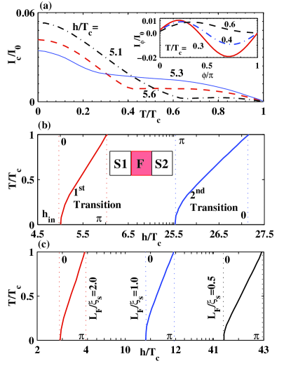
Figure 2: (a) (Color online) Normalized critical current, $I_{c}/I_{0}$, versus temperature for a SFS structure with the length $L_{F}/\xi_{s}=1.5$ and different exchange fields $h/T_{c}$. The inset shows the current-phase characteristic for $h/T_{c}=5.1$ in the vicinity of the $0-\pi$ transition temperature. (b) The corresponding $0-\pi$ phase diagram showing the phase boundaries up to the second transition. (c) Phase diagram of the first $0-\pi$ transition for different length of the junction $L_{F}/\xi_{s}$.

First, we consider the SFS structure. Figure. 2a presents the typical 0-$\pi$ transitions for such a junction with $L/\xi_{s}=1.5$, where the supercurrent is scaled in units of $I_{0}=(\pi/2)\Delta_{0}/eR_{F_{c}}$. Here, $R_{F_{c}}$ is the total resistance of F_c. We observe that the nonzero supercurrent at the transition point is larger when the transition temperature is lower. Also, the phase diagram is shown in Fig. 2b in the vicinity of the first and the second $0-\pi$ transitions. At the first transition the junction goes from the $0$- to the $\pi$-state starting at $h_{in}$ and $T=0$. Increasing $h$, the transition temperature increases toward $T_{c}$ and above the value $h=h_{in}+\Delta h$, the junction will be in $\pi$ state at all temperatures. Increasing $h$ further, the junction stays at its $\pi$ state until the exchange field reaches the value at which the second transition starts (see Fig. 2b) where the junction changes back to a $0$-state. In principal, it is possible to go to the higher exchange fields to see higher transitions. However the amplitude of the supercurrent will be extremely small and difficult to detect experimentally.

We have observed that the second transition is always wider than the first one. In the case of Fig. 2b, the width of the first transition is nearly 0.65 of that of the second one. Furthermore, the relative width for first transition is 0.20, while the second transition has $\Delta h/h_{in}=0.06$. This finding can also be generalized to higher transitions. In brief, higher transitions are always associated with larger widths. In spite of having a smaller width, the first transition seems to be more feasibly detectable, since they have higher $\Delta h/h_{in}$.

Looking at the origin of the existence of $0-\pi$ transition, we can understand this finding. An oscillating behavior of the order parameter in a ferromagnetic layer makes the occurrence of different signs of order parameters of the superconductor reservoirs, possible. This effect, being in charge of the $\pi$-phase state, can be seen when the length of the ferromagnet is of the order of half-integer multiple of a period $2\pi\xi_{F}$, where $\xi_{F}$ is the ferromagnetic coherence length of the ferromagnet. In the diffusive limit when $h>>T_{c}$, this length is equal to $\xi_{F}=\sqrt{D/h}$. Hence, as $d\xi_{F}/dh$ is inversely proportional to the exchange field, when the exchange field becomes larger the rate of reduction of $\xi_{F}$ decreases and the system will remain longer in the region of transition.

Now let us consider the effect of the length of F on the width of the transition. In Fig. 2c, the width of the first transition for three lengths $L/\xi_{s}=0.5,1,2$ are compared. As mentioned above, the condition for the occurrence of the first transition is that the length $L$ becomes of the order of half-integer of the period. For a smaller $L$ this condition is fulfilled at larger $h$ which, in light of the above discussion, means a wider $0-\pi$ transition. This can be seen easily in Fig.  2c. Note that the transition between the two states always starts from lower temperatures.

III.2 SIFIS, SIFS, and SIFNFIS structures

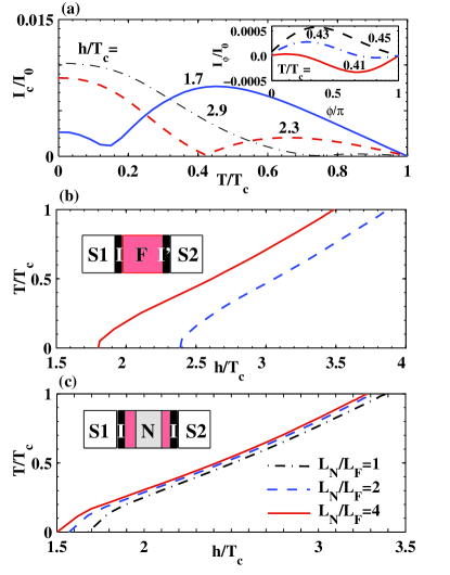
Figure 3: (a) (Color online) Normalized critical current, $I_{c}/I_{0}$, versus temperature of a symmetric SIFIS structure with $g_{S1F}=g_{FS2}=0.018g_{T}$ for different $h/T_{c}$, when $L_{F}/\xi_{s}=1.5$. The inset shows the corresponding $I-\phi$ characteristic for $h/T_{c}=2.0$ in the vicinity of the $0-\pi$ transition temperature. (b) Phase diagram of $0-\pi$ transition for a symmetric SIFIS structure with $g_{S1F}=g_{FS2}=0.018g_{T}$ (solid line) and the corresponding asymmetric structure (dashed line) with $g_{S1F}=0.1g_{FS2}=0.1g_{T}$, when $L_{F}/\xi_{s}=1.5$. (c) The same as (b) but for a symmetric SIFNFIS structure of $g_{S1F}=g_{FS2}=0.018g_{T}$ with $L/\xi_{s}=1.5$ and various $L_{N}/\L_{F}$.

Next, we examine the effect of putting insulating barriers at FS-interfaces. In Fig. 3a, the typical 0-$\pi$ transitions for SIFIS structure with $L/\xi_{s}=1.5$ is shown. As one can see, the presence of barriers adjusts the nonzero minimum cusp appearing in the diagram of the critical current versus temperature. Figure. 3b manifests the $0-\pi$ phase diagram for the symmetric SIFIS (solid curve) and the asymmetric SIFS (dashed curve) double barrier F_c. Compared to the corresponding SFS with $\Delta h/h_{in}=0.2$, these structures show wider transitions with $\Delta h/h_{in}=0.93$ for SIFIS of the conductance of the barrier $g_{S1F}=g_{FS2}=0.018g_{T}$, and $\Delta h/h_{in}=0.61$ for SIFS of $g_{S1F}=0.1g_{FS2}=0.1g_{T}$.

We have found that the strength of the barriers between the FS junctions is the most important parameter for determining the width of $0-\pi$ transitions. On the one hand, as the barriers get stronger the width of transitions becomes wider. This widening will be more pronounced for short length structures. On the other hand, for these structure the transition will start from a lower exchange field in comparison with the corresponding SFS systems.

Considering the effect of the relative values of the conductances of the two barrier, a symmetric SIFIS structures shows broader transitions as compared to the asymmetric SIFS structure with the same total conductance, as can be seen in Fig. 3b.

In addition, considering the displacement of the barrier in a S1I₁F₁I₂F₂S2 hybrid structures, we have found that the effect of barriers becomes more important as the barriers are closer to the ends of F_c, so that, SIFIS is the most optimal structure regarding the width of the transitions.

Finally, we have investigated the width of the $0-\pi$ transitions for SIFNFIS structures. The phase diagrams are shown in Fig. 3c for junctions with $L/\xi_{s}=1.5$ and various values of the length of the N part, $L_{N}$. We see that, putting a normal metal between the ferromagnets while keeping the magnetization of the system constant increases the width of the transition somewhat. This can be due to stronger penetration of superconductivity near the FS boundaries where the density of magnetization is larger which strengthens the mean effect of exchange field.

We have also observed that increasing $L_{N}$ leads to a further increase in the width of transition. However, this increase is saturated at higher lengthes. While the width for SIFNFIS structures of $L_{N}=2L_{F}$ is almost doubled compared to the SIFS structure, it is increased only few percent by increasing $L_{N}$ from $2L_{F}$ to $4L_{F}$ (see Fig. 3c).

It is worth to note that taking the absolute width $\Delta h$ as measure of the feasibility to detect the temperature-induced $0-\pi$ transition will lead to similar results as those of obtained above by considering the relative width $\Delta h/h_{in}$. However, the definition by $\Delta h/h_{in}$ seems to be more appropriate, since higher feasibility of detection requires not only larger $\Delta h$, but also smaller $h_{in}$ in order to have weaker exchange-induced suppression of the supercurrent.

IV Conclusion

In conclusion, we have investigated the width of $0-\pi$ transitions for various diffusive ferromagnetic Josephson structures (F_c) made of feromagnetic (F) and normal metal (N) layers and the insulating barrier (I) contacts. We have performed numerical calculations of the Josephson current within the quantum circuit theory technique which takes into account fully nonlinear proximity effect. The resulting phase diagram of $0$ and $\pi$ Josephson couplings in the plane of $T/T_{c}$ and $h/T_{c}$ shows that the existence of the insulating barrier contacts and the normal metal inter-layer leads to the enhancement of the relative width of the temperature induced transition. The relative width is parameterized by the ratio $\Delta h/h_{in}$ with $\Delta h$ and $h_{in}$ being, respectively, the exchange field interval upon which the transition is possible and the initial value of $h$ at which the transition occurs at $T=0$. We have also observed that while the conductance, the magnetization, and the length of the F_c junction are kept fixed, symmetric structures with the same barrier contacts and the same F layers in a SIFNFIS structure show larger relative width of the transition compared to that of the asymmetric structures. Among the studied structures, a symmetric SIFNFIS junction have the highest $\Delta h/h_{in}$, which makes it more practicable for highly sensitive detection of the temperature-induced $0-\pi$ transition.

- (1) A.A. Golubov, M.Yu. Kupryanov and E. Il’ichev, Rev. Mod. Phys. 76, 411 (2004).
- (2) F. S. Bergeret, A. F. Volkov, and K. B. Efetov, Rev. Mod. Phys. 77, 1321 (2005).
- (3) A. I. Buzdin, Rev. Mod. Phys. 77, 935 (2005).
- (4) A. Buzdin, Phys. Rev. B 62, 11377 (2000).
- (5) M. Zareyan, W. Belzig, and Yu.V. Nazarov, Phys. Rev. Lett. 86, 308 (2001).
- (6) M. Zareyan, W. Belzig, and Yu.V. Nazarov, Phys. Rev. B 65, 184505 (2002).
- (7) L. N. Bulaevskii, V. V. Kuzii, and A. A. Sobyanin, JETP Lett. 25, 90 (1977).
- (8) A. I. Buzdin, L. N. Bulaevskii, and S. V. Panyukov, JETP Lett. 35 187 (1982).
- (9) V. V. Ryazanov, V. A. Oboznov, A. Yu. Rusanov, A. V. Veretennikov, A. A. Golubov and J. Aarts, Phys. Rev. Lett. 86 2427 (2001).
- (10) V. V. Ryazanov, V. A. Oboznov, A. V. Veretennikov, A. Yu. Rusanov, Phys. Rev. B 65 020501(R) (2001).
- (11) T. Kontos, M. Aprili, J. Lesueur, F. Genêt, B. Stephanidis, and R. Boursier, Phys. Rev. Lett. 89 137007 (2002).
- (12) W. Guichard, M. Aprili, O. Bourgeois, T. Kontos, J. Lesueur, and P. Gandit, Phys. Rev. Lett. 90 167001 (2003).
- (13) H. Sellier, C. Baraduc, F. Lefloch, and R. Calemczuk, Phys. Rev. B 68, 054531 (2003).
- (14) A. A. Bannykh, J. Pfeiffer, V. S. Stolyarov, I. E. Batov, V. V. Ryazanov, M. Weides, arXiv:0808.3332 (2008)
- (15) N. M. Chtchelatchev, W. Belzig, Yu. V. Nazarov, and C. Bruder, JETP Lett. 74, 323 (2001) [Pis’ma v Zh. Eksp. Teor. Fiz. 74, 357 (2001)].
- (16) Z. Radovic, N. Lazarides, and N. Flytzanis, Phys. Rev. B 68, 014501 (2003).
- (17) N. M. Chtchelkatchev, JETP Letters 80, 743 (2004) [Pis’ma v Zh. Éksp. i Teor. Fiz. 80, 875 (2004)].
- (18) F. S. Bergeret, A. F. Volkov, and K. B. Efetov, Phys. Rev. B 64, 134506 (2001)
- (19) A. I. Buzdin and M. Yu. Kupriyanov, Pis ma Zh. Eksp. Teor. Fiz. 53, 308 (1991) [JETP Lett. 53, 321 (1991)].
- (20) A. Buzdin, Pis ma Zh. Eksp. Teor. Fiz. 78, 1073 (2003)[JETP Lett. 78, 583 (2003)].
- (21) G. Mohammadkhani and M. Zareyan, Phys. Rev. B 73, 134503 (2006).
- (22) A. S. Vasenko, A. A. Golubov, M. Yu. Kupriyanov, and M. Weides, Phys. Rev. B 77, 134507 (2008)
- (23) J. Linder, T. Yokoyama, and A. Sudbø, Phys. Rev. B 77, 174514 (2008).
- (24) L. B. Ioffe, V. B. Geshkenbein, M. V. Feigelman, A. L. Fauchere, and G. Blatter, Nature (London) 398, 679 (1999).
- (25) J. E. Mooij, T. P. Orlando, L. Levitov, L. Tain, C. H. van der Wal, and S. Lioyd, Science 285, 1036 (1999).
- (26) A. J. Berkley, H. Xu, R. C. Ramos, M. A. Gubrud, F. W. Strauch, P. R. Johnson, J. R. Anderson, A. J. Dragt, C. J. Lobb, and F. C. Wellstood, Science 300, 1548 (2003).
- (27) T. Yamashita, K. Tanikawa, S. Takahashi, and S. Maekawa, Phys. Rev. Lett. 95, 097001 (2005).
- (28) T. Yamashita, S. Takahashi, and S. Maekawa, Appl. Phys. Lett. 88, 132501 (2006).
- (29) T. W. Noh, M. D. Kim, and H. S. Sim, arXiv:0804.0349v1 (2008)
- (30) T. Lofwander, T. Champel, M. Eschrig, Phys. Rev. B 75, 014512 (2007).
- (31) Yu.V. Nazarov, Phys. Rev. Lett. 73, 1420 (1994).
- (32) Yu.V. Nazarov, Superlattices and Microstructures 25, 1221 (1999).
- (33) Yu.V. Nazarov, Quantum Transport and Circuit Theory (Handbook of Theoretical and Computational Nanotechnology, Micheal Rieth and Wolfram Schommers, eds, American Scientific Publishers, 2005), Vol. 1
- (34) K.D. Usadel, Phys. Rev. Lett. 25, 507 (1970).
- (35) D. Huertas-Hernando, Yu.V. Nazarov and W. Belzig, arXiv:0204116 (2002)
- (36) D. Huertas-Hernando, Yu.V. Nazarov and W. Belzig, Phys. Rev. Lett. 88, 047003 (2002).
- (37) V. Braude and Yu. V. Nazarov, Phys. Rev. Lett. 98, 077003 (2007).
- (38) P. M. Tedrow, J. E. Tkaczyk and A. Kumar, Phys. Rev. Lett. 56, 1746 (1986).
- (39) W. J. Gallagher, D. E. Paraskevopoulos, P. M. Tedrow, S. Frota-Pessoa, and B. B. Schwartz, Phys. Rev. B 21, 962 (1980).
- (40) R. Meservey and P. M. Tedrow, Phys. Rep. 238, 173 (1994).
- (41) D. Huertas-Hernando and Yu.V. Nazarov, Eur. Phys. J. B 44, 373 (2005).
- (42) B. Mühlschlegel, Z. Phys., 155, 313 (1959).
- (43) W. Belzig, F. K. Wilhelm, C. Bruder, G. Schön, and A. D. Zaikin, Superlattices Microst. 25, 1251 (1999)