Test of the ATLAS pion calibration scheme in the ATLAS combined test beam

Abstract

Pion energy reconstruction is studied using the data collected during the 2004 ATLAS combined test beam. The strategy to extract corrections for the non-compensating nature of the ATLAS calorimeters for dead material losses and for leakage effects is discussed and assessed. The default ATLAS strategy based on a weighting technique of the energy deposits in calorimeter cells is presented and compared to a novel technique exploiting correlations among energy deposited in calorimeter layers.

1 Introduction

Non-linearity and resolutions degradation in energy reconstruction of hadrons by calorimeters result from non-compensation effects compounded by unmeasured energy deposited in non-instrumented (dead) material. Calibration techniques are used to recover linearity and improve resolution.

In the year 2004 the ATLAS collaboration carried out a test-beam where a full central  slice of the ATLAS detector was exposed to beams of electrons and pions a large energy range. One of the main purposes of this combined test-beam was to test the ATLAS strategy to use a calibration based on simulation to reconstruct the correct energy of pions.

The general long-term ATLAS strategy to use simulation to calibrate the detector response to hadrons is shown in [1], while the quality of the simulation for the combined test beam data is discussed in [2]. The result of these two inputs is shown in the present report.

The experimental setup and the real and simulated data samples are briefly illustrated in sections 2 and 3. The pion calibration techniques are illustrated in section 4. The performance on simulation and data is discussed in terms of linearity and resolution in section 5.

2 Experimental setup

The 2004 ATLAS combined test beam is shown in the sketch of figure 1. It was composed of a full central slice of the ATLAS detector extending for about three units in pseudo-rapidity  and for 0.3 radians the azimuthal direction, $\phi$, around the beam axis. The central semiconductor pixel and strip detectors were housed in a bending magnet and followed by the straw-tube transition radiation tracker. The ATLAS central sampling calorimeters followed: one barrel module of the liquid argon-lead electromagnetic calorimeter (LAr) with accordion shape was housed in its cryostat and put in front of three hadronic iron-scintillator modules (Tile) stacked in the azimuthal direction, orthogonally to the incoming test beam axis.

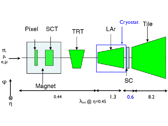
Figure 1: The experimental layout for the 2004 ATLAS combined test beam. See text for details.

The setup was exposed to beams of particles (pions, protons, electrons and muons) in the energy range 1 to 350 GeV. At $\eta$ = 0.45 the material in front of the calorimeters is estimated to consist of 0.44 $\lambda_{int}$  and the calorimetry stretches for about 9.5 $\lambda_{int}$ : 1.3 $\lambda_{int}$ for LAr and 8.2 $\lambda_{int}$ for Tile. The LAr cryostat accounts for additional 0.6 $\lambda_{int}$ in between the LAr and the Tile.

3 Data and simulation samples

The data consists of samples of events in which positive pions impinge on the experimental setup at $\phi$ = 0 and $\eta$ = 0.45. They are summarized in table 1.

Table 1: Properties of positive pion data samples used in the analysis. The sample fraction of proton events is also reported. At 180 GeV, pion events are selected from a sample of positron events.

Positive pion data samples
Selected events	Energy (GeV)	Proton contam. (%)
8000	20	0
15000	50	41
7000	100	59
5000	180	75

The pion beams are generated from proton primary beams extracted from the CERN SPS accelerator: the resulting proton contamination is measured by estimating the fraction of proton events that are necessary to reproduce the observed probability of generating a high energy hit in the transition radiation detector. The pion selection is documented in [2]. The proton contamination required simulation of samples of pions and protons in the range 15 to 230 GeV with GEANT 4.7 [3] using the QGSP_BERT physics [5] list and a consistent description of the test-beam set-up. The 4 million events simulated were split in two statistically independent sets of samples, the first one used for deriving simulation corrections and the second for testing the expected performance.

4 Pion calibration techniques

An incoming pion in the ATLAS detector causes a shower that is sampled by the seven calorimeter layers of the combined electromagnetic and hadronic sections. Any hadronic calibration scheme has to recover the intrinsic losses due to the invisible energy lost in nuclear interactions. Additional imperfections in the reconstruction also need to be accounted for: corrections are required for the imperfect energy collection of the clustering algorithm (out-of cluster) and incomplete shower containment (leakage of neutrons, muons and neutrinos). Finally corrections for energy deposits in non-instrumented material have an important role. In particular, in the ATLAS central region (barrel) a non-negligible amount of dead material is present between the electromagnetic and hadronic compartments i.e. in the midst of the longitudinal development of most hadronic showers.

Two calibration techniques are considered. The default ATLAS local hadronic calibration (LH in the following) is described in detail in [1]. A novel technique (described in section 4) is also considered: it is based on the use of correlations between the signals at the layer level, summing the clustered energy in each calorimeter longitudinal segment. It is called layer correlation calibration (LC in the following). The ansatz is that hadronic and electromagnetic energy deposits have different fluctuations properties and, consequently, variables that are sensitive to fluctuations in the total energy can be used both to derive all the corrections and improve the resolution of the total energy measurement.

The two techniques result in different outputs: LH produces calibrated clusters that will be used to form calibrated jets. On the other hand LC provides calibrated layer energies: such scheme is technically extendible to jets, but it will be aimed at calibrating the given jet energy depositions in a layer.

5 Performance of the hadronic calibration schemes

Performance is assessed in terms of linearity and relative resolution.

The total energy is fitted with a Gaussian in the [$\mu$- 2$\sigma$, $\mu$ + 2$\sigma$] interval where $\mu$ is the mean of the initial energy distribution and $\sigma$ is its standard deviation. Linearity is defined as the ratio of the expected fitted average to the beam energy as a function of the beam energy. Relative resolution is defined as the ratio of the fitted standard deviation to the fitted average as a function of the beam energy.

5.1 Expected linearity and resolution for the LH scheme

Linearity obtained with LH from simulated positive pion events is shown in the upper plot of figure 2. At the electromagnetic scale the typical linearity shape for non-compensating calorimeters is observed: about 75% of the beam energy is measured and the linearity ratio increases with beam energy due to the increasing electromagnetic fraction of the shower. The compensation weights recover about 10% of the total beam energy. The small out-of-cluster corrections account for about 1% of the beam energy. The remaining 10% is recovered by adding the dead material corrections. Linearity is finally recovered within 2% for beam energy larger than 20 GeV.

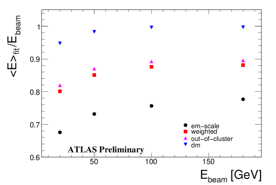
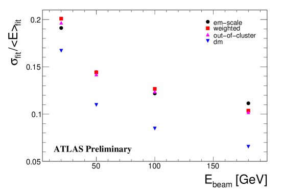
Figure 2: LH scheme: linearity (upper plot) and relative resolution (lower plot) for simulated positive pion events impinging on the test-beam setup at $\eta$ = 0.45. The various stages of correction are shown (see text for details).

The relative resolution is shown in the lower plot of figure 2. Dead material effects are expected to play a dominant role. The improvement in relative resolution deriving from suppressing the various fluctuations is expected to reach 11% to 40%.

5.2 LC scheme

The LC technique defines the total pion energy as the sum of clustered energy for each calorimeter layer. The event-by-event layer energy corrections are defined as a function of a specific pair of linear combinations of layer energies. Such combinations are the components of the seven-dimensional vector of layer energies along the vector space basis derived by a principal component analysis (PCA) [4]: the two components are used along the basis vectors whose associated PCA variance gives the largest contributions to the fluctuations of the total energy. Intuitively, the corrections depend on the “directions of largest independent fluctuations”, $E_{eig,i}$, where $i$ is an integer from one to seven.

Both the weights aimed at compensating the invisible energy and the corrections aimed at recovering dead material losses are derived as two dimensional look-up tables (seven for the layer energies, one for the dead material correction). For both types of tables, $E_{eig,0}$, the linear combination of layer energies with the largest contributions to the total energy fluctuation is one of the two dimension.

$E_{eig,1}$, the linear combination with the second largest contributions to the total energy fluctuation, is the second variable for the calculation of the compensation weights. The weight for a given layer energy in a given bin of the two dimensional table is defined as the average $E_{true}^{layer}/E_{rec}^{layer}$ over all the events in the bin . An example of the weight table for the first Tile layer is shown in figure 3. The separation between the high weight region, dominated by invisible energy, and the low-weight region, dominated by visible energy, is evident.

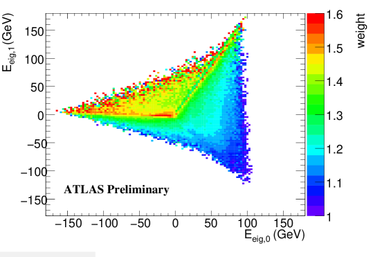
Figure 3: LC scheme: two dimensional look-up table of compensation weights for the first layer of the Tile hadronic calorimeter (see details in the text). Pions and protons samples are mixed to achieve a 41% proton contamination.

For the dead material correction, the second dimension is represented by, $E_{eig,2}$,the layer energy combination with the third largest contribution to the total energy fluctuations . The look-up table is shown in figure 4 where the high dead material correction region is well separated form the rest. The correction is derived as a function of the normalized linear combinations mentioned above (each combination is divided by the best estimate of the total energy) and it is expressed as a fraction of the total energy itself.

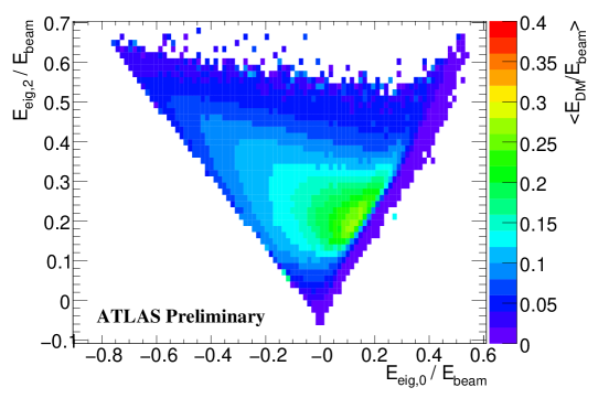
Figure 4: LC scheme: two dimensional look-up table of corrections for energy loss in dead material (as a fraction of total energy) between TileCal and LAr electromagnetic calorimeter (see details in the text). Pions and prootn samples are mixed to achieve a 41% proton contamination.

A small correction for the leakage, dead material energy losses upstream of the calorimeters and in between the first (presampler) and second (“strips”) LAr layers is calculated by a parametrization obtained from simulation as a function of the total energy estimate $E_{tot}$ .

An iterative procedure is then applied: a given total energy estimate provides a new dead material correction which can in turn be used to determine the total energy. A few iterations are required to obtain a stable result.

All look-up tables are filled by the full set of simulated samples from 15 to 230 GeV so as to reduce the beam energy dependence of the correction as much as possible.

5.3 Linearity and resolution for the LC scheme

In the case of the LC scheme a mix of pions and protons was used to derive the corrections and to simulate the data. The contamination values are those from table 1.

The upper plot of figure 5 shows the linearity obtained for both data and simulation: the agreement is within 2% at all stages of calibration. The resulting picture is similar to that outlined in section 5.1 for the LH scheme. The reconstruction at the electromagnetic scale is accounting for 75% of the beam energy. The compensation weights recover about 12% of the beam energy while the dead material correction accounts for about 10%. The dead material correction for losses between Tile and LAr represents about 80% of the total dead material corrections. The LC method recovers linearity within 3% over the whole energy range.

The relative resolution is shown the lower plot of figure  5. The simulation foresees a relative improvement of 17 to 24%: the data behave consistently showing an improvement of 17 to 21%. Even though the relative behaviour is the same, the simulation underestimates the resolution in the data by about 25%. GEANT4.9 [2] is expected to improve the data description.

5.4 LH vs LC scheme: linearity

Figure 6 shows the comparison for the resulting linearity when applying both calibration techniques to the same data set  The result is quite consistent: the linearity is recovered within 2 to 5% by both techniques.

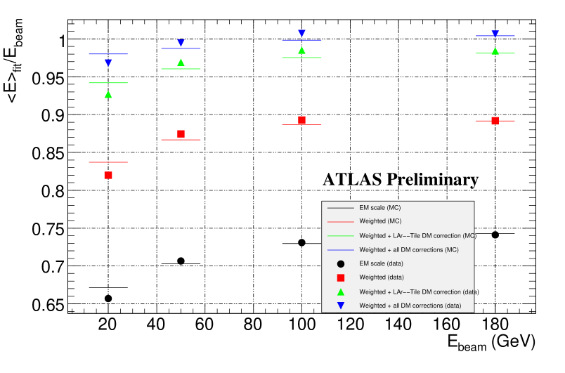
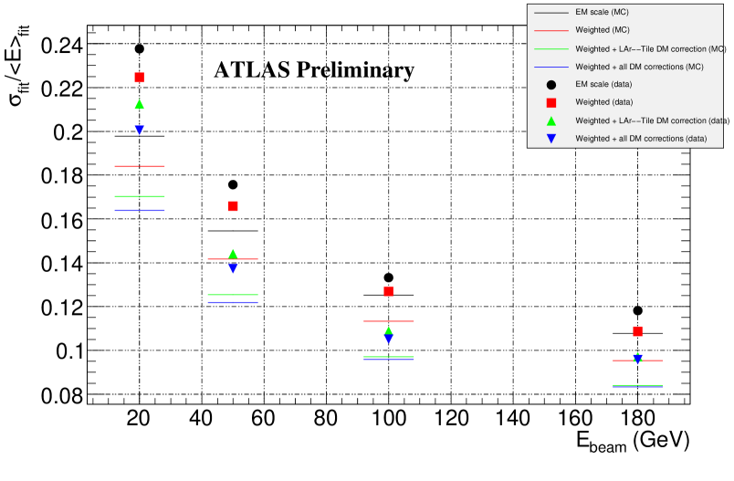
Figure 5: LC scheme: linearity (upper plot) and relative resolution (lower plot) for positive pion events impinging on the test-beam setup at $\eta$ = 0.45 at the various stages of correction (see text for details). Data are shown in filled symbols, simulated events are represented by horizontal lines.

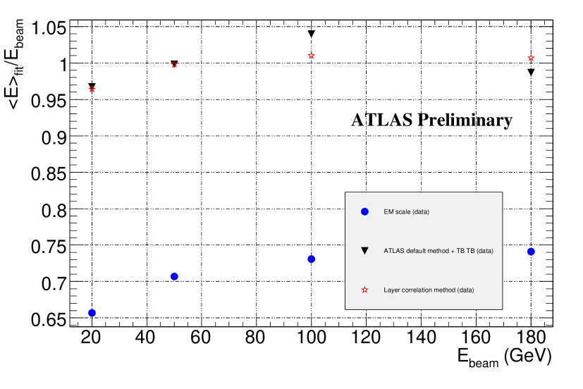
Figure 6: Comparison of linearity for the LH and LC schemes. Only the electromagnetic scale and the fully corrected scale are shown.

6 Conclusions

A simulation-based cell-weighting technique for hadronic signal calibration was applied to pion energy reconstruction in 2004 ATLAS combined test beam for beam energy in the range 20 to 180 GeV. A novel technique based on the correlation amongst layer energies was also used.

The linearity of response to charged pions is recovered within 2 to 5% by both approaches in good agreement between data and simulation; compensation weights and dead material effects have similar impact. According to simulation, the relative energy resolution is expected to improve (by 20-30% to 40%). LC actually achieves an improvement of 17 to 21%. Simulation underestimates data resolution by 10 to 25%; dead material effects are dominant.

Data-simulation discrepancies at the electromagnetic scale keep their size at all stages of calibration, thus simulation performance is the limiting factor.

The essential collaboration of Tancredi Carli, Karl-Johan Grahn and Peter Speckmayer is gratefully acknowledged.

References

References

- [1] Pospelov G 2008, these proceedings
- [2] Speckmayer P 2008, these proceedings
- [3] Agostinelli S et al. 2003 Nucl. Instr. and Meth. A 506 250-303 \nonumAllison J it et al. 2006 IEEE Transactions on Nuclear Science 53 No. 1 270-278.
- [4] Jackson J E 2005 A User’s Guide to Principal Components (Newark, NJ : Wiley) p 505
- [5] Guthrie M P, Alsmiller R G and Bertini H W 1968 Nucl. Instr. and Meth. A 66 29 \nonumGuthrie M P, Bertini H W 1971 Nucl. Phys. A 169 670