Effective pairing interaction in the two-dimensional Hubbard model
within a spin rotationally invariant approach

Abstract

We implement the rotationally-invariant formulation of the two-dimensional Hubbard model, with nearest-neighbors hopping $t$, which allows for the analytical study of the system in the low-energy limit. Both U(1) and SU(2) gauge transformations are used to factorize the charge and spin contributions to the original electron operator in terms of the corresponding gauge fields. The Hubbard Coulomb energy $U$ term is then expressed in terms of quantum phase variables conjugate to the local charge and variable spin-quantization axis, providing a useful representation of strongly correlated systems. It is shown that these gauge fields play a similar role as phonons in the BCS theory: they act as the “glue” for fermion pairing. By tracing out gauge degrees of freedom, the form of paired states is established and the strength of the pairing potential is determined. It is found that the attractive pairing potential in the effective low-energy fermionic action is non-zero in a rather narrow range of $U/t$.

I Introduction

Superconductivity represents a remarkable phenomenon where quantum coherence effects appear at macroscopic scale.bcs The quantum-mechanical phase of the electrons gains rigidity and as a result the properties of the quantum wave show up at the macro-macroscopic level. Thus, the superconducting properties are the manifestations of the spontaneous breakdown of one of the fundamental symmetries of matter, namely, the U(1) gauge symmetry. The discovery of the cuprate superconductors htsc has sparked a widespread interest in physics which goes beyond the traditional Fermi-liquid framework usually employed for understanding the effect of interactions in metals. The question of whether the pairing interaction in the cuprate superconductors should be characterized as arising from a pairing glue has recently been raised.and While there is a growing consensus that superconductivity in the high-$T_{c}$ cuprates arises from strong short-range Coulomb interactions between electrons rather than the traditional electron-phonon interaction, the precise nature of the pairing interaction remains controversial. In this context the Hubbard model is considered as essential physical system for treating superconductivity in the strongly correlated electron systems and has been intensively studied with a variety of methods such as quantum Monte-Carlo hirsch ; imada (QMC), exact diagonalization,fano ; moreo path-integral renormalization-group,kashima functional renormalization-group,metzner and various quantum cluster methods.cluster As a principal model describing the electronic correlation in the system, the Hubbard model has been used in many works to study the pairing instabilities which as usual are given by the second-order effective interaction with respect to the Coulomb interaction. In this context the structure of the pairing interaction, the two-dimensional (2D) Hubbard model, has been recently analyzed in Scalapino1 ; Scalapino2 ; Scalapino4 , where the dynamical cluster Monte Carlo approximation is applied to two-dimensional Hubbard model with nearest-neighbors hopping and on site Coulomb interaction. The Monte Carlo simulations have been also employed to study the phase separation and pairing in the doped two-dimensional Hubbard model.Scalapino3 However, the question whether the Hubbard model even supports superconductivity without additional interactions remains a subject of controversy. Different mean-field theories suggest conflicting ground-state order parameters and correlations, while finite-size QMC simulations for the doped 2D Hubbard model in the intermediate coupling regime of correlation energy $U$ support in general the idea of a spin-fluctuation-driven interaction mediating $d$-wave superconductivity. However, the fermion sign problem, limits these calculations to temperatures too high to study a possible transition. These simulations are also restricted to relatively small system sizes so that the off-diagonal long-range order has not been ascertained. For theoretical understanding of the mechanism of superconductivity in cuprates, the knowledge of bosons mediating the pairing is of pivotal importance. Here, the underlying attraction force appears very puzzling since it is hard to reconcile the microscopic attractive interaction with the completely repulsive bare electron-electron forces. This issue is closely related to the construction of the low-energy effective theory for the electronic system. A powerful tool for the quantitative investigation of microscopic models is provided by the study of effective theories: if one is able to single out the most relevant low-energy configurations, an effective theory can be extracted from the microscopic lattice Hamiltonian. This procedure is often implemented via the projective transformation, which results in removing of high-energy degrees of freedom and replacing them with kinematical constraints as exemplified, e.g., by the $t$-$J$ model.zhang In such approaches, the high-energy scale associated with the charge gap is argued to be irrelevant, hence the focus exclusively on the spin sector to characterize the Mott insulator. However, the charge-transfer nature of the cuprates plays an essential role in the doped systems,za so that with discarding charge degrees of freedom an important part of the physics may be lost. In the same spirit a detour from the strict projection program was recently proposed in a form of the “gossamer” superconductor,la recognizing the role of the double-occupancy charge configurations. However, the most interesting and relevant situation of strongly correlated systems, where magnetic as well as charge degrees of freedom interact, was until now investigated to a much lesser extent since it requires the treatment of the Hubbard Hamiltonian without imposing any restrictions on the correlation energy $U$.

In the present paper we study the emergence of the attractive pairing interaction in the two-dimensional Hubbard model by resorting to the analytical method that is deeply rooted in the inherent spin-rotational and gauge-charge symmetries of the model. To keep the spin-rotationally invariance, we write the action of the system using other bosonic and fermionic variables which are introduced with appropriate U(1) and SU(2) transformations. We construct a SU(2) spin-rotational and charge U(1) invariant theory using the electron operator factorization.Kopec ; Zaleski Furthermore, we derive the low-energy fermionic action that rests on the SU(2)-invariant character of the Hamiltonian and a consistent scheme of coherent states within a functional-integral formulation. We show that U(1) and SU(2) gauge fields (the collective high energy modes in the SC system) take over the task which was carried out by phonons in BCS superconductors and play the role of the “glue” that is responsible for the formation of the electron pairs. In this sense the present work charts a route from the microscopic Hubbard model on the square lattice to an effective lower energy action that exhibits pairing potential. The paper is organized as follows. Section II introduces the model and rotational invariant formulation. Section III describes charge and spin gauge transformations of fermions, which results in the phase-angular representation of strongly correlated electrons . Section IV is devoted to the evaluation of pairing interaction, while Sec. V discusses the effective fermionic action. We conclude with Sec. VI. Appendixes A, B and C contain miscellaneous results that pertain to the technical aspects of the work.

II Hubbard model in the rotating reference frame

The basic physics of strongly correlated electronic systems is the competition between the two tendencies of the electron to spread out as a wave and to localize as a particle, combined with magnetism. That is, the interplay of the spin and the charge degree of freedom is the central issue. These features are encoded in by the Hubbard Hamiltonian - the simplest yet nontrivial model for strongly correlated electrons. The relevance of this model for superconducting cuprates originates from the observation that the one -band Hubbard model tries to mimic the presence of the charge-transfer gap of cuprates by means of an effective value of the Coulomb repulsion. Thus, our starting point is the purely fermionic Hubbard Hamiltonian in the second-quantized form

$${\cal H}=-t\sum_{\langle{\bf r}{\bf r}^{\prime}\rangle,\alpha}[c^{\dagger}_{{\alpha}}({\bf r})c_{\alpha}({\bf r}^{\prime})+{\rm H.c.}]+\sum_{\bf r}Un_{\uparrow}({\bf r})n_{\downarrow}({\bf r}).$$ (1)

Here, $\langle{\bf r},{\bf r}^{\prime}\rangle$ runs over the nearest-neighbor (n.n.) sites, $t$ is the hopping amplitude, $U$ stands for the Coulomb repulsion, while the operator $c_{\alpha}^{\dagger}({\bf r})$ creates an electron with spin $\alpha=\uparrow(\equiv 1),\downarrow(\equiv 2)$ at the square lattice site ${\bf r}$. Furthermore, ${n}({{\bf r}})=n_{\uparrow}({\bf r})+n_{\downarrow}({\bf r})$ is the number operator, where ${n}_{\alpha}({{\bf r}})=c^{\dagger}_{\alpha}({\bf r})c_{\alpha}({\bf r})$. Usually, working in the grand canonical ensemble a term $-\mu\sum_{\bf r}{n}({\bf r})$ is added to ${\cal H}$ in Eq.(1) with $\mu$ being the chemical potential . We treat the problem of interacting fermions at finite temperature in the standard path-integral formalismnegele using Grassmann variables for Fermi fields, $c_{\alpha}({\bf r}\tau)$ depending on the “imaginary time” $0\leq\tau\leq\beta\equiv 1/k_{B}T$ (with $T$ being the temperature) that satisfy the anti-periodic condition $c_{\alpha}({\bf r}\tau)=-c_{\alpha}({\bf r}\tau+\beta)$, to write the path integral for the statistical sum ${\cal Z}=\int\left[{\cal D}\bar{c}{\cal D}{c}\right]e^{-{\cal S}[\bar{c},c]}$ with the fermionic action

$${\cal S}[\bar{c},c]={\cal S}_{B}[\bar{c},c]+\int_{0}^{\beta}d\tau{\cal H}[\bar{c},c],$$ (2)

that contains the fermionic Berry term

$${\cal S}_{B}[\bar{c},c]=\sum_{{\bf r}\alpha}\int_{0}^{\beta}d\tau\bar{c}_{\alpha}({\bf r}\tau)\partial_{\tau}{c}_{\alpha}({\bf r}\tau).$$ (3)

For the problem under study it is crucial to construct a covariant formulation of the theory, which naturally preserves the spin-rotational symmetry present in the Hubbard Hamiltonian. For this purpose, the density-density product in Eq.(1) we write, following Ref. schulz, , in a spin-rotational invariant way

$${\cal H}_{U}=U\sum_{{\bf r}}\left\{\frac{1}{4}{n}^{2}({{\bf r}}\tau)-\left[{\bf\Omega}({\bf r}\tau)\cdot{\bf S}({\bf r}\tau)\right]^{2}\right\},$$ (4)

where $S^{a}({\bf r}\tau)=\frac{1}{2}\sum_{\alpha\alpha^{\prime}}c^{\dagger}_{\alpha}({\bf r}\tau)\hat{\sigma}_{\alpha\alpha^{\prime}}^{a}c_{\alpha^{\prime}}({\bf r}\tau)$ denotes the vector spin operator ($a=x,y,z$) with $\hat{\sigma}^{a}$ being the Pauli matrices. The unit vector ${\bf\Omega}({\bf r}\tau)=[\sin\vartheta({\bf r}\tau)\cos\varphi({\bf r}\tau),\sin\vartheta({\bf r}\tau)\sin\varphi({\bf r}\tau),\cos\vartheta({\bf r}\tau)]$ written in terms of polar angles labels varying in space-time spin-quantization axis. Thus, the Hubbard Hamiltonian should not change its form under a rotation of the spin-quantization axis. This is not apparent in the standard form of the interaction in Eq.(1). The spin-rotation invariance is made explicit by performing the angular integration over ${\bf\Omega}({\bf r}\tau)$ at each site and time. By decoupling spin- and charge-density terms in Eq.(4) using auxiliary fields $\varrho({\bf r}\tau)$ and $iV({\bf r}\tau)$, respectively, we write down the partition function in the form,

$${\cal Z} = \int[{\cal D}{\bf\Omega}]\int[{\cal D}V{\cal D}{\varrho}]\int\left[{\cal D}\bar{c}{\cal D}c\right]\times$$ (5)

$$\times e^{-{\cal S}\left[{\bf\Omega},V,{\varrho},\bar{c},c\right]},$$

where$[{\cal D}{\bf\Omega}]\equiv\prod_{{\bf r}\tau_{k}}\frac{\sin\vartheta({\bf r}\tau_{k})d\vartheta({\bf r}\tau_{k})d\varphi({\bf r}\tau_{k})}{4\pi}$ is the spin-angular integration measure. The effective action reads as

$${\cal S}\left[{\bf\Omega},V,{\varrho},\bar{c},c\right] = \sum_{{\bf r}}\int_{0}^{\beta}d\tau\left[\frac{{\varrho}^{2}({\bf r}\tau)}{U}+\frac{V^{2}({\bf r}\tau)}{U}\right.$$ (6)

$$+ \left.iV({\bf r}\tau)n({\bf r}\tau)+2{\varrho}({\bf r}\tau){\bf\Omega}({\bf r}\tau)\cdot{\bf S}({\bf r}\tau)\right]$$

$$+ {\cal S}_{B}[\bar{c},c]+\int_{0}^{\beta}d\tau{\cal H}_{t}[\bar{c},c].$$

We would like to stress that the fermionic fields in Eq. (6) are the physical ones and not due to an enlargement of the Hilbert space like in a slave-boson treatment of the $t$-$J$ model.zhang As we see in Secs.IIIA-IIIC, the gauge fields will arise here by relating an SU(2) rotation in spin space and a vector on the two sphere ($S_{2}$).

III Charge and spin gauge transformations of fermions

The interaction term of the Hubbard Hamiltonian is quartic in fermion operators. This is a nonlinear problem which is not solvable except in some very special cases, such as one-dimensional systems. Thus, a standard approach is the mean-field approximation, sometimes called Hartree-Fock (HF)approximation, in which the quartic term is factorized in terms of a fermion bilinear times an auxiliary field, which is usually treated classically. However, HF theory will not work for a Hubbard model in which $U$ is the largest energy in the problem. One has to isolate strongly fluctuating modes generated by the Hubbard term according to the charge-U(1) and spin-SU(2) symmetries.

III.1 U(1) charge transformation

We swich mow from the particle-number representation to the conjugate phase representation of the electronic degrees of freedom. To this aim the second-quantized Hamiltonian of the model is translated to the phase representation with the help of the topologically constrained path-integral formalism. To this end we write the fluctuating “imaginary chemical potential” $iV({\bf r}\tau)$ as a sum of a static $V_{0}({\bf r})$ and periodic function $V({\bf r}\tau)=V_{0}({\bf r})+\tilde{V}({\bf r}\tau)$ using Fourier series,

$$\tilde{V}({\bf r}\tau)=\frac{1}{\beta}\sum_{n=1}^{\infty}[\tilde{V}({\bf r}\omega_{n})e^{i\omega_{n}\tau}+\text{c.c.}]$$ (7)

with $\omega_{n}=2\pi n/\beta$ ($n=0,\pm 1,\pm 2$) being the (Bose) Matsubara frequencies. Now, we introduce the U(1) phase field ${\phi}({\bf r}\tau)$ via the Faraday-type relation,

$$\dot{\phi}({\bf r}\tau)\equiv\frac{\partial\phi({\bf r}\tau)}{\partial\tau}=\tilde{V}({\bf r}\tau).$$ (8)

Since the homotopy group $\pi_{1}$[U(1)] forms a set of integers, discrete configurations of $\phi({\bf r}\tau)$ matter, for which $\phi({\bf r}\beta)-\phi({\bf r}0)=2\pi m({\bf r})$, where $m({\bf r})=0,\pm 1,\pm 2,\dots$ Thus the decomposition of the charge field $V({\bf r}\tau)$ conforms with the basic $m=0$ topological sector since $\int_{0}^{\beta}\dot{\phi}({\bf r}\tau)=\int_{0}^{\beta}\tilde{V}({\bf r}\tau)\equiv 0$. Furthermore, by performing the local gauge transformation to the new fermionic variables $f_{\alpha}({\bf r}\tau)$,

$$\left[\begin{array}[]{c}c_{\alpha}({\bf r}\tau)\\ \bar{c}_{\alpha}({\bf r}\tau)\end{array}\right]=\left[\begin{array}[]{cc}z({\bf r}\tau)&0\\ 0&\bar{z}({\bf r}\tau)\end{array}\right]\left[\begin{array}[]{c}f_{\alpha}({\bf r}\tau)\\ \bar{f}_{\alpha}({\bf r}\tau)\end{array}\right]$$ (15)

where the unimodular parameter $|z({\bf r}\tau)|^{2}=1$ satisfies $z({\bf r}\tau)=e^{i\phi({\bf r}\tau)}$, we remove the imaginary term $i\int_{0}^{\beta}d\tau\tilde{V}({\bf r}\tau)n({\bf r}\tau)$ for all the Fourier modes of the $V({\bf r}\tau)$ field, except for the zero frequency.

III.2 SU(2) spin transformation

In the above description, we focused on the charge degree of freedom of the electron. However, the electron has one more degree of freedom being the spin. The spin dominates the magnetic properties. The subsequent SU(2) transformation from $f_{\alpha}({\bf r}\tau)$ to $h_{\alpha}({\bf r}\tau)$ variables,

$$\left[\begin{array}[]{c}f_{1}({\bf r}\tau)\\ {f}_{2}({\bf r}\tau)\end{array}\right]=\left[\begin{array}[]{cc}\zeta_{1}({\bf r}\tau)&-\bar{\zeta}_{2}({\bf r}\tau)\\ \zeta_{2}({\bf r}\tau)&\bar{\zeta}_{1}({\bf r}\tau)\end{array}\right]\left[\begin{array}[]{c}h_{1}({\bf r}\tau)\\ {h}_{2}({\bf r}\tau)\end{array}\right]$$ (22)

with the constraint $|\zeta_{1}({\bf r}\tau)|^{2}+|\zeta_{2}({\bf r}\tau)|^{2}=1$ takes away the rotational dependence on ${\bf\Omega}({\bf r}\tau)$ in the spin sector. This is done by means of the Hopf map,

$${\bf R}({\bf r}\tau)\hat{\sigma}^{z}{\bf R}^{\dagger}({\bf r}\tau)=\hat{{\bm{\sigma}}}\cdot{\bf\Omega}({\bf r}\tau)$$ (23)

where

$${\bf R}({\bf r}\tau)=\left[\begin{array}[]{cc}\zeta_{1}({\bf r}\tau)&-\bar{\zeta}_{2}({\bf r}\tau)\\ \zeta_{2}({\bf r}\tau)&\bar{\zeta}_{1}({\bf r}\tau)\end{array}\right]$$ (24)

that is based on the enlargement from two sphere $S_{2}$ to the three sphere $S_{3}\sim{\rm SU}(2)$. The unimodular constraint can be resolved by using the parametrization

$$\zeta_{1}({\bf r}\tau) = e^{-{i}/{2}[\varphi({\bf r}\tau)+\chi({\bf r}\tau)]}\cos\left[\frac{\vartheta({\bf r}\tau)}{2}\right]$$

$$\zeta_{2}({\bf r}\tau) = e^{{i}/{2}[\varphi({\bf r}\tau)-\chi({\bf r}\tau)]}\sin\left[\frac{\vartheta({\bf r}\tau)}{2}\right]$$ (25)

with the Euler angular variables $\varphi({\bf r}\tau),\vartheta({\bf r}\tau)$ and $\chi({\bf r}\tau)$, respectively. Here, the extra variable $\chi({\bf r}\tau)$ represents the U(1) gauge freedom of the theory as a consequence of $S_{2}\to S_{3}$ mapping. One can summarize Eqs. (15) and (22) by the single joint gauge transformation exhibiting electron operator factorization

$$c_{\alpha}({\bf r}\tau)=\sum_{\alpha^{\prime}}z({\bf r}\tau){R}_{\alpha\alpha^{\prime}}({\bf r}\tau)h_{\alpha^{\prime}}({\bf r}\tau),$$ (26)

where ${\bf R}({\bf r}\tau)=e^{-i\hat{\sigma}_{z}\varphi({\bf r}\tau)/2}e^{-i\hat{\sigma}_{y}\vartheta({\bf r}\tau)/2}e^{-i\hat{\sigma}_{z}\chi({\bf r}\tau)/2}$ is a unitary matrix which rotates the spin-quantization axis at site ${\bf r}$ and time $\tau$. Equation(26) reflects the composite nature of the interacting electron formed from bosonic spinorial and charge degrees of freedom given by ${R}_{\alpha\alpha^{\prime}}({\bf r}\tau)$ and $z({\bf r}\tau)$, respectively, as well as remaining fermionic core part $h_{\alpha}({\bf r}\tau)$.

III.3 Fermionic sector

Anticipating that spatial and temporal fluctuations of the fields $V_{0}({\bf r})$ and $\varrho({\bf r}\tau)$ will be energetically penalized, since they are gaped and decouple from the angular and phase variables. Therefore, in order to make further progress we subject the functional in Eq.(6) to a saddle-point analysis with respect to non-fluctuating (static) fields and variables that fluctuations cost energy of the order of $U$. The expectation value of the static (zero-frequency) part of the fluctuating potential $V_{0}(r)$ in the charge sector we calculate by the saddle-point method to gives

$$V_{0}(r)=i\left(\mu-\frac{U}{2}n_{h}\right)\equiv i\bar{\mu}$$ (27)

where $\bar{\mu}$ is the chemical potential with a Hartree shift originating from the saddle-point value of the static variable $V_{0}({\bf r})$ with $n_{h}=n_{h\uparrow}+n_{h\downarrow}$ and $n_{h\alpha}=\langle\bar{h}_{\alpha}({\bf r}\tau)h_{\alpha}({\bf r}\tau)\rangle$. Similarly in the magnetic sector, a saddle-point evaluation of $\rho({\bf r})$ reproduces the conventional Hartree Fock equations for a commensurate antiferromagnet

$$\rho({\bf r}\tau)=(-1)^{\bf r}\Delta_{c}$$ (28)

where $\Delta_{c}=U\langle S^{z}({\bf r}\tau)\rangle$ sets the magnitude for the Mott-charge gap $\Delta_{c}\sim U/2$ for $U/t\gg 1$. The staggerization factor $(-1)^{\bf r}$ breaks the translation invariance by one site which remains by two sites. The term is readily handled by going to the reduced Brillouin zone.Zaleski Note that the notion antifferomagnetic here does not mean an actual long-range ordering - for this the angular spin-quantization variables governed by the rotational symmetry have to be ordered as well. To summarize, the fermionic sector is governed by the effective Hamiltonian

$${\cal H}_{\bf\Omega,\phi}=\sum_{{\bf r}}\Delta_{c}(-1)^{\bf r}[\bar{h}_{{\uparrow}}({\bf r}\tau)h_{\uparrow}({\bf r}\tau)-\bar{h}_{{\downarrow}}({\bf r}\tau)h_{\downarrow}({\bf r}\tau)]$$

$$-t\sum_{\langle{\bf r}{\bf r}^{\prime}\rangle,\alpha\gamma}\bar{z}({\bf r}\tau)z({\bf r}^{\prime}\tau)\left[{\bf R}^{\dagger}({\bf r}\tau){\bf R}({\bf r^{\prime}}\tau)\right]_{\alpha\gamma}\bar{h}_{{\alpha}}({\bf r}\tau)h_{\gamma}({\bf r}^{\prime}\tau)$$

$$-\bar{\mu}\sum_{{\bf r}\alpha}\bar{h}_{\alpha}({\bf r}\tau)h_{\alpha}({\bf r}\tau),$$ (29)

The chief merit of the gauge transformation in Eq.(26) is that we have managed to cast the Hubbard problem into a system of $h$ fermions submerged in the bath of strongly fluctuating U(1) and SU(2) gauge potentials (minimally coupled to fermions via hopping term) which mediate the interactions.

IV Pairing interaction

It is well known that the crucial point of BCS theory is the existence of an attractive interaction among electrons, where that phonons play the role of the “glue” that is responsible for the formation of Cooper pairs. Here, by integration out the bosonic scalar filed that represents phonons in the fermionic Hamiltonian, an effective attractive potential emerges. Now we show that U(1) and SU(2) emergent gauge fields (the collective high-energy modes in the Hubbard system) take over the task which was carried out by phonons in BCS superconductors. In a way similar to phonons these gauge fields couple to the fermion density-type term via the amplitude $t$, see Eq.(29),

$$-t\sum_{\langle{\bf r}{\bf r}^{\prime}\rangle,\alpha\gamma}\bar{z}({\bf r}\tau)z({\bf r}^{\prime}\tau)\left[{\bf R}^{\dagger}({\bf r}\tau){\bf R}({\bf r^{\prime}}\tau)\right]_{\alpha\gamma}\bar{h}_{{\alpha}}({\bf r}\tau)h_{\gamma}({\bf r}^{\prime}\tau)$$ (30)

Thus, in order to obtain an effective interaction among fermions we have to integrate out all the bosonic modes given by $\bar{z}({\bf r}\tau),z({\bf r}^{\prime}\tau)$ and ${\bf R}^{\dagger}({\bf r}\tau),{\bf R}({\bf r^{\prime}}\tau)$ fields. A major difference with respect to the BCS theory is that the variables to be integrated out are of tensorial nature since SU(2) modes carry spin index. To explicitly evaluate the effective interaction between fermions by tracing out the gauge degrees of freedom, we resort to the cumulant expansion To this end we write the partition function as ${\cal Z}=\int[{\cal D}{\bar{h}}{\cal D}h]e^{-{\cal S}[\bar{h},h]}$, where the effective fermionic action is

$$S_{eff}[\bar{h},h]=-\ln\int\left[{\cal{D}}\phi{\cal{D}}{\bf{\Omega}}\right]e^{-S\left[{\bf{\Omega}},\phi,\bar{h},h\right]}$$ (31)

The expression Eq.(31) generates a cumulant series when expanded with respect to the hopping variable $t$. The relevant second-order term that contains the quartic fermionic term becomes

$$S^{(2)}\left[\bar{h},h\right]=-{t^{2}}\sum_{\left\langle{\bf{r}}_{1}{\bf{r}}^{\prime}_{1}\right\rangle}\sum_{\left\langle{\bf{r}}_{2}{\bf{r}}^{\prime}_{2}\right\rangle}\int^{\beta}_{0}d\tau{d\tau^{\prime}}\left\langle\frac{}{}\bar{z}({\bf{r}}_{1}\tau)z({\bf{r}}^{\prime}_{1}\tau)\bar{z}({\bf{r}}_{2}\tau^{\prime})z({\bf{r}}^{\prime}_{2}\tau^{\prime})\frac{}{}\right\rangle_{\text{U(1)}}$$

$$\times\sum_{\alpha\alpha^{\prime}}\sum_{\gamma\gamma^{\prime}}\left\langle\frac{}{}\left[{\bf{R}}^{{\dagger}}({\bf{r}}_{1}\tau){\bf{R}}({\bf{r}}^{\prime}_{1}\tau)\right]_{\alpha\alpha^{\prime}}\left[{\bf{R}}^{{\dagger}}({\bf{r}}_{2}\tau^{\prime}){\bf{R}}({\bf{r}}^{\prime}_{2}\tau^{\prime})\right]_{\gamma\gamma^{\prime}}\right\rangle_{\text{SU(2)}}{\bar{h}_{\alpha}({\bf{r}}_{1}\tau)h_{\alpha^{\prime}}({\bf{r}}^{\prime}_{1}\tau)}\bar{h}_{\gamma}({\bf{r}}_{2}\tau^{\prime})h_{\gamma^{\prime}}({\bf{r}}^{\prime}_{2}\tau^{\prime})$$ (32)

where

$$\left\langle\dots\right\rangle_{\text{U(1)}}=\frac{\int\left[{\cal{D}}\phi\right]\dots e^{-S\left[\phi\right]}}{\int\left[{\cal{D}}\phi\right]e^{-S\left[\phi\right]}}$$ (33)

is the averaging over U(1) phase field while

$$\left\langle\dots\right\rangle_{\text{SU(2)}}=\frac{\int\left[{\cal{D}}{\bf{\Omega}}\right]e^{-S\left[{\bf{\Omega}}\right]}}{\int\left[{\cal{D}}{\bf{\Omega}}\right]e^{-S\left[{\bf{\Omega}}\right]}}$$ (34)

is the averaging over spin-angular variables. To proceed with the evaluation of the effective fermion-fermion interaction one has to develop procedures for effectuating both averages which involves calculation of the effective actions $S\left[\phi\right]$ and $S\left[{\bf{\Omega}}\right]$ in charge and spin sectors, respectively.

IV.1 U(1) average

The averaging in the charge sector is performed with the use of the U(1) phase action (see Appendix A).

$$S[\phi]=\sum_{\bf r}\int_{0}^{\beta}d\tau\left[\frac{\dot{\phi}^{2}({\bf r}\tau)}{U}+\frac{2\mu}{iU}\dot{\phi}({\bf r}\tau)\right]$$ (35)

that contains both the kinetic and Berry terms of the U(1) phase field in the charge sector. For the U(1) average in Eq.(32) we get

$$\left\langle\frac{}{}\bar{z}({\bf{r}}_{1}\tau)z({\bf{r}}^{\prime}_{1}\tau)\bar{z}({\bf{r}}_{2}\tau^{\prime})z({\bf{r}}^{\prime}_{2}\tau^{\prime})\frac{}{}\right\rangle_{\text{U(1)}}\approx\left(\delta_{{\bf{r}}_{1}{\bf{r}}^{\prime}_{1}}\delta_{{\bf{r}}_{2}{\bf{r}}^{\prime}_{2}}\right.$$

$$\left.+\delta_{{\bf{r}}_{1}{\bf{r}}^{\prime}_{2}}\delta_{{\bf{r}}^{\prime}_{1}{\bf{r}}_{2}}\right)e^{-\frac{U}{2}\left[|\tau-\tau^{\prime}|-{\left(\tau-\tau^{\prime}\right)^{2}}/{\beta}\right]}.$$ (36)

Specializing to the low-temperature limit

$$\lim_{\tau\rightarrow 0}\int^{\beta}_{0}d\tau^{\prime}e^{-|\tau-\tau^{\prime}|{U}/{2}}=\lim_{\tau\rightarrow 0}\left[\frac{2}{U}-\frac{2e^{-\beta{U}}}{2}\right]=\frac{2}{U},$$ (37)

we obtain the result for the U(1) phase average.

IV.2 SU(2) average

IV.2.1 Spin-angular action

The calculation of the SU(2) average is done with help of the effective action that involves the spin-directional degrees of freedom ${\bf\Omega}$, which important fluctuations correspond to rotations. This can be done by integrating out fermions ${\cal Z}=\int\left[{\cal D}{\bf\Omega}\right]e^{-{\cal S}[{\bf\Omega}]}$ where

$${\cal S}[{\bf\Omega}]=-\ln\int[{\cal D}\phi{\cal D}\bar{h}{\cal D}h]e^{-{\cal S}[\varphi,\phi,\vartheta,\bar{h},h]}$$ (38)

generates the low-energy action in the form ${\cal S}[{\bf\Omega}]=\mathcal{S}_{0}\left[\mathbf{\Omega}\right]+{\cal S}_{B}[{\bf\Omega}]+{\cal S}_{J}[{\bf\Omega}]$. The interaction term with the spin stiffness becomes

$${\cal S}_{J}[{\bf\Omega}]=\frac{J\left(\Delta\right)}{4}\sum_{\langle{\bf r}{\bf r}^{\prime}\rangle}\int_{0}^{\beta}d\tau{\bf\Omega}({\bf r}\tau)\cdot{\bf\Omega}({\bf r^{\prime}}\tau),$$ (39)

with the entiferromagnetic (AF) exchange coefficient

$$J(\Delta_{c})=\frac{4t^{2}}{U}(n_{\uparrow}-n_{\downarrow})^{2}\equiv\frac{4t^{2}}{U}\left(\frac{2\Delta_{c}}{U}\right)^{2}.$$ (40)

From Eq. (40) it is evident that for $U\to\infty$ one has $J(\Delta_{c})\sim\frac{4t^{2}}{U}$ since $\frac{2\Delta_{c}}{U}\to 1$ in this limit. Thus, in the strong-coupling limit, the half-filled Hubbard model maps onto the quantum Heisenberg model. In this limit the fermions are bound into localized spins. There is no motion of fermions, since they are suppressed by the gap for charge fluctuations. In general the AF-exchange parameter persists as long as the charge gap $\Delta_{c}$ exists. However, $J(\Delta_{c})$ diminishes rapidly in the $U/t\to 0$ weak-coupling limit. Because the gauge field is the phase factor arising in the inner product of quantum-mechanical states - the so-called connection in mathematical language - it is intimately related to the Berry phase term ${\cal S}_{B}[{\bf\Omega}]$ in the effective action. If we work in Dirac “north pole”gauge $\chi({\bf r}\tau)=-\varphi({\bf r}\tau)$ one recovers the familiar form

$${\cal S}_{B}[{\bf\Omega}]=\frac{\theta}{i}\sum_{{\bf r}}\int_{0}^{\beta}d\tau\dot{\varphi}({\bf r}\tau)[1-\cos\vartheta({\bf r}\tau)].$$ (41)

Here, the integral on the right-hand side of Eq. (41) has a simple geometrical interpretation as it is equal to a solid angle swept by a unit vector ${\bf\Omega}(\vartheta,\varphi)$ during its motion.auer The extra phase factor coming from the Berry phase requires some little extra care, since it will induce quantum-mechanical phase interference between configurations. In regard to the nonperturbative effects, we realized the presence of an additional parameter with the topological angle or so-called theta term

$$\theta=\frac{\Delta_{c}}{U}$$ (42)

that is related to the Mott gap. In the large-$U$ limit, one has $\Delta_{c}\to U/2$, so that $\theta\to\frac{1}{2}$ relevant for the half-integer spin. The kinetic-energy term in the spin sector becomes

$${\cal S}_{0}[{\bf\Omega}] = \sum_{\bf r}\int_{0}^{\beta}d\tau\left\{\right.\frac{1}{4{\cal E}_{s}}\left[{\dot{\vartheta}^{2}({\bf r}\tau)+\dot{\varphi}^{2}({\bf r}\tau)+\dot{\chi}^{2}({\bf r}\tau)}\right.$$ (43)

$$+ \left.{2}\dot{\varphi}({\bf r}\tau)\dot{\chi}({\bf r}\tau)\cos{\vartheta}({\bf r}\tau)\right]\left.\right\},$$

where $\mathcal{E}_{s}=1/\left(2\chi_{T}\right)$ and

$$\chi_{T}=\left\{\begin{array}[]{cc}\displaystyle\frac{1}{8J}&\,\,\,t\ll U\\ \displaystyle\frac{1}{2\pi}\frac{1}{t}\sqrt{\frac{t}{U}}&\,\,\,t\gg U\end{array}\right.$$ (44)

is the transverse spin suusceptibility.

IV.2.2 CP¹ representation

It the $CP^{1}$ representation, the spin-quantization axis can be conveniently written as

$$\mathbf{\Omega}\left(\mathbf{r}\tau\right)=\sum_{\alpha\alpha^{\prime}}\bar{\zeta}_{\alpha}\left(\mathbf{r}\tau\right)\bm{\sigma}_{\alpha\alpha^{\prime}}\zeta_{\alpha^{\prime}}\left(\mathbf{r}\tau\right).$$ (45)

As a consequence, all the terms in the spin action can be expressed as functions of unimodular $\zeta_{\alpha}\left(\mathbf{r}\tau\right)$ variables instead of angular variables, which are more complicated to be handled. Finally, the action assumes the form

$$\mathcal{S}\left[\bar{\bm{\zeta}},\bm{\zeta}\right]=\sum_{\mathbf{r}}\int_{0}^{\beta}d\tau\left\{2\chi_{T}\dot{\bm{\zeta}}\left(\mathbf{r}\tau\right)\cdot\dot{\bm{\zeta}}\left(\mathbf{r}\tau\right)\right.$$

$$-\left.\theta\left(-1\right)^{\mathbf{r}}\left[\bar{\bm{\zeta}}\left(\mathbf{r}\tau\right)\cdot\dot{\bm{\zeta}}\left(\mathbf{r}\tau\right)-\dot{\bar{\bm{\zeta}}}\left(\mathbf{r}\tau\right)\cdot\bm{\zeta}\left(\mathbf{r}\tau\right)\right]\right\}$$

$$-J\sum_{\left\langle\mathbf{r}\mathbf{r}^{\prime}\right\rangle}\int_{0}^{\beta}d\tau\bar{\mathcal{A}}\left(\mathbf{r}\tau\mathbf{r}^{\prime}\tau\right)\mathcal{A}\left(\mathbf{r}\tau\mathbf{r}^{\prime}\tau\right)$$ (46)

with the bond operators

$$\bar{\mathcal{A}}\left(\mathbf{r}\tau\mathbf{r}^{\prime}\tau\right)\mathcal{A}\left(\mathbf{r}\tau\mathbf{r}^{\prime}\tau\right)=-\frac{1}{4}\mathbf{\Omega}\left(\mathbf{r}\tau\right)\cdot\mathbf{\Omega}\left(\mathbf{r}^{\prime}\tau\right)+\frac{1}{4}$$

$$\mathcal{A}\left(\mathbf{r}\tau\mathbf{r}^{\prime}\tau\right)=\frac{\zeta_{\uparrow}\left(\mathbf{r}\tau\right)\zeta_{\downarrow}\left(\mathbf{r}^{\prime}\tau\right)-\zeta_{\downarrow}\mathbf{\left(\mathbf{r}\tau\right)}\zeta_{\uparrow}\left(\mathbf{r}^{\prime}\tau\right)}{\sqrt{2}}.$$ (47)

IV.2.3 Canonical transformation of CP¹ variables

In order to achieve a consistent representation of the underlying antiferromagnetic structure, it is unavoidable to explicitly split the degrees of freedom according to their location on sublattice A or B. Since the lattice is bipartite, allowing one to make the unitary transformation

$$\zeta_{\uparrow}({\bf r}\tau) \to -\zeta_{\downarrow}({\bf r}\tau)$$

$$\zeta_{\downarrow}({\bf r}\tau) \to \zeta_{\uparrow}({\bf r}\tau)$$ (48)

for sites on one sublattice, so that the antiferromagnetic bond operator becomes

$${\cal A}({\bf r}\tau{\bf r^{\prime}}\tau) \to {\cal A}^{\prime}({\bf r}\tau{\bf r^{\prime}}\tau)=\sum_{\alpha=1}^{2}\frac{\zeta_{\alpha}({\bf r}\tau)\zeta_{\alpha}({\bf r}^{\prime}\tau)}{\sqrt{2}}.$$ (49)

This canonical transformation preserves the unimodular constraint of the $CP^{1}$ fields. Biquadratic (four-variable) terms in the Lagrangian cannot be readily integrated in the path integral. Introducing a complex variable for each bond that depends on “imaginary time”$Q({\bf r}\tau{\bf r^{\prime}}\tau)$, we decouple the four-variable terms $\bar{{\cal A}}^{\prime}({\bf r}\tau{\bf r^{\prime}}\tau){\cal A}^{\prime}({\bf r}\tau{\bf r^{\prime}}\tau)$ using the formula

$$e^{{\cal S}_{J}[\bar{\bm{\zeta}},\bm{\zeta}]} = \int[{\cal D}^{2}Q]e^{-\sum\limits_{\langle{\bf r}{\bf r}^{\prime}\rangle}\int\limits_{0}^{\beta}d\tau\left(\frac{2}{J}|Q|^{2}+Q\bar{\bm{\zeta}}\cdot\bar{\bm{\zeta}}+\bar{Q}\bm{\zeta}\cdot\bm{\zeta}\right)}$$

$${\cal D}^{2}Q = \prod_{\langle{\bf r}{\bf r^{\prime}}\rangle\tau}d^{2}Q({\bf r}\tau{\bf r^{\prime}}\tau),$$ (50)

where $d^{2}Q=d{\rm Re}Qd{\rm Im}Q$. In a similar manner by introducing a local real field $A\left(\mathbf{r}\tau\right)$, we can decouple the second term in the right-hand side. in Eq. (46). To handle the unimodularity condition, one introduces a Lagrange multiplier $\lambda_{\zeta}(\tau)$. Then with the help of the Dirac-delta functional,

$$\delta\left(\sum_{\mathbf{r}}|\bm{\zeta}({\bf r}\tau)|^{2}-N\right)=\int\left[\frac{{\cal D}\lambda_{\zeta}}{2\pi i}\right]e^{\int\limits_{0}^{\beta}d\tau\lambda_{\zeta}\left(\sum_{\mathbf{r}}|{\bm{\zeta}}|^{2}-N\right)}$$ (51)

where the variables $\zeta_{\uparrow}({\bf r}\tau)$ and $\zeta_{\downarrow}({\bf r}\tau)$ are now unconstrained bosonic fields. Thus, the local constraints are reintroduced into the theory through the dynamical fluctuations of the auxiliary $\lambda_{\zeta}$ field, so that the statistical sum becomes

$${\cal Z} = \int[{\cal D}^{2}Q{\cal D}^{2}\bm{\zeta}{\cal D}\lambda_{\zeta}]\times$$ (52)

$$\times e^{-\sum\limits_{\langle{\bf r}{\bf r}^{\prime}\rangle}\int\limits_{0}^{\beta}d\tau\left(\frac{2|Q|^{2}}{J}-\lambda_{\zeta}\delta_{{\bf r}{\bf r}^{\prime}}+{\cal H}_{Q}[\bar{\bm{\zeta}},{\bm{\zeta}}]\right)},$$

where

$${\cal H}_{Q}[\bar{\bm{\zeta}},{\bm{\zeta}}] = \sum_{\langle{\bf r}{\bf r}^{\prime}\rangle}\int_{0}^{\beta}d\tau\left[\lambda_{\zeta}{\bar{\bm{\zeta}}}\cdot{\bm{\zeta}}\delta_{\mathbf{r}\mathbf{r}^{\prime}}\right.$$ (53)

$$+ \left.Q{\bar{\bm{\zeta}}}\cdot\bar{\bm{\zeta}}+\bar{Q}{\bm{\zeta}}\cdot{\bm{\zeta}}\right].$$

Furthermore, by evaluating saddle-point values of the $Q$, $a$, and $\lambda_{\zeta}$ fields

$$Q_{{\rm sp}}({\bf r}\tau{\bf r}^{\prime}\tau) = -\frac{J}{2}\langle\bar{\bm{\zeta}}({\bf r}\tau)\cdot\bar{\bm{\zeta}}({\bf r}^{\prime}\tau)\rangle,$$

$$1 = \langle\bar{\bm{\zeta}}({\bf r}\tau)\cdot\bm{\zeta}({\bf r}\tau)\rangle$$ (54)

and by assuming the uniform solutions $Q_{{\rm sp}}({\bf r}\tau{\bf r}^{\prime}\tau)\equiv Q$, $a_{\text{sp}}\left(\mathbf{r}\tau\mathbf{r}^{\prime}\tau\right)\equiv a$, and $\lambda_{\zeta\text{sp}}\left(\tau\right)\equiv\lambda_{\zeta}$, we obtain for the Hamiltonian in the spin-bosonic sector

$$\mathcal{H}\left[\bar{\bm{\zeta}},\bm{\zeta}\right]=\frac{1}{2\beta N}\sum_{\mathbf{k}n\sigma}\bar{\Lambda}_{\zeta\sigma}\left(\mathbf{k}\omega_{n}\right)G_{\zeta 0\mathbf{k}}^{-1}\left(\omega_{n}\right)\Lambda_{\zeta\sigma}\left(\mathbf{k}\omega_{n}\right)$$ (55)

with

$$\Lambda_{\zeta\sigma}\left(\mathbf{k}\omega_{n}\right)=\left[\begin{array}[]{c}\zeta_{\sigma}\left(\mathbf{k},\omega_{n}\right)\\ \bar{\zeta}_{\sigma}\left(-\mathbf{k},-\omega_{n}\right)\\ \zeta_{\sigma}\left(\mathbf{k}-\bm{\pi},\omega_{n}\right)\\ \bar{\zeta}_{\sigma}\left(-\mathbf{k}+\bm{\pi},-\omega_{n}\right)\end{array}\right]$$ (56)

and

$$G_{\zeta 0\mathbf{k}}^{-1}\left(\omega_{n}\right)=\left[\begin{array}[]{cccc}\frac{\omega_{n}^{2}}{\mathcal{E}_{s}}+\lambda_{\zeta}&2Q\xi_{\mathbf{k}}&-2i\theta\omega_{n}&0\\ 2Q\xi_{\mathbf{k}}&\frac{\omega_{n}^{2}}{\mathcal{E}_{s}}+\lambda_{\zeta}&0&2i\theta\omega_{n}\\ -2i\theta\omega_{n}&0&\frac{\omega_{n}^{2}}{\mathcal{E}_{s}}+\lambda_{\zeta}&-2Q\xi_{\mathbf{k}}\\ 0&2i\theta\omega_{n}&-2Q\xi_{\mathbf{k}}&\frac{\omega_{n}^{2}}{\mathcal{E}_{s}}+\lambda_{\zeta}\end{array}\right].$$ (57)

Decoupling of the bond operators in the kinetic term of the spin action in Eq. (46) leads to additional field $Q$, which value is determined from the equation,

$$Q=\frac{J(\Delta)}{zN}\sum_{\mathbf{k}}\xi_{\mathbf{k}}W_{\mathbf{k}}$$ (58)

while the constraint parameter $\lambda_{\zeta}$ is the solution of the equation

$$1=\frac{J(\Delta)}{N}\sum_{\mathbf{k}}W_{\mathbf{k}}$$ (59)

with

$$W_{\mathbf{k}}=\frac{\coth\left[\beta E_{s\mathbf{k}}^{-}\left(\omega_{\mathbf{k}}^{-}\right)\right]+\coth\left[\beta E_{s\mathbf{k}}^{+}\left(\omega_{\mathbf{k}}^{-}\right)\right]}{4\sqrt{\theta^{2}+\frac{\omega_{\mathbf{k}}^{-}}{\mathcal{E}_{s}}}}$$

$$+\frac{\coth\left[\beta E_{s\mathbf{k}}^{-}\left(\omega_{\mathbf{k}}^{+}\right)\right]+\coth\left[\beta E_{s\mathbf{k}}^{+}\left(\omega_{\mathbf{k}}^{+}\right)\right]}{4\sqrt{\theta^{2}+\frac{\omega_{\mathbf{k}}^{+}}{\mathcal{E}_{s}}}},$$ (60)

where:

$$E_{s\mathbf{k}}^{\pm}\left(\omega_{\mathbf{k}}^{\pm}\right)=\frac{\mathcal{E}_{s}}{2}\left(\sqrt{\theta^{2}+\frac{\omega_{\mathbf{k}}^{\pm}}{\mathcal{E}_{s}}}\pm\theta\right)$$ (61)

and

$$\omega_{\mathbf{k}}^{\pm}=\lambda_{\zeta}\pm 2Q\xi_{\mathbf{k}}$$ (62)

with $\xi_{\mathbf{k}}=\frac{1}{2}[\cos(k_{x})+\cos(k_{y})]$ as the two-dimensional lattice structure factor.

IV.3 Fermionic action

We start the calculation of the effective fermionic action with the first-order term with respect to the hopping element $t$

$$S^{(1)}_{t}=-t\sum_{\left\langle\textbf{r}\textbf{r}^{\prime}\right\rangle}\left\langle\bar{z}(\textbf{r}\tau)z(\textbf{r}^{\prime}\tau)\right\rangle_{\text{U(1)}}$$

$$\times\left\langle\left[R^{{\dagger}}(\textbf{r}\tau)R(\textbf{r}^{\prime}\tau)\right]_{\alpha\beta}\right\rangle_{\text{SU(2)}}\bar{h}_{\alpha}(\textbf{r}\tau)h_{\beta}(\textbf{r}^{\prime}\tau)$$ (63)

The evaluation of the average with rotational matrices gives

$$\left\langle\sum_{\alpha\beta}[R^{{\dagger}}(\textbf{r}\tau)R(\textbf{r}^{\prime}\tau)]_{\alpha\beta}\right\rangle_{\text{SU(2)}}\bar{h}_{\alpha}(\textbf{r}\tau)h_{\beta}(\textbf{r}^{\prime}\tau)=\sum_{\alpha}\left\langle\zeta_{\alpha}(\textbf{r}\tau){\zeta}_{\alpha}(\textbf{r}^{\prime}\tau)\right\rangle_{\text{SU(2)}}\bar{h}_{\downarrow}(\textbf{r}\tau)h_{\uparrow}(\textbf{r}^{\prime}\tau)$$

$$-\sum_{\alpha}\left\langle\bar{\zeta}_{\alpha}(\textbf{r}\tau)\bar{\zeta}_{\alpha}(\textbf{r}^{\prime}\tau)\right\rangle_{\text{SU(2)}}\bar{h}_{\uparrow}(\textbf{r}\tau)h_{\downarrow}(\textbf{r}^{\prime}\tau)=\sum_{\alpha}\left\langle\zeta_{\alpha}(\textbf{r}\tau){\zeta}_{\alpha}(\textbf{r}^{\prime}\tau)\right\rangle[\bar{h}_{\downarrow}(\textbf{r}\tau)h_{\uparrow}(\textbf{r}^{\prime}\tau)-\bar{h}_{\uparrow}(\textbf{r}\tau)h_{\downarrow}(\textbf{r}^{\prime}\tau)]$$ (64)

The first-order action is then in the form

$$S^{(1)}_{t}=-\tilde{t}\sum_{\left\langle\textbf{r}\textbf{r}^{\prime}\right\rangle}\int_{0}^{\beta}[\bar{h}_{\downarrow}(\textbf{r}\tau)h_{\uparrow}(\textbf{r}^{\prime}\tau)-\bar{h}_{\uparrow}(\textbf{r}\tau)h_{\downarrow}(\textbf{r}^{\prime}\tau)],$$ (65)

where $\tilde{t}=tg_{c}({\bf d})g_{s}({\bf d})$, is the renormalized hopping, with $g_{c}({\bf d})=\left\langle\bar{z}(\textbf{r}\tau)z(\textbf{r}^{\prime}\tau)\right\rangle_{\text{U(1)}}$ and $g_{s}({\bf d})=\sum_{\alpha}\left\langle\zeta_{\alpha}({\bf{r}}\tau)\zeta_{\alpha}({\bf{r}}^{\prime}\tau)\right\rangle_{\text{SU(2)}}$ being the Gutzwiller-type charge and spin renormalization factors.

IV.4 Second-order contribution to the fermionic action

The calculation of the second-order contribution to the effective fermionic action in Eq.(32) is more involved since the SU(2) averages contain tensorial quantities of the form

$${\bf{M}}_{\alpha\alpha^{\prime},\gamma\gamma^{\prime}}({\bf{r}}\tau,{\bf{r}}^{\prime}\tau|{\bf{r}}^{\prime}\tau,{\bf{r}}\tau)=$$

$$=\left\langle\frac{}{}\left[{\bf{R}}^{{\dagger}}({\bf{r}}_{1}\tau){\bf{R}}({\bf{r}}^{\prime}_{1}\tau)\right]_{\alpha\alpha^{\prime}}\left[{\bf{R}}^{{\dagger}}({\bf{r}}_{2}\tau^{\prime}){\bf{R}}({\bf{r}}^{\prime}_{2}\tau^{\prime})\right]_{\gamma\gamma^{\prime}}\right\rangle_{\text{SU(2)}}.$$ (66)

The sublattice transformation of the $CP^{1}$ variables in Eq.(48) translates to the transformation of the rotation matrix ${\bf{R}}({\bf{r}}\tau)\to{\bf{\widetilde{R}}}({\bf{r}}\tau)$ matrix

$${\bf{R}}({\bf{r}}\tau)=(i\hat{\bf{\sigma}}_{y})\widetilde{\bf{R}}({\bf{r}}^{\prime}\tau),$$ (67)

where ${\widetilde{\bf{R}}}({\bf{r}}\tau)$ is the transformed form of the rotation matrix

$$\widetilde{\bf{R}}({\bf{r}}\tau)=\left[\begin{array}[]{cccc}-\zeta_{2}({\bf{r}}\tau)&-\bar{\zeta}_{1}({\bf{r}}\tau)\\ \zeta_{1}({\bf{r}}\tau)&-\bar{\zeta}_{2}({\bf{r}}\tau)\end{array}\right].$$ (70)

It is convenient to define the following bond operator constructed from the $CP^{1}$ fields:

$${\cal{F}}({\bf{r}}\tau{\bf{r}}^{\prime}\tau)=\frac{\bar{\zeta}_{1}({\bf{r}}\tau){\zeta}_{1}({\bf{r}}^{\prime}\tau)+\bar{\zeta}_{2}({\bf{r}}\tau){\zeta}_{2}({\bf{r}}^{\prime}\tau)}{\sqrt{2}}.$$ (71)

With the dedinition in Eq.(71) the matrix ${\bf{M}}_{\alpha\alpha^{\prime},\gamma\gamma^{\prime}}({\bf{r}}\tau,{\bf{r}}^{\prime}\tau|{\bf{r}}^{\prime}\tau,{\bf{r}}\tau)$ will be written in a compact form as

$${\bf{M}}_{\alpha\alpha^{\prime},\gamma\gamma^{\prime}}(\textbf{r}\tau,\textbf{r}^{\prime}\tau|\textbf{r}^{\prime}\tau,\textbf{r}\tau)=$$ (76)

$$= \left\langle\left[\begin{array}[]{ccccrrrr}{\cal{F}}\bar{{\cal{F}}}&{\cal{F}}\bar{{\cal{A}}}&-{\cal{F}}{\cal{A}}&{\cal{F}}{\cal{F}}\\ -\bar{{\cal{A}}}\bar{{\cal{F}}}&-\bar{{\cal{A}}}\bar{{\cal{A}}}&\bar{{\cal{A}}}{\cal{A}}&-\bar{{\cal{A}}}{\cal{F}}\\ {\cal{A}}\bar{{\cal{F}}}&{\cal{A}}\bar{{\cal{A}}}&-{\cal{A}}{\cal{A}}&{\cal{A}}{\cal{F}}\\ \bar{{\cal{F}}}\bar{{\cal{F}}}&\bar{{\cal{F}}}\bar{{\cal{A}}}&-\bar{{\cal{F}}}{\cal{A}}&\bar{{\cal{F}}}{\cal{F}}\end{array}\right]_{\alpha\alpha^{\prime},\gamma\gamma^{\prime}}\right\rangle_{\text{SU(2)}},$$

where ${\alpha\alpha^{\prime},\gamma\gamma^{\prime}}=\{11,12,21,22$}. Now, we can rewrite the second-order fermionic action taking into account the non-vanishing averages over $CP^{1}$ fields (see Appendix C) to get

$$S^{(2)}[\bar{h},h]=-\frac{t^{2}}{{\cal{U}}}\int^{\beta}_{0}d\tau\sum_{\left\langle{\bf{r}}{\bf{r}}^{\prime}\right\rangle}M_{11,11}({\bf{r}}\tau,{\bf{r}}^{\prime}\tau|{\bf{r}}^{\prime}\tau,{\bf{r}}\tau)\sum_{\alpha}\bar{h}_{\alpha}({\bf{r}\tau})h_{\alpha}({\bf{r}}^{\prime}\tau)\bar{h}_{\alpha}({\bf{r}}^{\prime}\tau)h_{\alpha}({\bf{r}\tau})$$

$$+M_{11,22}({\bf{r}}\tau,{\bf{r}}^{\prime}\tau|{\bf{r}}^{\prime}\tau,{\bf{r}}\tau)\left[\sum_{\alpha\beta}\bar{h}_{\alpha}({\bf{r}}\tau)h_{\alpha}({\bf{r}}^{\prime}\tau)\bar{h}_{\beta}({\bf{r}}^{\prime}\tau)h_{\beta}({\bf{r}\tau})-\sum_{\alpha}\bar{h}_{\alpha}({\bf{r}\tau})h_{\alpha}({\bf{r}}^{\prime}\tau)\bar{h}_{\alpha}({\bf{r}}^{\prime}\tau)h_{\alpha}({\bf{r}\tau})\right]$$

$$+M_{12,21}({\bf{r}}\tau,{\bf{r}}^{\prime}\tau|{\bf{r}}^{\prime}\tau,{\bf{r}}\tau)\left[\sum_{\alpha\beta}\bar{h}_{\alpha}({\bf{r}\tau})h_{\beta}({\bf{r}}^{\prime}\tau)\bar{h}_{\beta}({\bf{r}}^{\prime}\tau)h_{\alpha}({\bf{r}\tau})-\sum_{\alpha}\bar{h}_{\alpha}({\bf{r}\tau})h_{\alpha}({\bf{r}}^{\prime}\tau)\bar{h}_{\alpha}({\bf{r}}^{\prime}\tau)h_{\alpha}({\bf{r}\tau})\right]$$

$$+M_{12,12}({\bf{r}}\tau,{\bf{r}}^{\prime}\tau|{\bf{r}}^{\prime}\tau,{\bf{r}}\tau)\left[\sum_{\alpha\beta}\bar{h}_{\alpha}({\bf{r}\tau})h_{\beta}({\bf{r}}^{\prime}\tau)\bar{h}_{\alpha}({\bf{r}\tau}^{\prime})h_{\beta}({\bf{r}\tau})-\sum_{\alpha}\bar{h}_{\alpha}({\bf{r}\tau})h_{\alpha}({\bf{r}}^{\prime}\tau)\bar{h}_{\alpha}({\bf{r}}^{\prime}\tau)h_{\alpha}({\bf{r}\tau})\right]$$ (77)

In deriving the above result, we made the observation that the dynamics of spin variables is slower as compared to the charge counterparts, allowing to treat SU(2) variables as local in time ${\bf R}({\bf r}\tau^{\prime})={\bf R}({\bf r}\tau)+(\tau^{\prime}-\tau)\partial_{\tau}{\bf R}({\bf r}\tau)+O[(\tau^{\prime}-\tau)^{2}]$ which leads to nonretarded interactions.retard Furthermore, with the help of the operator identities from Appendix C we can reduce Eq.(77) to a compact form

$$S^{(2)}[\bar{h},h]=\frac{t^{2}}{{{U}}}\int_{0}^{\beta}{d\tau}\sum_{\left\langle{\bf{r}}{\bf{r}}^{\prime}\right\rangle}\left[\gamma_{1}n({\bf{r}\tau})n({\bf{r}^{\prime}\tau})+\gamma_{2}\bar{\cal A}_{h}^{\prime}({\bf{r}\tau}{\bf{r}^{\prime}\tau}){\cal A}_{h}^{\prime}({\bf{r}\tau}{\bf{r}^{\prime}\tau})+\gamma_{3}{\bf{S}}_{h}({\bf{r}\tau})\cdot{\bf{S}}_{h}({\bf{r}}^{\prime}\tau)+\gamma_{4}n({\bf{r\tau}})\right],$$ (78)

where the interaction coefficients

$$\gamma_{1}=f^{2}({\bf 0})+2g^{2}({\bf 0})+g^{2}({\bf{d}})+4f^{2}({\bf{d}})>0,$$

$$\gamma_{2}=-2[6f^{2}({\bf{d}})+2f^{2}({\bf 0})]<0,$$

$$\gamma_{3}=4[f^{2}({\bf 0})-g^{2}({\bf{d}})],$$

$$\gamma_{4}=2g^{2}({\bf{d}})+2f^{2}({\bf{d}})+4g^{2}({\bf 0})>0,$$ (79)

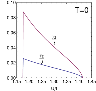
Figure 1: (Color online) Pairing interaction $\gamma_{2}$ normalized to the hopping parameter $t$ (upper curve) and the antiferromagnetic-exchange parameter $J=4t^{2}/U$ (lower curve) as a function of the Coulomb interaction $U/t$ calculated at zero temperature and half filling $\bar{\mu}=0$ for the two-dimensional Hubbard model with nearest-neighbors hopping.

are given in terms of the $CP^{1}$ normal $(g)$ and anomalous $(f)$ correlation functions

$$g({\bf r-r^{\prime}})=-\left\langle\zeta_{\alpha}({\bf{r}}\tau)\bar{\zeta}_{\alpha}({\bf{r}^{\prime}}\tau)\right\rangle_{\text{SU(2)}},\$$

$$f({\bf r-r^{\prime}})=\left\langle\zeta_{\alpha}({\bf{r}}\tau)\zeta_{\alpha}({\bf{r}}^{\prime}\tau)\right\rangle_{\text{SU(2)}}$$ (80)

which can be readily evaluated using the propagator of the $\zeta$ fields in Eq.(56).

V Hamiltonian with pairing term

From the result in Eq.(77) we can deduce the spin-singlet pairing possibility in the fermionicsector. To bring the kinetic-energy term to a standard form, one performs a rotation of the fermionic variables on one of the sublattices in a manner similar to the bosonic transformation in Eq.(48).

$$h_{\uparrow}({\bf{r}}^{\prime}\tau)\rightarrow-h_{\downarrow}({\bf{r}}^{\prime}\tau),$$

$$h_{\downarrow}({\bf{r}}^{\prime}\tau)\rightarrow h_{\uparrow}({\bf{r}}^{\prime}\tau).\ \$$ (81)

As a result the hopping term assumes the conventional form that is diagonal in the spin indices

$$S^{(1)}_{t}[\bar{h},h]=-\tilde{t}\sum_{\left\langle\bf{r}\bf{r}^{\prime}\right\rangle,\alpha}\int_{0}^{\beta}\bar{h}_{\alpha}(\textbf{r}\tau)h_{\alpha}(\textbf{r}^{\prime}\tau),$$ (82)

while the second-order term is given by

$$S^{(2)}[\bar{h},h]=\sum_{\left\langle{\bf{r}}{\bf{r}}^{\prime}\right\rangle}\int^{\beta}_{0}d{\tau}\left[\gamma_{1}n({\bf{r}}\tau)n({\bf{r}}^{\prime}\tau)\right.$$

$$\left.-\gamma_{2}\bar{\cal A}_{h}({\bf{r}}\tau{\bf{r}}^{\prime}\tau){{\cal A}_{h}}({\bf{r}}\tau{\bf{r}}^{\prime}\tau)\right],$$ (83)

where

$${\cal A}_{h}({\bf{r}}\tau{\bf{r}}^{\prime}\tau)=\frac{h_{\uparrow}({\bf{r}}\tau)h_{\downarrow}({\bf{r}}^{\prime}\tau)-h_{\downarrow}({\bf{r}}\tau)h_{\uparrow}({\bf{r}}^{\prime}\tau)}{\sqrt{2}},$$

$$\bar{\cal A}_{h}({\bf{r}}\tau{\bf{r}}^{\prime}\tau)=\frac{\bar{h}_{\downarrow}({\bf{r}}^{\prime}\tau)\bar{h}_{\uparrow}({\bf{r}}\tau)-\bar{h}_{\uparrow}({\bf{r}}^{\prime}\tau)\bar{h}_{\downarrow}({\bf{r}}\tau)}{\sqrt{2}}$$ (84)

are the bond operators relevant for a singlet pairing. The rotational invariance of the right-hand side in Eq.(83) is manifest since

$$-\bar{\cal A}_{h}({\bf r}\tau{\bf r}^{\prime}\tau){\cal A}_{h}({\bf r}\tau{\bf r}^{\prime}\tau)=$$

$${\bf S}_{h}({\bf r}\tau)\cdot{\bf S}_{h}({\bf r^{\prime}}\tau)-\frac{1}{4}n_{h}({\bf r}\tau)n_{h}({\bf r^{\prime}}\tau).$$ (85)

The coefficients $\gamma_{1}$ and $\gamma_{2}$ are given by Eq.(79). By noting that $g({\bf d})=0$ and $f({\bf 0})=0$ one obtains

$$\gamma_{1}=\frac{4t^{2}}{U}\left[f^{2}({\bf d})+\frac{1}{2}g^{2}({\bf 0})\right],$$

$$\gamma_{2}=\frac{4t^{2}}{U}\left[3f^{2}({\bf d})\right]=J\left[\frac{3Q^{2}}{J^{2}(\Delta)}\right],$$ (86)

where the $f,g$-correlation functions can be computed with the help of the $CP^{1}$ propagators: see Eq.(57). The effective nonretarded interaction containing $\gamma_{2}$ in front of the $\bar{\cal A}({\bf r}\tau{\bf r}^{\prime}\tau){\cal A}({\bf r}\tau{\bf r}^{\prime}\tau)$ term is negative and therefore constitutes the attractive potential for fermion pairing. We can see that the coefficient $\gamma_{2}$ is not just given by the bare AF exchange $J=4t^{2}/U$ but is renormalized downward by the quantity $Q$ that is related to the antifferomagnetic spin stiffness as delineated in Sec.IVD dealing with the SU(2) spin sector. We have calculated $Q$ self-consistently using Eq.(58). The result is plotted in Fig.1. Note that the pairing interaction survives in rather narrow range of the Coulomb interaction $1.17<U/t<1.41$. This result suggests that superconductivity in the Hubbard model, if possible, represents a rather delicate balance between kinetic energy and Coulomb interaction. In this context, we note that the deleterious effects of the Coulomb interaction superconductivity in cuprates have been largely ignored in the literature. Furthermore, since $\gamma_{1}>0$ in the density-density term in Eq.(83), many sorts of the charge-ordered states can be stabilized, including e.g., charge-density wave states, which in general compete with superconductivity. This is in contrast to the BCS theory where the only instability of a Fermi liquid is the Cooper instability: the superconducting order is generic.

VI CONCLUSIONS and perspectives

The basic physics of strongly correlated electronic systems is the competition between the two tendencies of the electron to spread out as a wave and to localize as a particle combined with magnetism. That is, the interplay of the spin and the charge degree of freedom is the central issue. While there is a growing consensus that superconductivity in the cuprates arises from strong short-range Coulomb interactions between electrons rather than the traditional electron-phonon interaction, the precise nature of the pairing interaction remains controversial. While the principal focus of the present work is theoretical, the choice of model and the approach is motivated in the experimentally observed properties of cuprates. Therefore, in the present work we hope to shed some light on this controversial issue with the purpose to understand better the physical properties of most common model for cuprates. To this end, we have discussed in the present work the Hubbard model in the spin-rotational invariant formulation which observes the important symmetries involved. We presented a field-theoretic description of a microscopic model that reveals an intimate relationship between the spin-SU(2) and charge-U(1) symmetry and pairings. We found that the maximal strength of the effective pairing interaction parameter is observed in a rather narrow range of $U/t$ with the kinetic energy comparable to the Coulomb interaction. Moreover, the form of the effective fermionic action suggests that other competing ordered phases can occur simultaneously, which can quench the superconductivity substantially. Therefore, the issue of pairing interaction is not settling the question about the long-range superconducting order in the Hubbard model. As far as modeling of cuprates is concerned there is also a problem of interplane interaction, entirely omited in the present work, which can affect the bulk superconductivity considerably. In closing we note that the pairing interaction itself cannot be measured directly: one needs to analyze key experiments which reveal fingerprints of it. Thus, the continuing experimental search for a pairing glue in the cuprates is important and will play an essential role in determining the origin of the high-$T_{c}$ pairing interaction.

VII ACKNOWLEDGMENTS

One of us (V.A.A.) acknowledges the financial support from the International Max Planck Research School “Dynamical Processes in Atoms, Molecules, and Solids”, T.K.K was supported by the Ministry of Education and Science MEN under Grant No. 1PO3B 103 30 in the years 2006-2008. We are grateful to T. A. Zaleski for numerical evaluation and plotting of the data for Fig.1.

VIII APPENDIX A:U(1) PHASE AVERAGES

In this section we evaluate the expression for U(1) phase propagator. Two point phase-phase propagator for the Bosonic phase variables is defined as

$$g_{z}({\bf{r}}\tau{\bf{r}}^{\prime}\tau^{\prime})=\left\langle\bar{z}({\bf{r}}\tau)z({\bf{r}}^{\prime}\tau^{\prime})\right\rangle.$$ (87)

The averaging in this definition is over the U(1) phase field and

$$\left\langle...\right\rangle=\frac{\int{D\phi}...e^{-S_{0}[\phi]}}{\int{D\phi}e^{-S_{0}[\phi]}}.$$ (88)

Here the complex variables $z({\bf{r}}\tau)$ are defined as $z({\bf{r}}\tau)=e^{i\phi({\bf{r}}\tau)}$. The variables $\phi({\bf{r}}\tau)$ satisfy the following boundary conditions:

$$\phi({\bf r}\beta)-\phi({\bf r}0)=2{\pi}m({{\bf r}}).$$ (89)

It is very convenient to satisfy the boundary conditions by decomposing the phase field in terms of a periodic field $\phi({\bf{r}}\tau)$ and a term linear in $\tau$. We set

$$\phi({\bf r}\tau)=\tilde{\phi}({\bf r}\tau)+\frac{2\pi\tau}{\beta}m({\bf r})$$ (90)

with $\tilde{\phi}(\beta)=\tilde{\phi}(0)$. Summing over the phase field $\varphi$ means to integrate all $\phi({\bf{r}}\tau)$ configurations and perform the summation over the integers $n$. Then we write the phase variables $\phi({\bf{r}}\tau)$ in the Fourier-transformed form

$$\tilde{\phi}({\bf{r}}\tau)=\frac{\phi_{0}({\bf{r}})}{\beta}+\frac{1}{\beta}\sum^{\infty}_{n=1}\left[\phi_{n}({\bf{r}})e^{i\omega_{n}\tau}+\phi^{\ast}({\bf{r}})e^{-i\omega_{n}\tau}\right].$$ (91)

The weight of the averaging in the expression of the phase correlator is given by the following exponential:

$$e^{-S_{0}[\phi]}=e^{-\sum_{{\bf{r}}}\int^{\beta}_{0}d\tau{\dot{\phi}^{2}({\bf{r}}\tau)}/{U}\dot{\phi}}e^{-S_{0}[m]},$$ (92)

where the action $S_{0}[m]$ is the topological part of the action and is given by

$$S_{0}[\phi] = \frac{2}{\beta{U}}\sum_{{\bf{r}}}\sum_{n}|\phi_{n}({\bf{r}})|^{2},$$

$$S_{0}[m] = \sum_{{\bf{r}}}\left[\frac{4\pi^{2}m^{2}({\bf r})}{\beta{U}}-\frac{4\pi{i}\mu}{U}m({\bf r})\right].$$ (93)

Now we evaluate the average. We write first the nontopological part of the action

$$g_{z}({\bf{r}}\tau{\bf{r}}^{\prime}\tau^{\prime}) = \frac{\int[{\cal{D}}\phi]e^{-i\phi({\bf{r}}\tau)}e^{i\phi({\bf{r}}\tau)}e^{-{2}/{\beta{U}}\sum_{{\bf{r}}}\sum_{n}|\phi_{n}({\bf{r}}\tau)|^{2}}}{\int[{\cal{D}}\phi]e^{-{2}/{\beta{U}}\sum_{{\bf{r}}}\sum_{n}|\phi_{n}({\bf{r}})|^{2}}}$$ (94)

$$=\delta_{\bf rr^{\prime}}\frac{\prod^{\infty}_{n=1}\left[\frac{U\beta}{4\omega^{2}_{n}}\right]e^{-{U}/{2\beta}\sum^{\infty}_{n=1}{1}/{\omega^{2}_{n}}\left\{\left[\sin(\omega_{n}\tau)\sin(\omega_{n}\tau^{\prime})\right]^{2}+\left[\cos(\omega_{n}\tau)-\cos(\omega_{n}\tau^{\prime})\right]^{2}\right\}}}{\prod^{\infty}_{n=1}\left[\frac{U\beta}{4\omega^{2}_{n}}\right]}$$

By using the identity

$$\left[\sin(x)-\sin(y)\right]^{2}+\left[\cos(x)-\cos(y)\right]^{2}$$

$$=2-2[\cos(x)\cos(y)+\sin(x)\sin(y)]$$

$$=2-2\cos(x-y)$$ (95)

one obtains

$$g_{z}({\bf{r}}\tau{\bf{r}}^{\prime}\tau^{\prime})=\delta_{\bf rr^{\prime}}e^{-{U}/{\beta}\sum^{\infty}_{n=1}{1}/{\omega^{2}_{n}}\left\{1-\cos\left[\omega_{n}(\tau-\tau^{\prime})\right]\right\}}.$$ (96)

Now, in order to calculate the sum in the exponential we use the following identity:

$$|x|-\frac{x^{2}}{\beta}=\sum^{\infty}_{n=1}\left(\frac{4}{\beta\omega^{2}_{n}}-\frac{4\cos(\omega_{n}\tau)x}{\beta\omega^{2}_{n}}\right),$$ (97)

where $-\beta\leq x\leq\beta$. And finally we get

$$g_{z}({\bf{r}}\tau{\bf{r}}^{\prime}\tau^{\prime})=\delta_{\bf rr^{\prime}}e^{-{U}/{4}\left[|\tau-\tau^{\prime}|-{(\tau-\tau^{\prime})^{2}}/{\beta}\right]}$$ (98)

Now we are ready to calculate the four-point phase correlator:

$$\left\langle\bar{z}({\bf{r}}_{1}\tau)z({\bf{r}}^{\prime}_{1})\bar{z}({\bf{r}}_{2}\tau^{\prime})z({\bf{r}}_{2}\tau^{\prime})\right\rangle_{\text{U(1)}}=$$

$$\left\langle\bar{z}({\bf{r}}_{1}\tau)z({\bf{r}}^{\prime}_{1})\right\rangle_{\text{U(1)}}\left\langle\bar{z}({\bf{r}}_{2}\tau^{\prime})z({\bf{r}}_{2}\tau^{\prime})\right\rangle_{\text{U(1)}}+$$

$$+\left\langle\bar{z}({\bf{r}}_{1}\tau)z({\bf{r}}^{\prime}_{2}\tau^{\prime})\right\rangle_{\text{U(1)}}\left\langle z({\bf{r}}^{\prime}_{1}\tau)\bar{z}({\bf{r}}_{2}\tau^{\prime})\right\rangle_{\text{U(1)}}$$ (99)

By using the result in Eq. (98) we get Eq.(36).

IX APPENDIX B:SU(2) AVERAGE

The composition formula for the rotational matrices in the angular representation is given by

$$R^{{\dagger}}({\bf r}\tau)R({\acute{\bf r}}\tau)=\frac{1}{\sqrt{2}}\left[\begin{array}[]{cc}\sqrt{1+{\bf{\Omega}}(\textbf{r}\tau){\bf{\Omega}}(\textbf{r}^{\prime}\tau)}\exp(\frac{i}{2}\Phi)&\sqrt{1-{\bf{\Omega}}(\textbf{r}\tau){\bf{\Omega}}(\textbf{r}^{\prime}\tau)}\exp(\frac{i}{2}\bar{\Phi})\\ -\sqrt{1-{\bf{\Omega}}(\textbf{r}\tau){\bf{\Omega}}(\textbf{r}^{\prime}\tau)}\exp(-\frac{i}{2}\bar{\Phi})&\sqrt{1+{\bf{\Omega}}(\textbf{r}\tau){\bf{\Omega}}(\textbf{r}^{\prime}\tau)}\exp(-\frac{i}{2}\Phi)\end{array}\right],$$ (102)

where $\Phi\equiv\Phi[{\bf\Omega}({\bf r}\tau),{\bf\Omega}({\bf r^{\prime}}\tau),{\bf z}]$ is the signed solid angle spanned by the vectors ${\bf\Omega}({\bf r}\tau),{\bf\Omega}({\bf r^{\prime}}\tau)$ and z with $\bar{\Phi}=\Phi[{\bf\Omega}({\bf r}\tau),-{\bf\Omega}({\bf r^{\prime}}\tau)]-2\varphi({\bf r}\tau)$. In the complex projective representation, Eq.(102) reads

$$R^{{\dagger}}({\bf r}\tau)R({\acute{\bf r}}\tau)=\left[\begin{array}[]{cc}{\bar{\zeta}}_{1}(\textbf{r}\tau)\zeta_{1}(\textbf{r}^{\prime}\tau)+{\bar{\zeta}}_{2}(\textbf{r}\tau)\zeta_{2}(\textbf{r}^{\prime}\tau)&-{\bar{\zeta}}_{1}(\textbf{r}\tau)\bar{\zeta}_{2}(\textbf{r}^{\prime}\tau)+{\bar{\zeta}}_{2}(\bf{r}\tau)\bar{\zeta}_{1}(\textbf{r}^{\prime}\tau)\\ -{\zeta}_{2}(\textbf{r}\tau)\zeta_{1}(\textbf{r}^{\prime}\tau)+{\zeta}_{1}(\textbf{r}\tau)\zeta_{2}(\textbf{r}^{\prime})&{\zeta}_{2}(\textbf{r}\tau)\bar{\zeta}_{2}(\textbf{r}^{\prime}\tau)+{\zeta}_{1}(\textbf{r}\tau)\bar{\zeta}_{1}(\textbf{r}^{\prime}\tau)\end{array}\right].\$$ (105)

The form of Eq.(105) suggests the use of the bond operators defined by Eqs.(47) and (71), so that the product of rotational matrices can be written in a compact form

$$R^{{\dagger}}({\bf r}\tau)R({\acute{\bf r}}\tau)=\left[\begin{array}[]{cc}{\cal F}&-\bar{\cal A}\\ {\cal A}&\bar{\cal F}\end{array}\right]({\bf{r}}\tau{\bf{r}}^{\prime}\tau)$$ (108)

$$R^{{\dagger}}({\acute{\bf r}}\tau{\bf r}\tau)R({\bf r}\tau)=\left[\begin{array}[]{cc}\bar{\cal F}&\bar{\cal A}\\ -{\cal A}&{\cal F}\end{array}\right]({\bf{r}}\tau{\bf{r}}^{\prime}\tau).$$ (111)

With the help of the above equation it is easy to write down the components of the $M$ matrix

Under the transformation the bond operators become

$${\cal{F}}({\bf{r}}\tau{\bf{r}}^{\prime}\tau) \to {\cal{F}^{\prime}}({\bf{r}}\tau{\bf{r}}^{\prime}\tau)$$

$$= \frac{-\bar{\zeta}_{1}({\bf{r}}\tau){\zeta}_{2}({\bf{r}}^{\prime}\tau)+\bar{\zeta}_{2}({\bf{r}}\tau){\zeta}_{1}({\bf{r}}^{\prime}\tau)}{\sqrt{2}}$$

$${\cal{A}}({\bf{r}}\tau{\bf{r}}^{\prime}\tau) \to {\cal{A}^{\prime}}({\bf{r}}\tau{\bf{r}}^{\prime}\tau)$$ (112)

$$= \frac{{\zeta}_{1}({\bf{r}}\tau){\zeta}({\bf{r}}^{\prime}\tau)+{\zeta}_{2}({\bf{r}}\tau){\zeta}_{2}({\bf{r}}^{\prime}\tau)}{\sqrt{2}}.$$

$$M_{12;21}({\bf{r}}\tau,{\bf{r}}^{\prime}\tau|{\bf{r}}^{\prime}\tau,{\bf{r}}\tau)=\left\langle\left[R^{{\dagger}}({\bf{r}}\tau)R({\bf{r}}^{\prime}\tau)\right]_{12}\left[R^{{\dagger}}({\bf{r}}^{\prime}\tau)R({\bf{r}}\tau)\right]_{21}\right\rangle_{\text{SU(2})}$$

$$=\langle\bar{\cal{A}^{\prime}}({\bf{r}}\tau{\bf{r}}^{\prime}\tau){\cal{A}^{\prime}}({\bf{r}}\tau{\bf{r}}^{\prime}\tau)\rangle_{\text{SU(2)}}=\left\langle\left[\bar{\zeta}_{1}({\bf{r}}^{\prime}\tau)\bar{\zeta}_{1}({\bf{r}}\tau)+\bar{\zeta}_{2}({\bf{r}}^{\prime}\tau)\bar{\zeta}_{2}({\bf{r}}\tau)\right]\left[{\zeta}_{1}({\bf{r}}\tau)\zeta_{1}({\bf{r}}^{\prime})+\zeta_{2}({\bf{r}}\tau)\zeta_{2}({\bf{r}}^{\prime}\tau)\right]\right\rangle_{\text{SU(2)}}$$

$$=\left\langle\sum_{\alpha,\beta}\bar{\zeta}_{\alpha}({\bf{r}}^{\prime}\tau)\bar{\zeta}_{\alpha}({\bf{r}}\tau){\zeta}_{\beta}({\bf{r}}\tau){\zeta}_{\beta}({\bf{r}}^{\prime}\tau)\right\rangle_{\text{SU(2)}}.$$ (113)

Furthermore, by implementing the Wick theorem to the $CP^{1}$ averages

$$\left\langle\bar{\zeta}_{\alpha}({\bf{r}}^{\prime}\tau)\bar{\zeta}_{\alpha}({\bf{r}}\tau){\zeta}_{\beta}({\bf{r}}\tau){\zeta}_{\beta}({\bf{r}}^{\prime}\tau)\right\rangle_{\text{SU(2)}} = \left\langle\bar{\zeta}_{\alpha}({\bf{r}}^{\prime}\tau)\bar{\zeta}_{\alpha}({\bf{r}}\tau)\right\rangle_{\text{SU(2)}}\left\langle{\zeta}_{\beta}({\bf{r}}\tau){\zeta}_{\beta}({\bf{r}}^{\prime}\tau)\right\rangle_{\text{SU(2)}}$$ (114)

$$+ \left\langle\bar{\zeta}_{\alpha}({\bf{r}}^{\prime}\tau)\zeta_{\beta}({\bf{r}}\tau)\right\rangle_{\text{SU(2)}}\left\langle\bar{\zeta}_{\alpha}({\bf{r}}\tau)\zeta_{\beta}({\bf{r}}^{\prime}\tau)\right\rangle_{\text{SU(2)}}$$

$$+ \left\langle\bar{\zeta}_{\alpha}({\bf{r}}^{\prime}\tau)\zeta_{\beta}({\bf{r}}^{\prime}\tau)\right\rangle_{\text{SU(2)}}\left\langle\bar{\zeta}_{\alpha}({\bf{r}}\tau)\zeta_{\beta}({\bf{r}}\tau)\right\rangle_{\text{SU(2)}}$$

$$= \delta_{\alpha\alpha}\delta_{\beta\beta}f(-{\bf d})f({\bf d})+\delta_{\alpha\beta}\delta_{\beta\alpha}g({\bf d})g(-{\bf d})+\delta_{\alpha\beta}\delta_{\beta\alpha}g({\bf 0})g({\bf 0})$$

In a similar manner

$$M_{11,11}({\bf{r}}\tau,{\bf{r}}^{\prime}\tau|{\bf{r}}^{\prime}\tau,{\bf{r}}\tau)=2\left[g^{2}({\bf 0})-f^{2}({\bf d})\right],$$

$$M_{11;22}({\bf{r}}\tau,{\bf{r}}^{\prime}\tau|{\bf{r}}^{\prime}\tau,{\bf{r}}\tau)=2\left[f^{2}({\bf 0})-g^{2}({\bf d})\right],$$

$$M_{12;21}({\bf{r}}\tau,{\bf{r}}^{\prime}\tau|{\bf{r}}^{\prime}\tau,{\bf{r}}\tau)=4f^{2}({\bf d})+2g({\bf d})+2g({\bf 0}),$$

$$M_{12;12}({\bf{r}}\tau,{\bf{r}}^{\prime}\tau|{\bf{r}}^{\prime}\tau,{\bf{r}}\tau)=-\left[6f^{2}({\bf d})+2f^{2}({\bf 0})\right],$$ (115)

where we have used that $f(-{\bf d})=f({\bf d})$ and $g(-{\bf d})=g({\bf d})$. It is not difficult to see that

$$M_{11,11}({\bf{r}}\tau,{\bf{r}}^{\prime}\tau|{\bf{r}}^{\prime}\tau,{\bf{r}}\tau)=M_{22,22}({\bf{r}}\tau,{\bf{r}}^{\prime}\tau|{\bf{r}}^{\prime}\tau,{\bf{r}}\tau),$$

$$M_{11;22}({\bf{r}}\tau,{\bf{r}}^{\prime}\tau|{\bf{r}}^{\prime}\tau,{\bf{r}}\tau)=M_{22,11}({\bf{r}}\tau,{\bf{r}}^{\prime}\tau|{\bf{r}}^{\prime}\tau,{\bf{r}}\tau),$$

$$M_{12;21}({\bf{r}}\tau,{\bf{r}}^{\prime}\tau|{\bf{r}}^{\prime}\tau,{\bf{r}}\tau)=M_{21;12}({\bf{r}}\tau,{\bf{r}}^{\prime}\tau|{\bf{r}}^{\prime}\tau,{\bf{r}}\tau),$$

$$M_{12;12}({\bf{r}}\tau,{\bf{r}}^{\prime}\tau|{\bf{r}}^{\prime}\tau,{\bf{r}}\tau)=M_{21;21}({\bf{r}}\tau,{\bf{r}}^{\prime}\tau|{\bf{r}}^{\prime}\tau,{\bf{r}}\tau),$$ (116)

while all the remaining components of the $M$ matrix vanish.

X APPENDIX C:USEFUL OPERATOR IDENTITIES

By introducing the fermionic representation of the $1/2$-spin operators

$${\bf{S}}_{h}({\bf{r}}\tau)=\frac{1}{2}\sum_{\alpha\beta}\bar{h}_{\alpha}({\bf{r}}\tau)\hat{\sigma}_{\alpha\beta}h_{\beta}({\bf{r}}\tau)$$ (117)

and the following bond operators:

$${\cal A}_{h}^{\prime}({\bf{r}}\tau{\bf{r}}^{\prime}\tau)=\frac{h_{\uparrow}({\bf{r}}\tau)h_{\uparrow}({\bf{r}}^{\prime}\tau)+h_{\downarrow}({\bf{r}}\tau)h_{\downarrow}({\bf{r}}^{\prime}\tau)}{\sqrt{2}},$$

$${\cal A}_{h}({\bf{r}}\tau{\bf{r}}^{\prime}\tau)=\frac{h_{\uparrow}({\bf{r}}\tau)h_{\downarrow}({\bf{r}}^{\prime}\tau)-h_{\downarrow}({\bf{r}}\tau)h_{\uparrow}({\bf{r}}^{\prime}\tau)}{\sqrt{2}},$$

$${\cal F}_{h}({\bf{r}}\tau{\bf{r}}^{\prime}\tau)=\frac{\bar{h}_{\uparrow}({\bf{r}}\tau)h_{\uparrow}({\bf{r}}^{\prime}\tau)+\bar{h}_{\downarrow}({\bf{r}}\tau)h_{\downarrow}({\bf{r}}^{\prime}\tau)}{\sqrt{2}},$$ (118)

one can prove the following useful identities that involve four-fermion products that appear in the second-order cumulant expansion. For the spin and charge products, we have

$${\bf{S}}_{h}({\bf{r}}\tau)\cdot{\bf{S}}_{h}({\bf{r}}^{\prime}\tau)=\frac{n_{h}({\bf{r}}^{\prime}\tau)}{4}$$

$$-\frac{\bar{\cal A}_{h}({\bf{r}}\tau{\bf{r}}^{\prime}\tau){\cal A}_{h}({\bf{r}}\tau{\bf{r}}^{\prime}\tau)}{2}-\frac{\bar{\cal F}_{h}({\bf{r}}\tau{\bf{r}}^{\prime}\tau){\cal F}_{h}({\bf{r}}\tau{\bf{r}}^{\prime}\tau)}{2},$$

$$\frac{n_{h}({\bf{r}}\tau)n_{h}({\bf{r}}^{\prime}\tau)}{2}=\frac{n_{h}({\bf{r}}^{\prime}\tau)}{2}$$

$$+\bar{\cal A}_{h}({\bf{r}}\tau{\bf{r}}^{\prime}\tau){\cal A}_{h}({\bf{r}}\tau{\bf{r}}^{\prime}\tau)-\bar{\cal F}_{h}({\bf{r}}\tau{\bf{r}}^{\prime}\tau){\cal F}_{h}({\bf{r}}\tau{\bf{r}}^{\prime}\tau).$$ (119)

Furthermore, for the prpducts of fermionic variables that appear in the calculation of the $M$ matrix, one finds

$$\sum_{\alpha\beta}\bar{h}_{\alpha}({\bf{r}}\tau)h_{\alpha}({\bf{r}}^{\prime}\tau)\bar{h}_{\beta}({\bf{r}}^{\prime}\tau)h_{\beta}({\bf{r}}\tau)=n_{h}({\bf{r}}\tau)$$

$$-\frac{n_{h}({\bf{r}}\tau)n_{h}({\bf{r}}^{\prime}\tau)}{2}-2{\bf{S}}_{h}({\bf{r}}\tau)\cdot{\bf{S}}_{h}({\bf{r}}^{\prime}\tau),$$

$$\sum_{\alpha\beta}\bar{h}_{\alpha}({\bf{r}}\tau)h_{\beta}({\bf{r}}^{\prime}\tau)\bar{h}_{\beta}({\bf{r}}^{\prime}\tau)h_{\alpha}({\bf{r}}\tau)=2n_{h}({\bf{r}}\tau)$$

$$-n_{h}({\bf{r}}\tau)n_{h}({\bf{r}}^{\prime}\tau),$$

$$\sum_{\alpha\beta}\bar{h}_{\alpha}({\bf{r}}\tau)h_{\beta}({\bf{r}}^{\prime}\tau)\bar{h}_{\alpha}({\bf{r}}^{\prime}\tau)h_{\beta}({\bf{r}}\tau)=n_{h}({\bf{r}}\tau)$$

$$-2\bar{\cal A}_{h}^{\prime}({\bf{r}}\tau{\bf{r}}^{\prime}\tau){\cal A}_{h}^{\prime}({\bf{r}}\tau{\bf{r}}^{\prime}\tau),$$ (120)

where, by simple inspection, one can find that the spin-rotational symmetry is apparent.

References

- (1) J. Bardeen, L. N. Cooper, and J. R. Schrieffer, Phys. Rev. 108,1175 (1957).
- (2) J. G. Bednorz and K. A. Müller, Z. Phys. B: Condens. Matter 64, 189 (1986).
- (3) P. W. Anderson, Science 317, 1705 (2007).
- (4) J. E. Hirsch, Phys. Rev. B 31, 4403 (1985).
- (5) N. Furukawa and M. Imada, J. Phys. Soc. Jpn. 61, 3331 (1992).
- (6) G. Fano, F. Ortolani, and A. Parola, Phys. Rev. B 42, 6877 (1990).
- (7) E. Dagotto, A. Moreo, F. Ortolani, D. Poilblanc, and J. Riera, Phys. Rev. B 45, 10741 (1992).
- (8) T. Kashima and M. Imada, J. Phys. Soc. Jpn. 70, 2287 (2001).
- (9) D. Rohe and W. Metzner, Phys. Rev. B 71, 115116 (2005).
- (10) T. Maier, M. Jarrell, T. Pruschke, and M. H. Hettler, Rev. Mod. Phys. 77 1027 (2005).
- (11) T. A. Maier, M. S. Jarrell, and D. J. Scalapino, Phys. Rev. Lett., 96, 047005 (2006).
- (12) T. A. Maier, M. Jarrell, and D . J. Scalapino, Phys.Rev.B, 74, 094513 (2006).
- (13) P. Monthoux and D. J. Scalapino, Phys. Rev. Lett., 72, 1874 (1994).
- (14) A. Moreo and D. J. Scalapino, Phys. Rev. B, 43, 8211 (1991).
- (15) F. C. Zhang and T. M. Rice, Phys. Rev. B 37, R3759 (1988). Rev. Mod. Phys. 77, 1027 (2005); A. M. S. Tremblay, B. Kyung, and D. Senechal, J. Low Temp. Physics 32, 424 (2006).
- (16) J. Zaanen, G. A. Sawatzky, and J. W. Allen, Phys. Rev. Lett. 55, 418 (1985).
- (17) R. B. Laughlin, cond-mat/0209269 (unpublished).
- (18) T. K. Kopeć, Phys. Rev. B 73, 132512 (2006).
- (19) T. A. Zaleski, T. K. Kopeć, Phys. Rev. B 77, 125120 (2008).
- (20) See for instance J.W. Negele and H. Orland, Quantum Many Particle Systems, Frontiers in Physics (Addison-Wesley), (1988).
- (21) H. J. Schulz, Phys. Rev. Lett. 65, 2462 (1990).
- (22) A. Auerbach, Interacting Electrons and Quantum Magnetism (Springer-Verlag, New York, 1994).
- (23) It is evident that the retardation plays a crucial role in the BCS mechanism. In the typical metallic superconductor, the Fermi energy is of the order of several eV while phonon frequencies are of the order eV, therefore . Since the renormalization of the Coulomb pseudopotential is logarithmic, this large value of the retardation is required. In the cuprate superconductors, on the other hand, , where is the superconducting gap, so the “HTSC” materials are clearly in the nonretarded regime.