Structural and spectral properties of a family of deterministic recursive trees: Rigorous solutions

Abstract

As one of the most significant models, the uniform recursive tree (URT) has found many applications in a variety of fields. In this paper, we study rigorously the structural features and spectral properties of the adjacency matrix for a family of deterministic uniform recursive trees (DURTs) that are deterministic versions of URT. Firstly, from the perspective of complex networks, we investigate analytically the main structural characteristics of DURTs, and obtain the accurate solutions for these properties, which include degree distribution, average path length, distribution of node betweenness, and degree correlations. Then we determine the complete eigenvalues and their corresponding eigenvectors of the adjacency matrix for DURTs. Our research may shed light in better understanding of the features for URT. Also, the analytical methods used here is capable of extending to many other deterministic networks, making the precise computation of their properties (especially the full spectrum characteristics) possible.

1 Introduction

Structural characterization is very significant for the study in the field of complex networks that have become a focus of attention for the scientific community [1, 2, 3]. In the past decade, great efforts have been dedicated to characterizing and understanding the structural properties of real networks [4], including degree distribution, average path length (APL), betweenness, degree correlations, fractality, and so forth. These measures have a profound effect on various dynamical processes taking place on top of complex networks [5], such as robustness [6, 7, 8, 9], epidemic spreading [10, 11], synchronization [12, 13, 14, 15], and games [16].

The foregoing measurements focus on direct measurements of structural properties of networks, and play an important role in understanding network complexity [17]. Aside from these measurements there exists a vast literature related to spectrum of complex networks [18, 19, 20, 21], which provides useful insight into the relevant structural properties of and dynamical processes on graphs. In contrast to the fact that structural features capture the static topological properties of complex networks, spectra (eigenvalues and eigenvectors) of adjacency matrix provide global measures of the characterization for network topology. In a variety of dynamical processes, the impact of network structure is encoded in the spectra of its adjacency matrix, especially the extreme eigenvalues and their corresponding eigenvectors. For example, in the dynamical model for the spreading of infections, the epidemic thresholds are governed by the largest eigenvalue of the adjacency matrix [22, 23], which also plays a fundamental role in determining critical couplings for the onset of coherent behavior [24]. In addition, recent research showed that in the Susceptible-Infected model of epidemic outbreaks on complex networks, the eigenvector corresponding to the largest eigenvalue are related to spreading power of network nodes [25]. In spite of the importance of the eigenvalues and eigenvectors of the adjacency matrix, however, until now, most analysis of the spectra has been confined to approximate or numerical methods, the latter of which is prohibitively time and memory consuming for large-scale networks [18].

On the other hand, in order to mimic real systems and study their structural properties, a great number of network models have been presented [1, 2, 3], among which the uniform recursive tree (URT) is perhaps one of the most widely studied models [26]. It is now established that the URT, together with the famous Erdös-Rényi model [27], constitutes the two principal models [28, 29] of random graphs. As one of the simplest trees, the URT is constructed as follows: start with a single node, at each time step, we attach a new node to an existing node selected at random. It has found many important applications in various areas. For example, it has been suggested as models for the spread of epidemics [30], the family trees of preserved copies of ancient or medieval texts [31], chain letter and pyramid schemes [32], to name but a few.

Recently, a class of deterministically growing tree-like networks have been proposed to describe real-world systems whose number of nodes increases exponentially with time [33]. We call them deterministic uniform recursive trees (DURTs), since they are deterministic versions of URT. This kind of deterministic models have received considerable attention from the scientific communities and have turned out to be a useful tool [34, 35, 36, 37, 38, 39, 40, 41, 42, 43, 44, 45, 46, 47, 48, 49, 50, 51]. Although uniform recursive tree is well understood [26, 28, 29, 30, 31, 52, 53], relatively less is known about the structural and other nature of the DURTs [33].

In this paper, from the viewpoint of complex networks, we offer a comprehensive analysis of the deterministic uniform recursive trees (DURTs) [33]. We firstly determine exactly relevant structural properties of the DURTs, including degree distribution, average path length, betweenness distribution, and degree correlations. Then, using methods of graph theory and algebra, We calculate all the eigenvalues and eigenvectors of the adjacency matrix, which are obtained through the recurrence relations derived from the very structure of the DURTs.

2 The deterministic uniform recursive trees

The deterministic uniform recursive trees under consideration are constructed in an iterative way [33]. We denote the trees (networks) after $t$ steps by $U_{t}$ ($t\geq 0$). Then the networks are built as follows. For $t=0$, $U_{0}$ is an edge connecting two nodes. For $t\geq 1$, $U_{t}$ is obtained from $U_{t-1}$. We attach $m$ new nodes to each node in $U_{t-1}$. This iterative process is repeated, then we obtain a class of deterministically growing trees with an exponential decreasing spectrum of degrees as shown below. The definition of the model for a particular case of $m=1$ is illustrated schematically in figure 1.

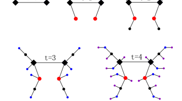
Figure 1: Illustration of a deterministic uniform recursive tree for the special case of $m=1$, showing the first several steps of growth process.

We first compute the total number of nodes $N_{t}$ and the total number of edges $E_{t}$ in the $U_{t}$. Let $n_{v}(t)$ and $n_{e}(t)$ denote the numbers of nodes and edges created at step $t$, respectively. Then, $n_{v}(0)=N_{0}=2$ and $n_{e}(0)=1$. By construction, we have $n_{v}(t)=m\,N_{t-1}$, thus $N_{t}=n_{v}(t)+N_{t-1}=(1+m)\,N_{t-1}$. Considering the initial condition $N_{0}=2$, we obtain $N_{t}=2\,(1+m)^{t}$ and $n_{v}(t)=2\,m\,(1+m)^{t-1}$. Thus, $E_{t}=N_{t}-1=2\,(1+m)^{t}-1$. Notice that at arbitrary step $t\geq 1$, the addition of each new node leads to only new edge, so $n_{e}(t)=n_{v}(t)=2\,m\,(1+m)^{t-1}$ for all $t\geq 1$.

3 Structural properties

In this section, we investigate four important structural properties of $U_{t}$, including degree distribution, average path length, betweenness distribution, and degree correlations.

3.1 Degree distribution

By definition, the degree of a node $i$ is the number of edges connected to $i$. The degree distribution $P(k)$ of a network is the probability that a randomly selected node has exactly $k$ edges. Let $k_{i}(t)$ denote the degree of node $i$ at step $t$. If node $i$ is added to the network at step $t_{i}$, then by construction, $k_{i}(t_{i})=1$. In each of the subsequent time steps, $m$ new nodes will be created connected to $i$. Thus the degree $k_{i}(t)$ of node $i$ satisfies the relation

$$k_{i}(t)=k_{i}(t-1)+m.$$ (1)

Considering the initial condition $k_{i}(t_{i})=1$, we obtain

$$k_{i}(t)=1+m\,(t-t_{i}).$$ (2)

Since the degree of each node has been obtained explicitly as in equation (2), we can get the degree distribution via its cumulative distribution [3]

$$P_{cum}(k)=\sum_{k^{\prime}=k}^{\infty}P(k^{\prime}),$$ (3)

which is the probability that the degree is greater than or equal to $k$. An important advantage of the cumulative distribution is that it can reduce the noise in the tail of probability distribution. Moreover, for some networks whose degree distributions have exponential tails: $P(\tilde{k})\sim e^{-\tilde{k}/\kappa}$, the cumulative distribution also has an exponential expression with the same exponent:

$$P_{cum}(\tilde{k})=\sum_{k^{\prime}=\tilde{k}}^{\infty}P(k^{\prime})\sim\sum_{k^{\prime}=\tilde{k}}^{\infty}e^{-k^{\prime}/\kappa}\sim e^{-\tilde{k}/\kappa}.$$ (4)

This makes exponential distributions particularly easy to detect experimentally, by plotting the corresponding cumulative distributions on semilogarithmic scales.

Using equation (2), we have $P_{cum}(k)=\sum_{k^{\prime}=k}^{\infty}P(k^{\prime})\\ =P\left(t^{\prime}\leq\tau=t-\frac{k-1}{m}\right)$. Hence

$$P_{cum}(k) = \sum_{t^{\prime}=0}^{\tau}\frac{n_{v}(t^{\prime})}{N_{t}}$$ (5)

$$= \frac{2\,(1+m)^{t-\frac{k-1}{m}}}{2\,(1+m)^{t}}=(1+m)^{-\frac{k-1}{m}},$$

which decays exponentially with $k$. Note that when $m>1$, the possible degrees are not arbitrary, equation (5) holds only for those $k$ being equal to 1 modulo $m$. Thus the DURTs are a family of exponential networks, which have a similar form of degree distribution as its stochastic version— the URT [29].

3.2 Average path length

Average path length means the minimum number of edges connecting a pair of nodes, averaged over all node pairs. It is defined to be:

$$\bar{d}_{t}=\frac{S_{t}}{N_{t}(N_{t}-1)/2}\,,$$ (6)

where $S_{t}$ denotes the sum of the total distances between two nodes over all pairs, that is

$$S_{t}=\sum_{i\neq j}d_{i,j}\,,$$ (7)

where $d_{i,j}$ is the shortest distance between node $i$ and $j$. Note that in equation (7), for a couple of nodes $i$ and $j$ ($i\neq j$), we only count $d_{i,j}$ or $d_{j,i}$, not both.

Let $\Omega_{\rm new}^{t}$ and $\Omega_{\rm old}^{t}$ represent the sets of nodes created at step $t$ or earlier, respectively. Then one can write the sum over all shortest paths $S_{t}$ in network $U_{t}$ as

$$S_{t}=\sum_{i\in\Omega_{\rm new}^{t},\,j\in\Omega_{\rm old}^{t}}d_{i,j}+\sum_{i\in\Omega_{\rm new}^{t},\,j\in\Omega_{\rm new}^{t}}d_{i,j}+\sum_{i\in\Omega_{\rm old}^{t},\,j\in\Omega_{\rm old}^{t}}d_{i,j},$$ (8)

where the third term is exactly $S_{t-1}$, i.e.,

$$\sum_{i\in\Omega_{\rm old}^{t},\,j\in\Omega_{\rm old}^{t}}d_{i,j}=S_{t-1}.$$ (9)

By construction, we can obtain the following relations for the first and second terms on the right-hand side of equation (8):

$$\sum_{i\in\Omega_{\rm new}^{t},\,j\in\Omega_{\rm old}^{t}}d_{i,j}=m\,(N_{t-1}^{2}+2\,S_{t-1}),$$ (10)

$$\sum_{i\in\Omega_{\rm new}^{t},\,j\in\Omega_{\rm new}^{t}}d_{i,j}=m^{2}\,S_{t-1}+m\,N_{t-1}(m\,N_{t-1}-1).$$ (11)

The term $m\,N_{t-1}(m\,N_{t-1}-1)$ in equation (11) pops out from counting: each path connecting two new points comes from a path connecting two old points by adding two edges, is by increasing the length by 2. As there are $\frac{1}{2}m\,N_{t-1}(m\,N_{t-1}-1)$ pairs of new points, the total increase in length is $m\,N_{t-1}(m\,N_{t-1}-1)$.

Substituting equations. (9), (10) and (11) into equation (8) and considering $N_{t}=2\,(1+m)^{t}$, the total distance is obtained to be

$$S_{t} = (1+m)^{2}\,S_{t-1}+m\,(1+m)N_{t-1}^{2}-m\,N_{t-1}$$ (12)

$$= (1+m)^{2\,t}S_{0}+m\,(1+m)\,\sum_{i=0}^{t-1}(1+m)^{2\,(t-1-i)}N_{i}^{2}$$

$$-m\,\sum_{i=0}^{t-1}(1+m)^{2\,(t-1-i)}N_{i}$$

$$= (4\,m\,t+m-1)\,(1+m)^{2\,t-1}+2\,(1+m)^{t-1}.$$

Inserting equation (12) into equation (6), we have

$$\bar{d}_{t} = \frac{2\,[(4\,m\,t+m-1)(1+m)^{2\,t-1}+2\,(1+m)^{t-1}]}{2\,(1+m)^{t}[2\,(1+m)^{t}-1]}$$ (13)

$$= \frac{(1+m)^{t}(4\,m\,t+m-1)+2}{2\,(1+m)^{t+1}-(1+m)}.$$

In the infinite network size limit ($t\rightarrow\infty$),

$$\bar{d}_{t} \cong \frac{2m}{m+1}t+\frac{m-1}{2(m+1)}$$ (14)

$$= \frac{\ln N_{t}}{\ln(m+1)}-\frac{\ln 2}{\ln(m+1)}+\frac{m-1}{2(m+1)},$$

which means that the average path length shows a logarithmic scaling with the size of the network, indicating a similar small-world behavior as the URT [53] and the Watts-Strogatz (WS) model [54].

3.3 Betweenness distribution

Betweenness of a node is the accumulated fraction of the total number of shortest paths going through the given node over all node pairs [55, 56]. More precisely, the betweenness of a node $i$ is

$$b_{i}=\sum_{j\neq i\neq k}\frac{\sigma_{jk}(i)}{\sigma_{jk}},$$ (15)

where $\sigma_{jk}$ is the total number of shortest path between node $j$ and $k$, and $\sigma_{jk}(i)$ is the number of shortest path running through node $i$.

Since for a tree, there is a unique shortest path between each pair of nodes [57, 58, 59, 60, 61]. Thus the betweenness of a node is simply given by the number of distinct shortest paths passing through the node. Then in $U_{t}$, the betweenness of a $\tau$-generation-old node $v$, which is created at step $t-\tau+1$, denoted as $b_{t}(\tau)$ becomes

$$b_{t}(\tau)=\Theta_{t}^{\tau}\,\left[N_{t}-\left(\Theta_{t}^{\tau}+1\right)\right]+\frac{\Theta_{t}^{\tau}(\Theta_{t}^{\tau}-1)}{2}-\sum_{h=2}^{\tau-1}m\frac{\Theta_{t}^{h}(\Theta_{t}^{h}+1)}{2},$$ (16)

where $\Theta_{t}^{\tau}$ denotes the total number of descendants of node $v$ at time $t$, where the descendants of a node are its children, its children’s children, and so on. Note that the descendants of node $v$ exclude $v$ itself. The first term in equation (16) counts shortest paths from descendants of $v$ to other vertices. The second term accounts for the shortest paths between descendants of $v$. The third term describes the shortest paths between descendants of $v$ that do not pass through $v$.

To find $b_{t}(\tau)$, it is necessary to explicitly determine the descendants $\Theta_{t}^{\tau}$ of node $v$, which is related to that of $v^{\prime}s$ children via [59, 60]

$$\Theta_{t}^{\tau}=\sum_{j=1}^{\tau-1}m\left(\Theta_{t}^{j}+1\right).$$ (17)

Using $\Theta_{t}^{1}=0$, we can solve equation (17) inductively,

$$\Theta_{t}^{\tau}=(1+m)^{\tau-1}-1.$$ (18)

Substituting the result of equation (18) and $N_{t}=2\,(1+m)^{t}$ into equation (16), we have

$$b_{t}(\tau) = 2\,(1+m)^{t+\tau-1}-2\,(1+m)^{t}$$ (19)

$$-\frac{(m+3)\,[(1+m)^{2\,(\tau-1)}-1]}{2\,(m+2)},$$

which is approximately equal to $2\,(m+1)^{t+\tau-1}$ for large $\tau$. Then the cumulative betweenness distribution is

$$P_{\rm cum}(b) = \sum_{\mu\leq t-\tau+1}\frac{n_{v}(\mu)}{N_{t}}$$ (20)

$$= \frac{(1+m)^{t+1}}{(1+m)^{t+\tau}}\approx{N_{t}\over b}\sim b^{-1},$$

which shows that the betweenness distribution exhibits a power law behavior with exponent $\gamma_{b}=2$, the same scaling has been also obtained for the URT [52] and the $m=1$ case of the Barabási-Albert (BA) model [62] describing a random scale-free treelike network [57, 58]. Therefore, power-law betweenness distribution is not an exclusive property of scale-free networks.

3.4 Degree correlations

An interesting quantity related to degree correlations [63] is the average degree of the nearest neighbors for nodes with degree $k$, denoted as $k_{\rm nn}(k)$ [64, 65, 66]. When $k_{\rm nn}(k)$ increases with $k$, it means that nodes have a tendency to connect to nodes with a similar or larger degree. In this case the network is defined as assortative [67]. In contrast, if $k_{\rm nn}(k)$ is decreasing with $k$, which implies that nodes of large degree are likely to have near neighbors with small degree, then the network is said to be disassortative. If correlations are absent, $k_{\rm nn}(k)={\rm const}$.

For $U_{t}$, we can exactly calculate $k_{\rm nn}(k)$. Except for the initial two nodes generated at step 0, no nodes born at the same step, which have the same degree, will be linked to each other. All links to nodes with larger degree are made at the creation step, and then links to nodes with smaller degree are made at each subsequent steps. This results in the expression for $k=1+m\,(t-t_{i})$ ($t_{i}\geq 1$)

$$k_{\rm nn}(k) = {1\over n_{v}(t_{i})k(t_{i},t)}\Bigg{[}\sum_{t^{\prime}_{i}=0}^{t^{\prime}_{i}=t_{i}-1}m\,n_{v}(t^{\prime}_{i})k(t^{\prime}_{i},t)$$ (21)

$$+\sum_{t^{\prime}_{i}=t_{i}+1}^{t^{\prime}_{i}=t}m\,n_{v}(t_{i})k(t^{\prime}_{i},t)\Bigg{]},$$

where $k(t_{i},t)$ represents the degree of a node at step $t$, which was generated at step $t_{i}$. Here the first sum on the right-hand side accounts for the links made to nodes with larger degree (i.e. $t^{\prime}_{i}<t_{i}$) when the node was generated at $t_{i}$. The second sum describes the links made to the current smallest degree nodes at each step $t^{\prime}_{i}>t_{i}$.

After some algebraic manipulations, equation (21) is simplified to

$$k_{\rm nn}(k) = \frac{2\,m\,t+2-2\,m\,t_{i}+m}{1+m\,(t-t_{i})}+\frac{m^{2}\,(t-t_{i}-1)(t-t_{i})}{2\,[1+m\,(t-t_{i})]}$$ (22)

$$-\frac{(1+m)^{1-t_{i}}}{1+m\,(t-t_{i})}.$$

Writing equation (22) in terms of $k$, it is straightforward to obtain

$$k_{\rm nn}(k)=\frac{k}{2}+\frac{2-m}{2}+\frac{3m+1}{2k}-\frac{(1+m)^{1+\frac{k-1}{m}}}{k\cdot(1+m)^{t}}.$$ (23)

Thus we have obtained the degree correlations for those nodes born at $t_{i}\geq 1$. For the initial two nodes, each has a degree of $k=1+m\,t$, and it is easy to obtain

$$k_{\rm nn}(k=1+m\,t) = {1\over k}\,\left(\sum_{t^{\prime}_{i}=1}^{t^{\prime}_{i}=t}m\,k(t^{\prime}_{i},t)+k(0,t)\right)$$ (24)

$$= \frac{k}{2}+\frac{2-m}{2}+\frac{m-1}{2k}.$$

From equations (23) and (24), it is obvious that for large network (i.e., $t\rightarrow\infty$), $k_{\rm nn}(k)$ is approximately a linear function of $k$, which shows that the network is assortative.

4 Eigenvalues and eigenvectors of the adjacency matrix

As known from section 2, there are $2(m+1)^{t}$ vertices in $U_{t}$. we denote by $V_{t}$ the vertex set of $U_{t}$, i.e., $V_{t}=\{v_{1},v_{2},\ldots,v_{2(m+1)^{t}}\}$. Let $\mathbf{A}_{t}=[a_{ij}]$ be the adjacency matrix of network $U_{t}$, where $a_{ij}=a_{ji}=1$ if nodes $i$ and $j$ are connected, $a_{ij}=a_{ji}=0$ otherwise. For an arbitrary graph, it is generally difficult to determine all eigenvalues and the corresponding eigenvectors of its adjacency matrix, but below we will show that for $U_{t}$ one can settle this problem.

4.1 eigenvalues

We begin by studying the eigenvalues of $U_{t}$. By construction, it is easy to find that the adjacency matrix $\textbf{A}_{t}$ satisfies the following relation:

$$\mathbf{A}_{t}=\left(\begin{array}[]{ccccc}\textbf{A}_{t-1}&\textbf{I}&\textbf{I}&\cdots&\textbf{I}\\ \textbf{I}&{\textbf{0}}&{\textbf{0}}&\cdots&{\textbf{0}}\\ \textbf{I}&{\textbf{0}}&{\textbf{0}}&\cdots&{\textbf{0}}\\ \vdots&\vdots&\vdots&&\vdots\\ \textbf{I}&{\textbf{0}}&{\textbf{0}}&\cdots&{\textbf{0}}\end{array}\right)_{(m+1)\times(m+1)}$$ (25)

where each block is a $2(m+1)^{t-1}\times 2(m+1)^{t-1}$ matrix and I is identity matrix. Then, the characteristic polynomial of $\textbf{A}_{t}$ is

$$P_{t}(x) = {\rm det}(x\textbf{I}-\textbf{A}_{t})$$ (31)

$$= {\rm det}\left(\begin{array}[]{ccccc}x\textbf{I}-\textbf{A}_{t-1}&-\textbf{I}&-\textbf{I}&\cdots&-\textbf{I}\\ -\textbf{I}&x\textbf{I}&{\textbf{0}}&\cdots&{\textbf{0}}\\ -\textbf{I}&{\textbf{0}}&x\textbf{I}&\cdots&{\textbf{0}}\\ \vdots&\vdots&\vdots&&\vdots\\ -\textbf{I}&{\textbf{0}}&{\textbf{0}}&\cdots&x\textbf{I}\end{array}\right)$$

$$= ({\rm det}(x\textbf{I}))^{m}\cdot{\rm det}\left(\begin{array}[]{ccccc}(x-\frac{m}{x})\textbf{I}-\textbf{A}_{t-1}&\textbf{0}&\textbf{0}&\cdots&\textbf{0}\\ -\frac{1}{x}\textbf{I}&\textbf{I}&{\textbf{0}}&\cdots&{\textbf{0}}\\ -\frac{1}{x}\textbf{I}&{\textbf{0}}&\textbf{I}&\cdots&{\textbf{0}}\\ \vdots&\vdots&\vdots&&\vdots\\ -\frac{1}{x}\textbf{I}&{\textbf{0}}&{\textbf{0}}&\cdots&\textbf{I}\end{array}\right),$$ (37)

where the elementary operations of matrix have been used. According to the results in [68], we have

$$P_{t}(x) = \big{(}{\rm det}(x\textbf{I})\big{)}^{m}\cdot{\rm det}\Big{(}\big{(}x-\frac{m}{x}\big{)}\textbf{I}-\textbf{A}_{t-1}\Big{)}.$$ (39)

Thus, $P_{t}(x)$ can be written recursively as follows:

$$P_{t}(x)=x^{2m(m+1)^{t-1}}\cdot P_{t-1}(\varphi(x)),$$ (40)

where $\varphi(x)=x-\frac{m}{x}$. This recursive relation given by equation (40) is very important, from which we will determine the complete eigenvalues of $U_{t}$ and their corresponding eigenvectors. Notice that $P_{t-1}(x)$ is a monic polynomial of degree $2(m+1)^{t-1}$, then the exponent of $\frac{m}{x}$ in $P_{t-1}(\varphi(x))$ is $2(m+1)^{t-1}$, and hence the exponent of factor $x$ in $P_{t}(x)$ is

$$2m(m+1)^{t-1}-2(m+1)^{t-1}=2(m-1)(m+1)^{t-1}.$$ (41)

Consequently, $0$ is an eigenvalue of $\textbf{A}_{t}$, and its multiplicity is $2(m-1)(m+1)^{t-1}$.

Notice that $U_{t}$ has $2(m+1)^{t}$ eigenvalues. We represent these $2(m+1)^{t}$ eigenvalues as $\lambda^{t}_{1},\lambda^{t}_{2},\dots,\lambda^{t}_{2(m+1)^{t}}$, respectively. For convenience, we presume $\lambda^{t}_{1}\leq\lambda^{t}_{2}\leq\dots\leq\lambda^{t}_{2(m+1)^{t}}$, and denote by $AE_{t}$ the set of these eigenvalues, i.e. $AE_{t}=\{\lambda^{t}_{1},\lambda^{t}_{2},\dots,\lambda^{t}_{2(m+1)^{t}}\}$. All the eigenvalues in set $AE_{t}$ can be divided into two parts. According to the above analysis, $\lambda=0$ is an eigenvalue with multiplicity $2(m-1)(m+1)^{t-1}$, which provide parts of the eigenvalues of $A_{t}$. We denote by $AE^{{}^{\prime}}_{t}$ the set of eigenvalues 0 of $U_{t}$, i.e.

$$AE^{{}^{\prime}}_{t}=\{\underbrace{0,0,0,\dots,0,0}_{2(m-1)(m+1)^{t-1}\mbox{}}\}$$ (42)

It should be noted that here we neglect the distinctness of elements in the set. The remaining $4(m+1)^{t-1}$ adjacency eigenvalues of $U_{t}$ are determined by the equation $P_{t-1}(\varphi(x))=0$. Let these $4(m+1)^{t-1}$ eigenvalues be $\tilde{\lambda}^{t}_{1},\tilde{\lambda}^{t}_{2},\dots,\tilde{\lambda}^{t}_{4(m+1)^{t-1}}$, respectively. For convenience, we presume $\tilde{\lambda}^{t}_{1}\leq\tilde{\lambda}^{t}_{2}\leq\dots\leq\tilde{\lambda}^{t}_{4(m+1)^{t-1}}$, and denote by $AE^{*}_{t}$ the set of these eigenvalues, i.e. $AE^{*}_{t}=\{\tilde{\lambda}^{t}_{1},\tilde{\lambda}^{t}_{2},\dots,\tilde{\lambda}^{t}_{4(m+1)^{t-1}}\}$. Therefore, the eigenvalue set of $U_{t}$ can be expressed as $AE_{t}=AE^{{}^{\prime}}_{t}\cup AE^{*}_{t}$.

From equation (40), we have that for an arbitrary element in $AE_{t-1}$, say $\lambda_{i}^{t-1}\in AE_{t-1}$, both solutions of $x-\frac{m}{x}=\lambda_{i}^{t-1}$ are in $AE^{*}_{t}$. In fact, equation $x-\frac{m}{x}=\lambda_{i}^{t-1}$ is equivalent to

$$x^{2}-\lambda_{i}^{t-1}x-m=0.$$ (43)

We use notations $\tilde{\lambda}_{i}^{t}$ and $\tilde{\lambda}_{i+2(m+1)^{t-1}}^{t}$ to represent the two solutions of equation (43), since they provide a natural increasing order of the eigenvalues of $U_{t}$, which can be seen from below argument. Solving this quadratic equation, its roots are obtained to be $\tilde{\lambda}_{i}^{t}=r_{1}(\lambda_{i}^{t-1})$ and $\tilde{\lambda}_{i+2(m+1)^{t-1}}^{t}=r_{2}(\lambda_{i}^{t-1})$, where the function $r_{1}(\lambda)$ and $r_{2}(\lambda)$ satisfy

$$r_{1}(\lambda)=\frac{1}{2}\left(\lambda-\sqrt{\lambda^{2}+4m}\right),$$ (44)

$$r_{2}(\lambda)=\frac{1}{2}\left(\lambda+\sqrt{\lambda^{2}+4m}\right).$$ (45)

Substituting each adjacency eigenvalue of $U_{t-1}$ into equations (44) and (45), we can obtain the set $AE^{*}_{t}$ of eigenvalues of $U_{t}$. Since $AE_{0}=\{-1,1\}$, by recursively applying the functions provided by equations (44) and (45), the eigenvalues of $U_{t}$ can be determined completely.

It is obvious that both $r_{1}(\lambda)$ and $r_{2}(\lambda)$ are monotonously increasing functions. On the other hand, since $r_{1}(\lambda)=\frac{1}{2}\left(\lambda-\sqrt{\lambda^{2}+4m}\right)=\frac{-2m}{\left(\lambda+\sqrt{\lambda^{2}+4m}\right)}$, so $r_{1}(\lambda)<0$. Similarly, we can show that $r_{2}(\lambda)>0$. Thus for arbitrary fixed $\lambda^{\prime}$, $r_{1}(\lambda)<r_{2}(\lambda^{\prime})$ holds for all $\lambda$. Then we have the following conclusion: If the eigenvalues set of $U_{t-1}$ is $AE_{t-1}=\{\lambda^{t-1}_{1},\lambda^{t-1}_{2},\dots,\lambda^{t-1}_{2(m+1)^{t-1}}\}$, then solving equations (44) and (45) we can obtain the eigenvalue set $AE^{*}_{t}$ of $U_{t}$ to be $AE^{*}_{t}=\{\tilde{\lambda}^{t}_{1},\tilde{\lambda}^{t}_{2},\dots,\tilde{\lambda}^{t}_{4(m+1)^{t-1}}\}$,  where $\tilde{\lambda}^{t}_{1}\leq\tilde{\lambda}^{t}_{2}\leq\dots\leq\tilde{\lambda}^{t}_{2(m+1)^{t-1}}<0<\tilde{\lambda}^{t}_{2(m+1)^{t-1}+1}\leq\tilde{\lambda}^{t}_{2(m+1)^{t-1}+2}\leq\dots\leq\tilde{\lambda}^{t}_{4(m+1)^{t-1}}$. Recall that $AE^{{}^{\prime}}_{t}$ is consist of $2(m-1)(m+1)^{t-1}$ elements, all of which are $0$, so we can easily get the eigenvalue set of $U_{t}$ to be $AE_{t}=AE^{*}_{t}\cup AE^{{}^{\prime}}_{t}$.

For above arguments, we can easily see that for the case of $m=1$, all the $2^{t+1}$ eigenvalues of $U_{t}$ are different, which is an interesting feature and has less been previously reported in other network models thus may have some far-reaching consequences. For other $m>1$, some eigenvalues multiple. In figure 2 we plot the distribution of eigenvalues for two cases: $m=2$ and $m=3$. It is observed that different from the uniform distribution of $m=1$ case, for $m>1$, the distribution of eigenvalues exhibit the form of peaks.

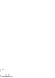
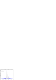
Figure 2: The distribution of eigenvalues $P_{t}(\lambda)$ defined as the ratio between the multiplicity of eigenvalue $\lambda$ and the network order $N_{t}$.

4.2 eigenvectors

Similarly to the eigenvalues, the eigenvectors of $\textbf{A}_{t}$ follow directly from those of $\textbf{A}_{t-1}$. Assume that $\lambda$ is an arbitrary eigenvalue of $U_{t}$, whose corresponding eigenvector is $\textbf{\emph{v}}\in\textbf{R}^{2(m+1)^{t}}$, where $\textbf{R}^{2(m+1)^{t}}$ represents the $2(m+1)^{t}$-dimensional vector space. Then we can solve equation ($\lambda\,\textbf{I}-\textbf{A}_{t})\textbf{\emph{v}}=0$ to find the eigenvector v. We distinguish two cases: $\lambda\in AE^{*}_{t}$ and $\lambda\in AE^{{}^{\prime}}_{t}$, which will be addressed in detail as follows:

For the first case $\lambda\in AE^{*}_{t}$, we can rewrite the equation ($\lambda\,\textbf{I}-\textbf{A}_{t})\textbf{\emph{v}}=0$ as

$$\left(\begin{array}[]{ccccc}\lambda\textbf{I}-\textbf{A}_{t-1}&-\textbf{I}&-\textbf{I}&\cdots&-\textbf{I}\\ -\textbf{I}&\lambda\textbf{I}&{\textbf{0}}&\cdots&{\textbf{0}}\\ -\textbf{I}&{\textbf{0}}&\lambda\textbf{I}&\cdots&{\textbf{0}}\\ \vdots&\vdots&\vdots&&\vdots\\ -\textbf{I}&{\textbf{0}}&{\textbf{0}}&\cdots&\lambda\textbf{I}\end{array}\right)\left(\begin{array}[]{c}\textbf{\emph{v}}_{1}\\ \textbf{\emph{v}}_{2}\\ \textbf{\emph{v}}_{3}\\ \vdots\\ \textbf{\emph{v}}_{m+1}\end{array}\right)=0,$$ (46)

where vector $\textbf{\emph{v}}_{i}$ ($1\leq i\leq m+1$) are components of v. Equation (46) leads to the following equations:

$$\big{(}\lambda\textbf{I}_{t-1}-\textbf{A}_{t-1}\big{)}\textbf{\emph{v}}_{1}-\textbf{\emph{v}}_{2}-\dots-\textbf{\emph{v}}_{m+1}=\textbf{0},$$ (47)

$$-\textbf{\emph{v}}_{1}+\lambda\textbf{\emph{v}}_{i}=\textbf{0}\ \ \ (2\leq i\leq m+1).$$ (48)

Resolve equation (48) to find

$$\textbf{\emph{v}}_{i}=\frac{1}{\lambda}\textbf{\emph{v}}_{1}\ \ (2\leq i\leq m+1).$$ (49)

Substituting equation (49) into equation (47) we have

$$\left[\left(\lambda-\frac{m}{\lambda}\right)\textbf{I}-\textbf{A}_{t-1}\right]\textbf{\emph{v}}_{1}=0,$$ (50)

which indicates that $\textbf{\emph{v}}_{1}$ is the solution of equation (47) while $\textbf{\emph{v}}_{i}$ ($2\leq i\leq m+1$) are uniquely decided by $\textbf{\emph{v}}_{1}$ via equation (49).

From equation (40) in preceding subsection, it is clear that if $\lambda$ is an eigenvalue of adjacency matrix $\textbf{A}_{t}$, then $f(\lambda)=\lambda-\frac{m}{\lambda}$ must be one eigenvalue of $\textbf{A}_{t-1}$. (Recall that if $\lambda=\tilde{\lambda}_{i}^{t}\in AE^{*}_{t}$, then $\varphi(\tilde{\lambda}_{i}^{t})=\lambda_{i}^{t-1}$ for $i\leq 2(m+1)^{t-1}$, or $\varphi(\tilde{\lambda}_{i}^{t})=\lambda_{i-2(m+1)^{t-1}}$ for $i>2(m+1)^{t-1}$). Thus, equation (50) together with equation (40) shows that $\textbf{\emph{v}}_{1}$ is an eigenvector of matrix $\textbf{A}_{t-1}$ corresponding to the eigenvalue $\lambda-\frac{m}{\lambda}$ determined by $\lambda$, while

$$\textbf{\emph{v}}=\left(\begin{array}[]{ccc}\textbf{\emph{v}}_{1}\\ \textbf{\emph{v}}_{2}\\ \textbf{\emph{v}}_{3}\\ \vdots\\ \textbf{\emph{v}}_{m+1}\end{array}\right)=\left(\begin{array}[]{ccc}\textbf{\emph{v}}_{1}\\ \frac{1}{\lambda}\textbf{\emph{v}}_{1}\\ \frac{1}{\lambda}\textbf{\emph{v}}_{1}\\ \vdots\\ \frac{1}{\lambda}\textbf{\emph{v}}_{1}\end{array}\right)$$ (51)

is an eigenvector of $\textbf{A}_{t}$ corresponding to the eigenvalue $\lambda$.

Since for the initial graph $U_{0}$, its adjacency matrix $\textbf{A}_{0}$ has two eigenvalues -1 and 1 with respective eigenvectors $(1,-1)^{\top}$ and $(1,1)^{\top}$. By recursively applying the above process, we can obtain all the eigenvectors corresponding to $\lambda\in AE^{*}_{t}$.

For the second case of $\lambda\in AE^{{}^{\prime}}_{t}$, where all $\lambda=0$, the equation ($\lambda\,\textbf{I}-\textbf{A}_{t})\textbf{\emph{v}}=0$ can be recast as

$$\left(\begin{array}[]{ccccc}-\textbf{A}_{t-1}&-\textbf{I}&-\textbf{I}&\cdots&-\textbf{I}\\ -\textbf{I}&\textbf{0}&{\textbf{0}}&\cdots&{\textbf{0}}\\ -\textbf{I}&{\textbf{0}}&\textbf{0}&\cdots&{\textbf{0}}\\ \vdots&\vdots&\vdots&&\vdots\\ -\textbf{I}&{\textbf{0}}&{\textbf{0}}&\cdots&\textbf{0}\end{array}\right)\left(\begin{array}[]{c}\textbf{\emph{v}}_{1}\\ \textbf{\emph{v}}_{2}\\ \textbf{\emph{v}}_{3}\\ \vdots\\ \textbf{\emph{v}}_{m+1}\end{array}\right)=0,$$ (52)

where vector $\textbf{\emph{v}}_{i}$ ($1\leq i\leq m+1$) are components of v. Equation (52) leads to the following equations:

$$\textbf{\emph{v}}_{1}=\textbf{0},$$ (53)

$$\textbf{\emph{v}}_{2}+\textbf{\emph{v}}_{3}+\dots+\textbf{\emph{v}}_{m+1}=\textbf{0}.$$ (54)

From equation (53), $\textbf{\emph{v}}_{1}$ is a zero vector, and we denote by $\textbf{\emph{v}}_{i,j}$ the $j$-th component of column vector $\textbf{\emph{v}}_{i}$. Equation (54) gives us the following equations:

$$\left\{\begin{array}[]{ccccccccc}\textbf{\emph{v}}_{2,1}&+&\textbf{\emph{v}}_{3,1}&+&\dots&+&\textbf{\emph{v}}_{m+1,1}=\textbf{0}\\ \textbf{\emph{v}}_{2,2}&+&\textbf{\emph{v}}_{3,2}&+&\dots&+&\textbf{\emph{v}}_{m+1,2}=\textbf{0}\\ \vdots&\vdots&\vdots&\vdots&&\vdots&\vdots\\ \textbf{\emph{v}}_{2,2(m+1)^{t-1}}&+&\textbf{\emph{v}}_{3,2(m+1)^{t-1}}&+&\dots&+&\textbf{\emph{v}}_{m+1,2(m+1)^{t-1}}=\textbf{0}\end{array}\right.$$

The set of all solutions to any equation above consists of vectors that can be written as:

$$\left(\begin{array}[]{ccc}\textbf{\emph{v}}_{2,j}\\ \textbf{\emph{v}}_{3,j}\\ \textbf{\emph{v}}_{4,j}\\ \vdots\\ \textbf{\emph{v}}_{m+1,j}\end{array}\right)=k_{1,j}\left(\begin{array}[]{ccc}\textbf{-1}\\ \textbf{1}\\ \textbf{0}\\ \vdots\\ \textbf{0}\end{array}\right)+k_{2,j}\left(\begin{array}[]{ccc}\textbf{-1}\\ \textbf{0}\\ \textbf{1}\\ \vdots\\ \textbf{0}\end{array}\right)+\dots+k_{m-1,j}\left(\begin{array}[]{ccc}\textbf{-1}\\ \textbf{0}\\ \textbf{0}\\ \vdots\\ \textbf{1}\end{array}\right),$$ (55)

where $k_{1,j}$ , $k_{2,j}$ , $\dots$ , $k_{m-1,j}$ are any real numbers. From equation (55), the solutions for all the vectors $\textbf{\emph{v}}_{i}$ ($2\leq i\leq m+1$) can be rewritten as:

$$\left(\begin{array}[]{c}\textbf{\emph{v}}_{2}^{\top}\\ \textbf{\emph{v}}_{3}^{\top}\\ \textbf{\emph{v}}_{4}^{\top}\\ \vdots\\ \textbf{\emph{v}}_{m+1}^{\top}\end{array}\right)=\left(\begin{array}[]{cccc}\textbf{-1}&\textbf{-1}&\cdots&\textbf{-1}\\ \textbf{1}&{\textbf{0}}&\cdots&{\textbf{0}}\\ \textbf{0}&{\textbf{1}}&\cdots&{\textbf{0}}\\ \vdots&\vdots&&\vdots\\ \textbf{0}&{\textbf{0}}&\cdots&\textbf{1}\end{array}\right)\\ \\ \left(\begin{array}[]{cccc}k_{1,1}&k_{1,2}&\cdots&k_{1,2(m+1)^{t-1}}\\ k_{2,1}&k_{2,2}&\cdots&k_{2,2(m+1)^{t-1}}\\ k_{3,1}&k_{3,2}&\cdots&k_{3,2(m+1)^{t-1}}\\ \vdots&\vdots&&\vdots\\ k_{m-1,1}&k_{m-1,2}&\cdots&k_{m-1,2(m+1)^{t-1}}\end{array}\right),$$ (56)

where $k_{i,j}$ ($1\leq i\leq m-1$; $1\leq j\leq 2(m+1)^{t-1}$) are arbitrary real numbers. According to the equation (56), we can obtain the eigenvector v corresponding to the eigenvalue 0. Moreover, it is easy to see that the dimension of the eigenspace of matrix $A_{t}$ associated with eigenvalue 0 is $2(m-1)(m+1)^{t-1}$.

5 Conclusion and discussion

In conclusion, we have studied a family of deterministic models for the uniform recursive tree, which we name the deterministic uniform recursive trees (DURTs) that are constructed in a recursive way. The DURTs are in fact deterministic variants of the intensively studied random uniform recursive tree. We have presented an exhaustive analysis of various structural properties of the DURTs, and obtained the precise solutions for these features that include degree distributions, average path length, betweenness distribution, and degree correlations. Aside from their deterministic structures, the obtained structural characteristics of the DURTs are similar to those of URT. Consequently, the DURTs may provide useful insight to the practices as URT.

Furthermore, by using the methods of linear algebra and graph theory, we have performed a detailed analysis of the complete eigenvalues and their corresponding eigenvectors of the adjacency matrix for DURTs. We have fully characterized the spectral properties and eigenvectors for DURTs. We have shown that all the eigenvalues and eigenvectors of the adjacency matrix for DURTs can be directly determined from those for the initial network. It is expected that the methods applied here can be extended to a larger type of deterministic networks.

References

References

• [1] R. Albert and A.-L. Barabási, Rev. Mod. Phys. 74, 47 (2002).
• [2] S.N. Dorogvtsev and J.F.F. Mendes, Adv. Phys. 51, 1079 (2002).
• [3] M.E.J. Newman, SIAM Rev. 45, 167 (2003).
• [4] L. da. F. Costa, F.A. Rodrigues, G. Travieso, and P.R.V. Boas, Adv. Phys. 56, 167 (2007).
• [5] S. N. Dorogovtsev, A. V. Goltsev and J.F.F. Mendes, Rev. Mod. Phys. 80, 1275 (2008).
• [6] R. Albert, H. Jeong, A.-L. Barabási, Nature (London) 406, 378 (2000).
• [7] D. S. Callaway, M. E. J. Newman, S. H. Strogatz, and D. J. Watts, Phys. Rev. Lett. 85, 5468 (2000).
• [8] R. Cohen, K. Erez, D. ben-Avraham, S. Havlin Phys. Rev. Lett. 86, 3682 (2001).
• [9] Z. Z. Zhang, S. G. Zhou, and T. Zou, Eur. Phys. J. B 56, 259 (2007).
• [10] R. Pastor-Satorras and A. Vespignani, Phys. Rev. Lett. 86, 3200 (2001).
• [11] Z. Z. Zhang, S. G. Zhou, T. Zou, and G. S. Chen, J. Stat. Mech.: Theory Exp. P09008 (2008).
• [12] M. Barahona and L. M. Pecora, Phys. Rev. Lett. 89, 054101 (2002).
• [13] Z. Z. Zhang, L. L. Rong, and S. G. Zhou, Phys. Rev. E, 74, 046105 (2006).
• [14] F. Comellas and S. Gago, J. Phys. A: Math. Theor. 40, 4483 (2007).
• [15] A. Arenas, A. Díaz-Guilera, J. Kurths, Y. Moreno, and C. S. Zhou, Phy. Rep. 469, 93 (2008).
• [16] G. Szabó and G. Fáth, Phy. Rep. 446, 97 (2007).
• [17] A.-L. Barabási, Nat. Phys. 1, 68 (2005).
• [18] I. J. Farkas, I. Derényi, A.-L. Barabási, and T. Vicsek, Phys. Rev. E 64, 026704 (2001).
• [19] K.-I. Goh, B. Kahng, and D. Kim, Phys. Rev. E 64, 051903 (2001).
• [20] S. N. Dorogovtsev, A. V. Goltsev, J. F. F. Mendes, and A. N. Samukhin, Phys. Rev. E 68, 046109 (2003).
• [21] F. Chung, L. Lu, and V. Vu, Proc. Natl. Acad. Sci. U.S.A. 100, 6313 (2003).
• [22] M. Boguñá, R. Pastor-Satorras, and A. Vespignani, Phys. Rev. Lett. 90, 028701 (2003).
• [23] D. Chakrabarti, Y. Wang, C. X. Wang, J. Leskovec, and C. Faloutsos, ACM Trans. Information and System Security, 10, 13 (2008).
• [24] J. G. Restrepo, E Ott and B. R. Hunt, Chaos 16, 015107 (2006).
• [25] G. S. Canright and K. Engø-Mosen, Comlexus, 3, 131 (2006).
• [26] R. T. Smythe, H. Mahmoud, Theor. Probab. Math. Statist. 51, 1 (1995).
• [27] P. Erdös and A. Rényi, Pub. Math. Insti. Hung. Acad. Sci. 5 17 (1960).
• [28] S. N. Dorogovtsev, P. L. Krapivsky, and J. F. F. Mendes, Europhys. Lett. 81, 30004 (2008).
• [29] Z. Z. Zhang, S. G. Zhou, S. H. Zhao, and J. H. Guan, J. Phys. A: Math. Theor. 41, 185101 (2008).
• [30] J. W. Moon, London Math. Soc. Lecture Note 13, 125 (1974).
• [31] D. Najock and C. Heyde, J. Appl. Prob. 19, 675 (1982).
• [32] J. Gastwirth, Amer. Statist. 31, 79 (1977).
• [33] S. Jung, S. Kim, and B. Kahng, Phys. Rev. E 65, 056101 (2002).
• [34] A.-L. Barabási, E. Ravasz, and T. Vicsek, Physica A 299, 559 (2001).
• [35] S.N. Dorogovtsev, A.V. Goltsev, and J.F.F. Mendes, Phys. Rev. E 65, 066122 (2002).
• [36] F. Comellas, G. Fertin and A. Raspaud, Phys. Rev. E 69, 037104 (2004).
• [37] Z. Z. Zhang, L. L. Rong, and S. G. Zhou, Physica A 377, 329 (2007).
• [38] E. Ravasz and A.-L. Barabási, Phys. Rev. E 67, 026112 (2003).
• [39] J. C. Nacher, N. Ueda, M. Kanehisa and T. Akutsu, Phys. Rev. E 71, 036132 (2005).
• [40] J. S. Andrade Jr., H. J. Herrmann, R. F. S. Andrade and L. R. da Silva, Phys. Rev. Lett. 94, 018702 (2005).
• [41] Z. Z. Zhang, L. L. Rong and F. Comellas, J. Phys. A: Math. Gen. 39, 3253 (2006).
• [42] F. Comellas, J. Ozón, and J.G. Peters, Inf. Process. Lett. 76, 83 (2000).
• [43] Z. Z. Zhang, L. L. Rong and C. H. Guo, Physica A 363, 567 (2006).
• [44] M. Hinczewski, Phys. Rev. E 75, 061104 (2007).
• [45] L. Barriére, F. Comellas, and C. Dalfó, J. Phys. A 39, 11739 (2006).
• [46] Z. Z. Zhang, S. G. Zhou, L. J. Fang, J. H. Guan, and Y. C. Zhang, Europhys. Lett. 79, 38007 (2007).
• [47] Z. Z. Zhang, S. G. Zhou, T. Zou, L. C. Chen, and J. H. Guan, Eur. Phys. J. B 60, 259 (2007).
• [48] C. Bedogne, A. P. Masucci, G. J. Rodgers, Physica A 387, 2161 (2008).
• [49] S. Boettcher, B. Gonçalves, and H. Guclu, J. Phys. A: Math. Theor. 41, 252001 (2008).
• [50] L. Barriére, F. Comellas, C. Dalfó, and M. A. Fiol, Linear Algebra Appl. 428, 1499 (2008).
• [51] Z. Z. Zhang, S. G. Zhou, Y. Qi, and J. H. Guan, Eur. Phys. J. B 63, 507 (2008).
• [52] K. I. Goh, E. Oh, H. Jeong, B. Kahng, and D. Kim, Proc. Natl. Acad. Sci. U.S.A. 99, 12583 (2002).
• [53] S.N. Dorogvtsev, J.F.F. Mendes, and J. G. Oliveira, Phys. Rev. E 73, 056122 (2006).
• [54] D. J. Watts and H. Strogatz, Nature (London) 393, 440 (1998).
• [55] M. E. J. Newman, Phys. Rev. E 64, 016132 (2001).
• [56] M. Barthélemy, Eur. Phys. J. B 38, 163 (2004).
• [57] G. Szabó, M. Alava, and J. Kertész, Phys. Rev. E 66, 026101 (2002).
• [58] B. Bollobás and O. Riordan, Phys. Rev. E 69, 036114 (2004).
• [59] C.-M. Ghima, E. Oh, K.-I. Goh, B. Kahng, and D. Kim, Eur. Phys. J. B 38, 193 (2004)
• [60] Z. Z. Zhang, S. G. Zhou, L. C. Chen, J. H. Guan, L. J. Fang, and Y. C. Zhang, Eur. Phys. J. B 59, 99 (2007).
• [61] Z. Z. Zhang, S. G. Zhou, L. C. Chen, and J. H. Guan, Eur. Phys. J. B 64, 277 (2008).
• [62] A.-L. Barabási and R. Albert, Science 286, 509 (1999).
• [63] S. Maslov and K. Sneppen, Science 296, 910 (2002).
• [64] R. Pastor-Satorras, A. Vázquez and A. Vespignani, Phys. Rev. Lett. 87, 258701 (2001).
• [65] A. Vázquez, R. Pastor-Satorras and A. Vespignani, Phys. Rev. E 65, 066130 (2002).
• [66] Z. Z. Zhang and S. G. Zhou, Physica A, 380, 621 (2007).
• [67] M. E. J. Newman, Phys. Rev. Lett. 89, 208701 (2002).
• [68] J. R. Silvester, Math. Gaz. 84, 460 (2000).