Worldsheet Analysis of Gauge/Gravity Dualities

abstract

Gauge/gravity dualities are investigated from the worldsheet point of view. In [3], a duality between 4d SYM and supergravity on $AdS_{5}\times S^{5}$ has been partly explained by using an anisotropic scale invariance of worldsheet theory. In this paper, we refine the argument and generalize it to lower dimensional cases. We show the correspondence between the Wilson loops in $(p+1)$-d SYM and the minimal surface in the black $p$-brane background. Although the scale invariance does not exist in these cases, the generalized scale transformation can be utilized. We also find that the energy density of open strings can be related to the ADM mass of the $p$-brane without relying on this symmetry.

1 Introduction

Since the AdS/CFT correspondence has been conjectured [2], many evidences have been found and various applications have been proposed by assuming its correctness. However, it is still not clear to what extent this correspondence holds.

As a concrete example, let us consider the original $AdS_{5}\times S^{5}$ setup. In the narrowest sense, it is conjectured that 4d ${\cal N}=4$ super Yang-Mills theory (SYM) is equivalent to type IIB supergravity on the $AdS_{5}\times S^{5}$ background, in the large-$N$ and strong ’t Hooft coupling limit. From various nontrivial checks, the conjecture seems to be correct at least in this limit. This correspondence is often extended to finite ’t Hooft coupling, for which the SYM corresponds to type IIB string theory in the classical limit. In some cases, correspondence between finite-$N$ SYM and fully quantized type IIB string is considered. However, it is not apparent whether it really holds in such a wider sense. It is also not clear whether the duality between theories with lower symmetries can hold. Clarification of such issues is crucial for correct application of the duality. String worldsheet viewpoint is expected to shed light on these questions and may provide a proof of the duality.

In [3], a part of the narrowest correspondence is explained by considering worldsheets of strings propagating in the background of $N$ coincident D3-branes . The essential point is that an anisotropic scale invariance holds as long as worldsheets are located in the near horizon region. This symmetry can be used to directly relate SYM to supergravity. If we introduce a source D-brane close to the D3-branes, the string worldsheets stretched between them can be regarded as a Wilson loop in $\mathcal{N}=4$ $SU(N)$ SYM. By applying the scale transformation so that the source D-brane is distant from the D3-branes but still in the near horizon region, this system is described by supergravity on the $AdS_{5}\times S^{5}$ background. In this way, SYM and supergravity are related to each other by the scale transformation.

In [5], it is proposed that there are dualities between $(p+1)$-d SYM and type II string theory on black $p$-brane background for $p\neq 3$. At large-$N$ and strong ’t Hooft coupling, the energy density and Wilson loop in SYM are conjectured to correspond to the ADM mass and a minimal surface of string worldsheet in the gravity side [6]. In this case, SYM is not conformal and the background in the gravity side is not AdS. However, recent numerical simulations for $p=0$ SYM [7, 8, 9, 10] support the validity of the correspondence.

In this paper, we refine the proposal of [3] and generalize it to lower dimensional D$p$-branes and of finite temperature. We notice that the near horizon geometries of these branes do not have the scale transformation as an isometry. To see the correspondence of the energy density, it turns out that no symmetries are needed. By examining the origin of the ADM mass, we can show that it is exactly equal to the energy of the D-brane system. In the near extremal limit, the system is described by SYM. Then, by subtracting the D-brane tension from the ADM mass, we obtain the energy density of SYM.

For the Wilson loops, a certain symmetry is needed to relate the gravity side to SYM side. For this purpose we use the generalized scale transformation proposed in [11]. The near horizon geometry of the black $p$-brane [12] in the unit $\alpha^{\prime}=1$ is given by

$$ds^{2}=\Bigl{(}\frac{U^{7-p}}{d_{p}\lambda}\Bigr{)}^{\frac{1}{2}}\Bigl{[}\Bigl{(}1-\Bigl{(}\frac{U_{0}}{U}\Bigr{)}^{7-p}\Bigr{)}dx_{p+1}^{2}+\displaystyle{\sum_{a=1}^{p}}dx_{a}^{2}\Bigr{]}+\Bigl{(}\frac{d_{p}\lambda}{U^{7-p}}\Bigr{)}^{\frac{1}{2}}\Bigl{[}\frac{dU^{2}}{1-\Bigl{(}\frac{U_{0}}{U}\Bigr{)}^{7-p}}+U^{2}d\Omega_{8-p}^{2}\Bigr{]}.$$ (1.1)

This geometry is invariant under the following transformation;

$$x_{A}\ \to c^{-1}x_{A}\quad(A=1,2,\cdots,p,p+1),$$ (1.2)

$$U\ \to cU,$$ (1.3)

$$\lambda\ \to c^{3-p}\lambda,$$ (1.4)

where $c$ is a real and positive parameter. As we will see, in the near horizon region, the generalized scale transformation turns out to be a stringy symmetry. We then consider a configuration in which the source D-brane is widely extended and located close to the D$p$-branes, as shown in the left picture in figure 1. In this case the Wilson loop is described by the low energy effective theory of the open strings, that is, SYM. Then we apply the generalized scale transformation so that the worldsheet is stretched in the vertical direction and shrunk in the horizontal direction, as in the middle picture in figure 1. Then, as in the right picture, the amplitude can be evaluated as the area of the minimal surface in the black $p$-brane background. If we locate the source D-brane sufficiently close to the D$p$-branes in the original configuration, we can keep it in the near horizon region during the deformation. In this way, the gauge/gravity correspondence follows simply, once we can show the invariance.

Figure 1: The Wilson loop in SYM is represented by the string worldsheets stretching between a source D-brane and the $N$ coincident D-branes (left). By the generalized scale transformation, the source D-brane is lifted away from the $N$ D-branes but still in the near horizon region (middle). This diagram can be evaluated as a minimal surface in a curved background (right).

This paper is organized as follows. In section 2, we examine the correspondence between the energy density of SYM and the ADM mass of the black $p$-brane without using any symmetries. In section 3, we discuss the generalized scale transformation and show the correspondence between the Wilson loop in SYM and the minimal surface in supergravity by applying the transformation. Section 4 is devoted to conclusions and discussions.

2 Energy Density and ADM Mass

In this section we discuss the correspondence of the entropy. We show it by directly comparing the energy density of the D$p$-branes and the ADM mass in the asymptotically flat region. We do not rely on any symmetry here. It is in contrast to the case of the Wilson loops which we will discuss in the next section.

We start with considering the system of open strings on the D$p$-branes at finite temperature. We do not impose a constraint that it is reduced to SYM. If we observe the system at a point distant from the D$p$-branes, the space-time is almost flat and described by supergravity. However, if we come closer to the D$p$-branes, in principle two types of corrections will come in. One is the quantum gravity effect and the other is the $\alpha^{\prime}$ correction or stringy effect. We suppress them by imposing the condition

$$\beta\gg 1,\quad\lambda\gg 1,\quad\text{and}\quad N\to\infty,$$ (2.5)

where $\beta$ is the inverse temperature. The large-$N$ limit, $N\to\infty$ with $\lambda=(2\pi)^{p-2}g_{s}N$ kept fixed, suppresses closed string loops, and the conditions $\lambda\gg 1$ and $\beta\gg 1$ guarantee that the curvature is small everywhere outside the event horizon.

In general, the ADM mass is obtained by observing the gravitational field in the asymptotically flat region. We regard the deviation of the metric from the flat one as a graviton in the weak field expansion, and the ADM mass is calculated from the linearized Einstein equation assuming that the source of the graviton is the energy-momentum tensor. In order to apply this procedure, we first attach a tube of a closed string to the open string worldsheet so that we can observe the system from the asymptotically flat region (see, for example, the left diagram of figures 2 and 3). When the observer is distant from the D$p$-branes, this tube becomes propagation of massless bosons, and represents the deviation of the metric from the flat space.

Let us consider a few examples. First we consider the contribution from the disk diagram (left diagram of Figure 2). If we observe it in the asymptotically flat region, the amplitude is replaced by the right diagram in figure 2, that is, a disk amplitude with a vertex insertion. This amplitude is independent of the temperature because it does not wrap on the temporal circle, and is proportional to $\frac{1}{U^{7-p}}$, where $U$ stands for the location of the observer. ($U^{-8}$ from a propagator and $U^{p+1}$ from an integral over the location of the disk.)

The second simplest diagram is the cylinder, which is regarded as a sum of two amplitudes as shown in figure 3. The middle diagram is similar to that appeared in the previous example, while the right is the one-loop vacuum diagram of open strings with an emission vertex attached. The middle diagram is independent of the temperature and behaves as $\frac{1}{U^{2(7-p)}}$ ($U^{-8\times 3}$ from three propagators, $U^{-2}$ from a three point vertex in the bulk, $U^{10}$ from the location of the three point vertex and $U^{(p+1)\times 2}$ from two integrals over the location of the disks). The right one behaves as $\frac{1}{U^{7-p}}$ and depends on temperature. Especially it vanishes at zero temperature as a result of supersymmetry. We can discuss worldsheets with more boundaries in a similar manner.

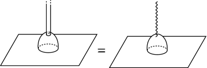
Figure 2: A disk amplitude (left). We attached a long thin tube to the worldsheet.

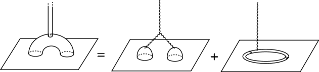
Figure 3: A cylinder amplitude (left) are regarded as two diagrams: a diagram corresponding to the mass of the D$p$-branes (middle); a one-loop diagram corresponding to the energy density of the open strings (right).

Because the solution of the supergravity is uniquely determined by the mass, RR charge and isometry, the sum of these contributions should reproduce the black $p$-brane solution

$$ds^{2} = f_{p}^{-\frac{1}{2}}\Bigl{[}\Bigl{(}1-\Bigl{(}\frac{U_{0}}{U}\Bigr{)}^{7-p}\Bigr{)}dx_{p+1}^{2}+\displaystyle{\sum_{a=1}^{p}}dx_{a}^{2}\Bigr{]}+f_{p}^{\frac{1}{2}}\Bigl{[}\frac{dU^{2}}{1-(\frac{U_{0}}{U})^{7-p}}+U^{2}d\Omega_{8-p}^{2}\Bigr{]},$$

$$e^{\phi} = g_{s}f_{p}^{\frac{3-p}{4}},$$ (2.7)

$$A_{1,\cdots,p,p+1} = \frac{1}{2g_{s}}(f_{p}^{-1}-1),$$ (2.8)

where

$$f_{p}=1+\frac{\alpha_{p}d_{p}\lambda}{U^{7-p}},$$ (2.9)

$$\alpha_{p}=\sqrt{1+\Bigl{(}\frac{U_{0}^{7-p}}{2d_{p}\lambda}\Bigr{)}^{2}}-\Bigl{(}\frac{U_{0}^{7-p}}{2d_{p}\lambda}\Bigr{)}, d_{p}=2^{7-p}\pi^{\frac{9-3p}{2}}\Gamma\Bigl{(}\frac{7-p}{2}\Bigr{)}.$$ (2.10)

Here $x_{p+1}$ is the Euclidean time, and compactified as $x_{p+1}\sim x_{p+1}+\beta$.

For example, the $(p+1,p+1)$-component of (LABEL:metric_finite) is expanded as

$$g_{p+1{\ }p+1}=1-\left(\frac{1}{2}\alpha_{p}d_{p}\lambda-U_{0}^{7-p}\right)\frac{1}{U^{7-p}}+\mathcal{O}\Bigl{(}\frac{1}{U^{2(7-p)}}\Bigr{)}.$$ (2.11)

The right diagrams in figure 2 and in figure 3 represent parts of the second term, while the middle diagram in figure 3 corresponds to the higher order terms.

In other words, the sum of the worldsheet amplitudes converges for large enough $U$, and can be analytically continued to smaller $U$ as (LABEL:metric_finite). However, there are two possibilities about the event horizon.

1. The D$p$-branes form a black $p$-brane. In this case, the horizon radius $U_{0}$ is determined by $\beta$ from the absence of conical singularity as usual:

   $$\beta=\frac{4\pi U_{0}}{(7-p)}\Bigl{(}1+\frac{\alpha_{p}d_{p}\lambda}{U_{0}^{7-p}}\Bigr{)}^{\frac{1}{2}}.$$ (2.12)

2. The D$p$-branes form an extended object, and we have no event horizon. In this case we can trust the solution (LABEL:metric_finite) only outside the object, and a dynamical analysis of the D$p$-branes is needed to determine $U_{0}$.

In any case, the ADM mass is determined by the asymptotic $1/U^{7-p}$ behavior of the fields. We formally integrate the $(p+1,p+1)$-component of the energy momentum tensor $T_{\mu\nu}$ and extract the surface term at infinity. Here $T_{\mu\nu}$ is defined by the weak field expansion of the Einstein equation:

$$T_{\mu\nu}=\frac{1}{2\kappa^{2}}\Bigl{(}\partial_{\mu}\partial_{\alpha}h^{\alpha}_{{\ }\nu} + \partial_{\nu}\partial_{\alpha}h^{\alpha}_{{\ }\mu}-\partial_{\alpha}\partial^{\alpha}h_{\mu\nu}-\partial_{\mu}\partial_{\nu}h^{\alpha}_{{\ }\beta}$$ (2.13)

$$- \eta_{\mu\nu}(\partial_{\alpha}\partial_{\beta}h^{\alpha\beta}-\partial_{\alpha}\partial^{\alpha}h^{\beta}_{{\ }\beta})+4(\partial_{\mu}\partial_{\nu}\phi-\eta_{\mu\nu}\partial_{\alpha}\partial^{\alpha}\phi)\Bigr{)}.$$

In the Einstein frame $h_{\mu\nu}^{E}=h_{\mu\nu}-\frac{1}{2}\eta_{\mu\nu}\phi$, this becomes

$$T_{\mu\nu}=\frac{1}{2\kappa^{2}}\Bigl{(}\partial_{\mu}\partial_{\alpha}{h^{E}}^{\alpha}_{{\ }\nu}+\partial_{\nu}\partial_{\alpha}{h^{E}}^{\alpha}_{{\ }\mu}-\partial_{\alpha}\partial^{\alpha}{h^{E}}_{\mu\nu}-\partial_{\mu}\partial_{\nu}{h^{E}}^{\alpha}_{{\ }\beta}-\eta_{\mu\nu}(\partial_{\alpha}\partial_{\beta}{h^{E}}^{\alpha\beta}-\partial_{\alpha}\partial^{\alpha}{h^{E}}^{\beta}_{{\ }\beta})\Bigr{)}.$$ (2.14)

The ADM mass (per unit volume of the D$p$-branes) thus obtained is

$$M=\frac{N^{2}}{4\pi^{2}(7-p)d_{p}\lambda^{2}}\Bigl{(}(8-p)U_{0}^{7-p}+(7-p)\alpha_{p}d_{p}\lambda\Bigr{)}.$$ (2.15)

If we set $U_{0}=0$, we have the zero temperature limit $M_{0}=\frac{N^{2}}{4\pi^{2}\lambda}$, which is nothing but the tension of the $N$ D$p$-branes and corresponds to the disk diagram depicted in figure 2. The rest $M-M_{0}$ comes from the vacuum amplitudes of open strings. The “mixed” diagrams do not contribute to the ADM mass, because they are of order $\mathcal{O}(\frac{1}{U^{2(7-p)}})$ as in the middle diagram in figure 3.

We can directly show the equivalence of the ADM mass and the energy of the open string system. In general, the ADM mass is defined as the source of the graviton in the weak field expansion. As we have seen in figure 2 and 3, in our case, it is nothing but the expectation value of the graviton emission vertex. There might be a doubt about the use of the weak field expansion near the D$p$-branes, since the space-time is curved there. However, this treatment is correct for the calculation of the ADM mass, because what we need are processes of single graviton emission as the right diagram of figure 3. Then the coupling of the graviton to the open strings in the leading order of the weak field expansion is obtained by setting the target space metric to

$$G_{\mu\nu}=\delta_{\mu\nu}+h_{\mu\nu},$$ (2.16)

in the worldsheet action of the string. Therefore the source $T_{\mu\nu}$ of the graviton in (2.13) is equal to the energy momentum tensor of the open strings on the flat D$p$-branes.

2.1 Low Temperature Limit - Gauge/Gravity Correspondence

As we have discussed, it is not clear whether the event horizon is really formed or not. However, if $p\leq 3$ and the temperature is low enough, we have a rather strong evidence for its formation. In the low temperature limit, the open strings on the D$p$-branes can be described by SYM. Since SYM is finite for $p\leq 3$, the energy density is given by dimensional analysis as

$$M=M_{0}+\beta^{-p-1}f(\lambda\beta^{3-p}).$$ (2.17)

On the gravity side, if we assume the existence of the event horizon, we can determine $U_{0}$ as a function of $\beta$ by using (2.12) and then the energy density using (2.15). First, we consider the near extremal region

$$U_{0}^{7-p}\ll d_{p}\lambda,$$ (2.18)

which is equivalent to

$$\beta\gg\lambda^{\frac{1}{7-p}},$$ (2.19)

as long as (2.12) is satisfied. Then (2.12) is solved as $U_{0}=const.\times\left(\frac{\lambda}{\beta^{2}}\right)^{\frac{1}{5-p}}$ and (2.15) gives

$$M=M_{0}+const.\times\beta^{-p-1}\left(\lambda\beta^{3-p}\right)^{-\frac{3-p}{5-p}},$$ (2.20)

which has the form of (2.17). Thus we have seen that the consequences of two assumptions agree in a non-trivial manner. One is that the open strings form the event horizon, and the other is that they are described by SYM in the low temperature region. Therefore it is natural to conclude that both assumptions are correct.

On the other hand, if the condition (2.19) is not satisfied, the energy density obtained from (2.12) and (2.15) no longer satisfies (2.17). Therefore either of the two assumptions breaks down.

2.2 Open String/Gravity Correspondence

In this section, we assume that the event horizon is always there for any temperature. Then we can trust (2.12) for any $\beta$ and regard it as expressing the duality between the open string system that is not necessarily reduced to SYM and the classical gravity.

To make the situation clearer, we rewrite (2.12) in terms of scaling variables

$$b=\frac{4\pi u_{0}}{7-p}\left(\frac{1}{2}+\frac{1}{2}\sqrt{1+\left(\frac{1}{u_{0}^{7-p}}\right)^{2}}\right)^{\frac{1}{2}},$$ (2.21)

where

$$b = \frac{\beta}{(2d_{p}\lambda)^{\frac{1}{7-p}}},$$ (2.22)

$$u_{0} = \frac{U_{0}}{(2d_{p}\lambda)^{\frac{1}{7-p}}}.$$ (2.23)

As is shown in figure 4, two values of $u_{0}$ correspond to the same temperature, if $p<5$. If $u_{0}\ll 1$, the system is described by SYM and the temperature behaves as $b^{-1}\sim u_{0}^{\frac{5-p}{2}}$. If we keep increasing the energy, the horizon radius $u_{0}$ becomes larger, while the temperature $b^{-1}$ becomes maximum $b_{c}^{-1}$ at $u_{0}=u_{c}$, and then decreases to zero.

Figure 4: Black $p$-brane temperature as a function of the horizon radius in the case $p<5$

Let us see what happens to the system of open strings when the energy is increased from zero to infinity. At the beginning when $u_{0}\ll 1$, the open strings are in a low energy state and described by SYM. When we increase the energy, stringy excitations become important and the system is no longer described by SYM, but still we can imagine it as a gas of open strings. However, this picture breaks down when the temperature reaches the maximum value $b_{c}^{-1}$, beyond which the heat capacity becomes negative. Although this transition is reminiscent of the Hagedorn transition, some differences are there. Firstly, this transition is caused by the interaction between the open strings. In fact, the maximum temperature $T_{max}$ becomes lower as $\lambda$ is increased as is seen from (2.23):

$$T_{max}=\frac{1}{b_{c}(2d_{p}\lambda)^{\frac{1}{7-p}}}.$$ (2.24)

Secondly the negative heat capacity indicates that the density of states becomes even larger if we further increase the energy, which is contrary to what is expected from the Hagedorn transition [13]. We finally comment that the metric (LABEL:metric_finite) becomes the Schwarzschild metric for large values of $u_{0}$, so that Schwarzschild black hole is realized as a system of dense and strongly coupled open strings.

3 Wilson Loop and Minimal Surface

In this section, we discuss the correspondence of Wilson loops. The procedure is analogous to that in [3] and we use a worldsheet symmetry to relate SYM side and the gravity side directly. For a while, we discuss the zero temperature case.

To find the symmetry, we examine the black $p$-brane solution at zero temperature, which is written as (LABEL:metric_finite) with $U_{0}$ set to zero. In the near horizon region

$$U^{7-p}\ll d_{p}\lambda,$$ (3.25)

it becomes

$$ds^{2}=\Bigl{(}\frac{U^{7-p}}{d_{p}\lambda}\Bigr{)}^{\frac{1}{2}}\Bigl{[}dx_{p+1}^{2}+\displaystyle{\sum_{a=1}^{p}}dx_{a}^{2}\Bigr{]}+\Bigl{(}\frac{d_{p}\lambda}{U^{7-p}}\Bigr{)}^{\frac{1}{2}}\Bigl{[}dU^{2}+U^{2}d\Omega_{8-p}^{2}\Bigr{]}.$$ (3.26)

This metric is invariant under the generalized scale transformation

$$x_{A}\ \to c^{-1}x_{A}\quad(A=1,2,\cdots,p+1),$$ (3.27)

$$U,\ \to cU,$$ (3.28)

$$\lambda\ \to c^{3-p}\lambda.,$$ (3.29)

where $c$ is an arbitrary real positive number. Here we have checked the symmetry in the supergravity limit. However, as we will see below, it holds in the stringy level provided that the worldsheet is planar and located within the near horizon region and that $\lambda\gg 1$.

The Wilson loop is given by a power series of $\lambda$ as

$$W(\lambda)=\displaystyle{\sum_{n=0}^{\infty}}\frac{\lambda^{n-1}}{n!}W_{n}.$$ (3.30)

Here $W_{n}$ is the contribution of the worldsheet that has $n$ boundaries corresponding to the coincident $N$ D$p$-branes and one boundary corresponding to the source D-brane as depicted in figure 5. At each solid circle we impose the boundary condition that corresponds to the D$p$-brane, and give factor $N$. At the dashed circle we take the boundary condition for the source D-brane which creates the Wilson loop.

Before showing the invariance of the Wilson loop, we mention how the gauge/gravity correspondence is shown by this symmetry. We start with a configuration in which the source D-brane is widely extended and located close to the D$p$-branes, as shown in the left picture in figure 1. In this case the Wilson loop is described by the low energy effective theory of the open strings, that is, SYM. Then we apply the generalized scale transformation so that the worldsheet is stretched in the vertical direction and shrunk in the horizontal direction, as in the middle picture in figure 1. Then, as in the right picture, the amplitude can be evaluated as the area of the minimal surface in the black $p$-brane background. If we locate the source D-brane sufficiently close to the D$p$-branes in the original configuration, we can keep it in the near horizon region during the deformation. In this way, the gauge/gravity correspondence follows simply, once we can show the invariance.

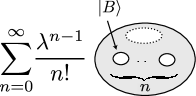
Figure 5: A Wilson loop in terms of the worldsheets.

3.1 Scale Transformation of Boundaries

Let us examine how the boundaries transform under the scale transformation . In the Green-Schwarz formalism, the boundary state of the D$p$-branes is given by

$$|B(p,X_{i})\rangle = \exp\Biggl{[}\displaystyle{\sum_{n=1}^{\infty}}\Bigl{(}\frac{1}{n}M^{ij}\alpha^{i}_{-n}\tilde{\alpha}^{j}_{-n}-iM^{ab}S^{a}_{-n}\tilde{S}^{b}_{-n}\Bigr{)}\Biggr{]}|B_{0}\rangle,$$ (3.31)

$$|B_{0}\rangle = C|p_{A}=0\rangle|x_{i}=X_{i}\rangle\Bigl{(}M^{ij}|i\rangle|\tilde{j}\rangle-M^{\dot{a}\dot{b}}|\dot{a}\rangle|\dot{b}\rangle\Bigr{)}\displaystyle{\bigotimes_{n=1}^{\infty}}|0_{n}\rangle,$$ (3.32)

where $C$ is a constant and $X_{i}$ is the location of the D$p$-branes [14]. $M^{ij}$, $M^{ab}$ and $M^{\dot{a}\dot{b}}$ are defined by

$$M^{ij} = \left(\begin{array}[]{cc}-\mathbf{1}_{p+1}&0\\ 0&\mathbf{1}_{7-p}\\ \end{array}\right),$$ (3.35)

$$M^{ab} = (\gamma_{1}\cdots\gamma_{p+1})^{ab},\quad M^{\dot{a}\dot{b}}=(\gamma_{1}\cdots\gamma_{p+1})^{\dot{a}\dot{b}}.$$ (3.36)

Under the infinitesimal scale transformation $c=1+\epsilon$, worldsheet coordinates, their conjugate momenta and their super partners transform as

$$\delta X^{i}(\sigma)=\epsilon M^{ij}X^{j},\quad\delta P^{i}(\sigma)=-\epsilon M^{ij}P^{j},$$ (3.37)

$$\delta S^{a}(\sigma)=i\epsilon M^{ab}\tilde{S}^{b},\quad\delta\tilde{S}^{a}(\sigma)=-i\epsilon M^{ab}S^{b},$$ (3.38)

or, in terms of the modes we have

$$\delta\alpha_{n}^{i}=-\epsilon M^{ij}\tilde{\alpha}_{-n}^{j},\quad\delta\tilde{\alpha}_{n}^{i}=-\epsilon M^{ij}\alpha_{-n}^{j},$$ (3.39)

$$\delta S_{n}^{a}=i\epsilon M^{ab}\tilde{S}_{-n}^{b},\quad\delta\tilde{S}_{n}^{a}=-i\epsilon M^{ab}S_{-n}^{b}.$$ (3.40)

The exponential factor of the RHS of (3.31) is invariant under this transformation due to the supersymmetry, and only the zero mode part (3.32) gives a nontrivial factor. In order to determine this factor, we consider the low energy limit, that is, SYM. By a simple power counting we can show that the Feynman diagrams of SYM corresponding to $W_{n}$ are proportional to $L^{(3-p)(n-1)}$, where $L$ is the size of the Wilson loop (see figure 6). For example, in the SYM limit, $W_{1}$ becomes $1$, and $W_{2}$ represents one-boson exchange and is of order $L^{(3-p)}$. Because $L$ transforms as $x_{A}$ (3.27), we find that the contribution to the scale transformation coming from the boundaries is given by $c^{-(3-p)(n-1)}$.

Therefore if we apply the scale transformation (3.39) and (3.40) to the Wilson loop (3.30), the factor coming from the boundaries is exactly cancelled by that from $\lambda^{n-1}$, provided that $\lambda$ is transformed as (3.29). Then the variation of the Wilson loop simply comes from that of the worldsheet action.

Figure 6: Feynman diagrams of SYM corresponding to $W_{n}$. The dotted and wavy lines represent the contour of the Wilson loop and a boson propagator respectively.

3.2 Scale Transformation of Wilson Loops

The variation of the worldsheet action is expressed as an insertion of the vertex operator that corresponds to the level zero part $|B_{0}\rangle$ of the boundary state of the D$p$-branes [3]. In order to evaluate such insertion, we introduce an extra D$p$-brane that is placed at $X_{i}=z_{i}$ $(i=p+2,\cdots,10)$. By $W_{n+1}(z)$ we denote the worldsheet of $W_{n}$ with one extra boundary added that correspond to the D$p$-brane placed at $X_{i}=z_{i}$ (see the right picture of figure 7). Then the operator insertion is expressed by an LSZ-like formula [3]

$$\delta_{S}W_{n}=\epsilon\int d^{9-p}z\Delta_{z}W_{n+1}(z).$$ (3.41)

Here $\delta_{S}$ stands for the variation coming from that of the worldsheet action. By summing up for $n$, we have

$$\delta_{S}W(\lambda) = \epsilon\int d^{9-p}z\Delta_{z}W(\lambda,z),$$ (3.42)

$$W(\lambda,z) = \displaystyle{\sum_{n=0}^{\infty}}\frac{\lambda^{n-1}}{n!}W_{n+1}(z).$$ (3.43)

Suppose that the source D-brane is located at a distance $h$ from the $N$ D$p$-branes. Then the worldsheet is stretched approximately in a region $0\leq|X_{i}|\leq U$, where $U=\text{max}(l_{s},h)$. For $0\leq|z_{i}|\leq U$, we assume that $W(\lambda,z)$ varies slowly with $|z_{i}|$, that is,

$$W(\lambda,z)\sim W(\lambda,0).$$ (3.44)

When $z_{i}$ is larger than $U$ but inside the near horizon region, the tube stretching to the boundary at $X_{i}=z_{i}$ becomes thin and it is described by a propagation of massless states of closed string. Therefore

$$W(\lambda,z)\sim\frac{U^{7-p}}{z^{7-p}}W(\lambda,z=U)\sim\frac{U^{7-p}}{z^{7-p}}W(\lambda,z=0),$$ (3.45)

for $|z_{i}|\geq U$.

From the last estimate, (3.42) is evaluated as

$$\delta_{S}W(\lambda)\sim\epsilon U^{7-p}W(\lambda,z=0)=\frac{\epsilon U^{7-p}}{\lambda}\partial_{\lambda}(\lambda W(\lambda)).$$ (3.46)

Here we have used the identity

$$W(\lambda,z=0)=\frac{\partial_{\lambda}(\lambda W(\lambda))}{\lambda},$$ (3.47)

which follows from $W_{n+1}(z=0)=W_{n+1}$. Therefore we obtain

$$\delta_{S}\log(\lambda W(\lambda))\sim\epsilon U^{7-p}\partial_{\lambda}\log(\lambda W(\lambda))<\frac{\epsilon U^{7-p}}{\lambda}\log(\lambda W(\lambda)),$$ (3.48)

which indicates $\delta_{S}W(\lambda)$ is negligible compared to the Wilson loop $W(\lambda)$ itself, if the source D-brane is located in the near horizon region $U^{7-p}\ll\lambda$. Here we have assumed that $\log(\lambda W(\lambda))$ is bounded by a polynomial for large $\lambda$ so that $\partial_{\lambda}\log(\lambda W(\lambda))$ is bounded by $\log(\lambda W(\lambda))/\lambda$.

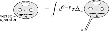
Figure 7: A pictorial description of LSZ-like method.

3.3 Generalization to Finite Temperature

Generalization to the case of finite temperature is straightforward. In the supergravity limit, the black $p$-brane solution at finite temperature is written as (LABEL:metric_finite) and in the near horizon region (3.25) it becomes

$$ds^{2}=\Bigl{(}\frac{U^{7-p}}{d_{p}\lambda}\Bigr{)}^{\frac{1}{2}}\Bigl{[}\Bigl{(}1-\Bigl{(}\frac{U_{0}}{U}\Bigr{)}^{7-p}\Bigr{)}dx_{p+1}^{2}+\displaystyle{\sum_{a=1}^{p}}dx_{a}^{2}\Bigr{]}+\Bigl{(}\frac{d_{p}\lambda}{U^{7-p}}\Bigr{)}^{\frac{1}{2}}\Bigl{[}\frac{dU^{2}}{1-(\frac{U_{0}}{U})^{7-p}}+U^{2}d\Omega_{8-p}^{2}\Bigr{]}.$$

(3.49)

Here we have also assumed the near extremal limit (2.18) in order that the event horizon is inside the near horizon region. This metric is invariant under the generalized scale transformation

$$x_{A}\ \to c^{-1}x_{A}\quad(A=1,2,\cdots,p,p+1),$$ (3.50)

$$U,\quad U_{0} \to cU,\quad cU_{0}$$ (3.51)

$$\lambda\ \to c^{3-p}\lambda,$$ (3.52)

where $c$ is an arbitrary real positive number.

We can show that this symmetry is extended to the stringy level as in the zero-temperature case. The boundary state of the D$p$-branes at finite temperature is given by [15],

$$|B(p,X^{i})\rangle = \exp\Biggl{[}\displaystyle{\sum_{n=1}^{\infty}}\Bigl{(}\frac{1}{n}M^{ij}\alpha^{i}_{-n}\tilde{\alpha}^{j}_{-n}-iM^{ab}S^{a}_{-n}\tilde{S}^{b}_{-n}\Bigr{)}\Biggr{]}|B_{0}\rangle,$$ (3.53)

$$|B_{0}\rangle = C\beta\displaystyle{\sum_{w\in\mathbf{Z}}}e^{i\theta w}|w\rangle|p_{a}=0,n_{KK}=0\rangle|x^{i}=X^{i}\rangle\Bigl{(}M^{ij}|i\rangle|\tilde{j}\rangle-M^{\dot{a}\dot{b}}|\dot{a}\rangle|\dot{b}\rangle\Bigr{)}\displaystyle{\bigotimes_{n=1}^{\infty}}|0_{n}\rangle,$$

where $w$ is the winding number, $n_{KK}$ is the Kaluza-Klein momentum and $\theta$ is an expectation value of the Wilson line along the Euclidean time direction. Under the scale transformation, this state transforms in the same manner as that of zero temperature, and we can apply the same analysis to show the invariance of the Wilson loop as before.

Then by using the transformation, we can relate the SYM side to the supergravity side. The only thing we need to check is the validity of the classical supergravity, which we discuss below.

3.4 Validity of the Classical Gravity

Using the generalized scale transformation, we can show that the Wilson loop in SYM (the left in figure 1) is equivalent to the long-stretched worldsheet (the middle in figure 1). In this subsection we examine when the latter can be evaluated by classical gravity.

For simplicity, we consider the Polyakov line here. We assume that the source D-brane is placed sufficiently distant from the event horizon $h\gg U_{0}$, where $h$ is the distance between the source D-brane and the D$p$-branes. First, the conditions (2.5) must be satisfied after the transformation in order for classical gravity to be applicable. Hence the scaling factor $c$ should satisfy

$$c^{-1}\beta\gg 1,\qquad c^{3-p}\lambda\gg 1,$$ (3.55)

or equivalently,

$$\lambda^{-1/(3-p)}\ll c\ll\beta.$$ (3.56)

In order for $c$ to exist we need

$$\beta^{3-p}\lambda\gg 1.$$ (3.57)

Note that $\beta^{3-p}\lambda$ is invariant under the generalized scale transformation, and can be regarded as the effective coupling constant of SYM as in (2.17).

Next, we require that after the transformation the source D-brane is located sufficiently far from the D$p$-branes so that the stringy excitations are suppressed around the minimal surface. At the same time it must be in the near horizon region in order for the generalized scale transformation to be applicable. Therefore, we need

$$1\ll ch,\qquad ch\ll(c^{3-p}\lambda)^{1/(7-p)},$$ (3.58)

or equivalently,

$$h^{-1}\ll c\ll\lambda^{1/4}h^{-(7-p)/4}.$$ (3.59)

In summary, the classical gravity is valid when (3.56) and (3.59) are satisfied. It is easy to check that such $h$ and $c$ exist if (3.57) is satisfied, assuming $p\leq 3$. Then the right picture in figure 1 can be evaluated as the area of the minimal surface in the black $p$-brane background.

4 Conclusions and Discussions

In this paper, we investigated gauge/gravity dualities from the worldsheet viewpoint. We directly related SYM to supergravity by analyzing worldsheets.

For the energy density or entropy, we have considered open strings on the D-branes and a single graviton emission from them. We identified the graviton exchange amplitude with the leading deviation of the metric from the flat one. Since the graviton is directly coupled to the energy momentum tensor of the open strings, we can identify the ADM mass per unit volume with the energy density of the open strings. In this discussion, no symmetry is necessary to show the correspondence. We can also consider the non-extremal case since the near horizon limit is not needed for our discussion. It is not clear whether an event horizon is formed or not. If it is the case, a non-extremal black brane is realized as a system of dense and strongly coupled open strings. It would be interesting to investigate this system in detail.

For Wilson loops, on the other hand, we take the near horizon limit in order to use the generalized scale invariance, by which we can relate the Wilson loops in SYM to the minimal surfaces in the classical curved background. This analysis can be easily generalized to the GKPW relation. It is also interesting to apply our argument to other systems, although it is limited to systems which can be embedded in string theory.

In this paper, we have mainly discussed the correspondence between SYM and classical gravity. We can also consider $\alpha^{\prime}$-corrections by taking $\lambda$ large but finite. In SYM, they correspond to $1/\lambda^{\frac{2}{7-p}}$ expansion. For the energy density, we can repeat the same argument as section 2. We can still identify the ADM mass with the energy density of the D$p$-branes. The only difference is that we should include the higher derivative corrections to the supergravity equation of motion. Then the black $p$-brane solution is modified, and the relations among $M$, $U_{0}$, $\beta$ receive corrections, but the rest is the same.

For the Wilson loop, we can consider the $\alpha^{\prime}$-corrections as follows. This time, we need to consider not only the minimal surface but also the fluctuations of the non-linear sigma model

$$S=-\frac{\lambda^{\frac{2}{7-p}}}{2\pi}\int_{\Sigma}d^{2}\sigma G_{\mu\nu}(X)\partial_{a}X^{\mu}\partial^{a}X^{\nu}+\cdots.$$ (4.60)

Here $G_{\mu\nu}$ is the black $p$-brane metric with $\alpha^{\prime}$ corrections, and $\Sigma$ is a disk whose boundary is on the source D-brane. When $\lambda$ is finite, the near horizon region is not infinitely large. Therefore the best we can do by the generalized scale transformation is to lift the source D-brane to a distance of order $\lambda^{\frac{1}{7-p}}$ from the D$p$-branes. Then the exchange of massive modes between the D$p$-branes and $\Sigma$ is not completely negligible, but is of order $\mathcal{O}(\exp(-\lambda^{\frac{1}{7-p}}))$. However, as long as $\lambda$ is large compared to 1, this is negligible compared to the perturbative effects in (4.60), which are expressed as a power series in $1/\lambda^{\frac{2}{7-p}}$. Thus we can justify that the $\alpha^{\prime}$ corrections of the classical string corresponds to the $1/\lambda^{\frac{2}{7-p}}$ expansion of SYM.

Though we can include $\alpha^{\prime}$ corrections in this manner, it seems to be very difficult to include quantum effects of closed strings, or in other words, to take $N$ to be finite [16]. If we allow the worldsheet to have a handle, it can be stretched outside the near horizon region, as shown in figure 8, and the generalized scale transformation is not a symmetry any more [3].

Figure 8: A worldsheet with a handle, which can be stretched outside the near horizon region.

Acknowledgments

This work was supported by the Grant-in-Aid for the Global COE Program “The Next Generation of Physics, Spun from Universality and Emergence” from the Ministry of Education, Culture, Sports, Science and Technology (MEXT) of Japan. T. A.  is supported by the Japan Society for the Promotion of Science. M. H. would like to thank Y. Hyakutake, A. Miwa and J. Nishimura for discussions on related works.

References

- [1]
- [2] J. M. Maldacena, “The Large N limit of superconformal field theories and supergravity,” Adv. Theor. Math. Phys. 2 (1998) 231, Int. J. Theor. Phys. 38 (1999)1113; hep-th/9711200 S. S. Gubser, I. R. Klebanov and A. M. Polyakov, “Gauge theory correlators from nonciritical string theory,” Phys. Lett. B428(1998)105; hep-th/9802109 E. Witten, “Anti-de Sitter space and holography,” Adv. Theor. Math. Phys. 2 (1998)253; hep-th/9802150
- [3] H. Kawai and T. Suyama, “AdS/CFT correspondence as a consequence of scale invariance,” Nucl. Phys. B789 (2008) 209; arXiv:0706.1163[hep-th] H. Kawai and T. Suyama, “Some Implications of Perturbative Approach to AdS/CFT Correspondence,” Nucl. Phys. B 794, 1 (2008) arXiv:0708.2463 [hep-th].
- [4] N. Berkovits and C. Vafa, “Towards a Worldsheet Derivation of the Maldacena Conjecture,” JHEP 0803 (2007) 031; arXiv:0711.1799[hep-th].
- [5] N. Itzhaki, J. M. Maldacena, J. Sonnenschein and S. Yankielowicz, “Supergravity and the large N limit of theories with sixteen supercharges,” Phys. Rev. D58 (1998) 046004; hep-th/9802042
- [6] S. J. Rey and J. T. Yee, “Macroscopic strings as heavy quarks in large N gauge theory and anti-de Sitter supergravity,” Eur. Phys. J. C 22, 379 (2001); hep-th/9803001. J. M. Maldacena, “Wilson loops in large N field theories,” Phys. Rev. Lett. 80, 4859 (1998); hep-th/9803002.
- [7] K. N. Anagnostopoulos, M. Hanada, J. Nishimura and S. Takeuchi, “Monte Carlo studies of supersymmetric matrix quantum mechanics with sixteen supercharges at finite temperature,” Phys. Rev. Lett. 100, 021601 (2008) [arXiv:0707.4454 [hep-th]].
- [8] S. Catterall and T. Wiseman, “Black hole thermodynamics from simulations of lattice Yang-Mills theory,” Phys. Rev. D 78, 041502 (2008) [arXiv:0803.4273 [hep-th]].
- [9] M. Hanada, A. Miwa, J. Nishimura and S. Takeuchi, “Schwarzschild radius from Monte Carlo calculation of the Wilson loop in supersymmetric matrix quantum mechanics,” arXiv:0811.2081 [hep-th].
- [10] M. Hanada, Y. Hyakutake, J. Nishimura and S. Takeuchi, “Higher derivative corrections to black hole thermodynamics from supersymmetric matrix quantum mechanics,” arXiv:0811.3102 [hep-th].
- [11] A. Jevicki, Y. Kazama and T. Yoneya, “Generalized conformal symmetry in D-brane matrix models,” Phys. Rev. D59 (1999) 066001; hep-th/9810146. Y. Sekino and T. Yoneya, “Generalized AdS/CFT correspondence for matrix theory in the large N limit,” Nucl. Phys. B570 (2000) 174; hep-th/9907029.
- [12] G. T. Horowitz and A. Strominger, “Black strings and P-branes,” Nucl. Phys. B 360, 197 (1991).
- [13] J. J. Atick and E. Witten, “The Hagedorn Transition and the Number of Degrees of Freedom of String Theory,” Nucl. Phys. B310 (1988) 291-334
- [14] M. B. Green and M. Gutperle, “Light cone supersymmetry and d-branes,” Nucl. Phys. B476 (1996) 484; hep-th/9604091
- [15] A. Sen, “Stable nonBPS bound states of BPS D-branes,” JHEP 9808 (1998) 010; hep-th/9805019
- [16] I. Y. Park, “Fundamental versus solitonic description of D3-branes,” Phys. Lett. B468 (1999) 213; hep-th/9907142