On the four-dimensional effective theories in brane-worlds

Institute of Cosmology and Gravitation

Dr. Kazuya Koyama

Prof. Roy Maartens

Dr. Robert Crittenden

Abstract

Models with extra dimensions have attracted much interest recently. The reason is that string theory, a serious candidate for the theory of unification of all interactions, predicts the existence of up to seven extra dimensions. These models have many attractive features and may turn out to provide the solution for many long standing problems in physics. One interesting and very attractive idea is that our visible universe is confined to a four-dimensional hypersurface in a higher-dimensional spacetime. This membrane like universe was dubbed brane-world.

The main goal of this thesis is the study of the four-dimensional (4D) effective theories and their observational consequences in the brane-world universe.

After introducing the brane-world idea with more detail we shall use the gradient expansion method to obtain the 4D effective theories of gravity for several higher-dimensional theories with different numbers of extra-dimensions.

In chapter 2, we shall consider a five-dimensional two brane model with a scalar field living in the extra-dimension. This model reduces to the Randall and Sundrum model and to the Hořava-Witten theory for a particular choice of our parameters. We will show that the 4D effective theory can reproduce exact dynamically unstable solutions present in the literature and we will identify the origin of this instability. We will argue against a claim that the 4D effective theory allows a wider class of solutions than the 5D theory.

In the following chapter, we shall derive the low energy effective theory on a brane in 6D supergravity. In order to consider matter other than tension we will regularize the singular brane by a codimension one brane. We will show that the 4D effective theory is a Brans-Dicke (BD) theory with the BD parameter $\omega_{BD}=1/2$. We will prove that time-dependent solutions in the 4D theory can be lifted up to exact 6D solutions found in the literature. We will also discuss the possibility of stabilizing the BD field in order to recover standard cosmology. At the end of chapter 3 we comment on the implications of these models for the cosmological constant problem.

In chapter 4, we will present a systematic way to derive the 4D effective theory for warped compactifications with fluxes and branes in the 10D type IIB supergravity. We will obtain the 4D effective potential for the universal Kähler modulus.

In the second half of the thesis, after introducing the concept of brane-inflation we will focus on some observational consequences of these low energy effective theories. In particular, chapter 6 is devoted to the study of non-Gaussianities in general single field models of inflation. We will compute the fourth order action for scalar and second order tensor perturbations for a fairly general model that includes the brane-inflation scenarios as particular cases. This will enable us to calculate the trispectrum at leading order in the slow-roll expansion. We will point out that in order to obtain the correct leading order result using the comoving gauge action, one has to include the second order tensor perturbations. This fact has been wrongly ignored in the literature. We will also provide the necessary formalism to calculate the next-to-leading order contribution that might become observationally important in the future.

The final chapter before the conclusion studies the bispectrum in general multiple field models of inflation. These general models include multi-field $K$-inflation and multi-field Dirac-Born-Infeld inflation as particular cases. We shall derive the exact second and third order actions including the metric perturbations. In the small sound speed limit and at leading order in the slow-roll expansion, we shall derive the three point function for the curvature perturbation which depends on both adiabatic and entropy perturbations. We will show that the contribution from the entropy perturbation has a different shape dependence from the adiabatic perturbation contribution if the sound speeds of these perturbations are different. This provides a way to distinguish models.

The final chapter is for conclusions and discussions.

Preface

The work of this thesis was carried out at the Institute of Cosmology and Gravitation, University of Portsmouth, United Kingdom. The author was supported by “Fundação para a Ciência e a Tecnologia (Portugal)”, with the fellowship’s reference’s number: SFRH/BD/18116/2004.

The following chapters are based on published work:

• Chapter 2 - F. Arroja and K. Koyama, “Moduli instability in warped compactification: 4D effective theory approach,” Class. Quant. Grav.  23 (2006) 4249 [arXiv:hep-th/0602068].

• Chapter 3 - F. Arroja, T. Kobayashi, K. Koyama and T. Shiromizu, “Low energy effective theory on a regularized brane in 6D gauged chiral supergravity,” JCAP 0712 (2007) 006 [arXiv:0710.2539[hep-th]].

• Chapter 4 - K. Koyama, K. Koyama and F. Arroja, “On the 4D effective theory in warped compactifications with fluxes and branes,” Phys. Lett.  B 641 (2006) 81 [arXiv:hep-th/0607145].

• Chapter 6 - F. Arroja and K. Koyama, “Non-gaussianity from the trispectrum in general single field inflation,” Phys. Rev.  D 77 (2008) 083517 [arXiv:0802.1167 [hep-th]].

• Chapter 7 - F. Arroja, S. Mizuno and K. Koyama, “Non-gaussianity from the bispectrum in general multiple field inflation,” arXiv:0806.0619 [astro-ph], accepted for publication in JCAP.

Acknowledgements

First of all I would like to thank Kazuya Koyama for supervising my Ph.D and for teaching me a lot of physics. I also would like to thank my collaborators Kayoko Koyama, Tsutomu Kobayashi, Tetsuya Shiromizu and Shuntaro Mizuno. I thank Ben Hoyle for correcting the English of several sections of this thesis. I thank “Fundação para a Ciência e a Tecnologia” and the Portuguese government for providing the funding for my Ph.D.

Special thanks to Roy Maartens, the Institute of Cosmology and Gravitation of the University of Portsmouth and its past and present members for the items listed below.

Many thanks for:

• providing a friendly and welcoming environment that can (almost) substitute our home;

• providing an stimulating research group where it is possible to discuss and share ideas about many areas of physics with many researchers from all over the world;

• teaching me so much about physics;

• giving me the opportunity to attend so many national and international conferences and workshops;

• playing sport (football, volleyball, squash, tennis, badminton, …) that helped me to keep a healthy body and mind;

• the almost countless parties and nights out during my stay.

To all past, present members and visitors of the ICG, thank you very much for everything!

Chapter 1 Introduction to the brane-world

Superstring theory, or better, the union of the five different string theories known as M-Theory is regarded as a promising candidate for the “Theory of Everything”. Scientists hope that, once completely formulated, this theory will not only be able to reproduce, in certain limits, the two theories that are the pillars of the $20^{th}$ century physics, quantum mechanics and general relativity, but it will also be able to explain new phenomena. One of the most interesting and surprising aspects of this theory is the fact that it can only be correctly formulated in a higher-dimensional spacetime, to be more specific a $10+1$ dimensional spacetime. But it is also true that almost all of our daily experiences can be perfectly explained using just a four-dimensional spacetime, $3+1$ dimensions. Therefore we need a mechanism of compactification of these seven extra dimensions, so that they become “invisible” at least at low energy scales.

In 1996, Hořava and Witten [2] came up with a model where this M-Theory compactified in a certain way would reduce to a known string theory ($E_{8}\times E_{8}$ Heterotic String). Basically, this model can be realized, from an effective point of view [3], as a five-dimensional (5D) spacetime, the bulk, with two boundary hyper surfaces, the branes. All the Standard Model particles and fields are confined to these hyper surfaces while gravity is the only interaction that can occur in the bulk.

In 1999, motivated by these ideas, Randall and Sundrum [4] proved that in this scenario one of the biggest problems in physics, the hierarchy problem could be explained in a simple way. I shall describe their model in section 1.1. In the same year, Randall and Sundrum published another paper [5] where they proved that Newton’s law of gravity could be retrieved in these models with extra dimensions. Although this was a very important paper, it was somehow incomplete because the recovery of Newton’s theory is not enough when we know that the correct theory is general relativity. The gap was filled with the work of Garriga and Tanaka [6] (see also [7]) and the subject of linearized gravity will be discussed is section 1.2.

The effective non-linear Einstein equations of the 3-brane world were derived in [8] and they will be under consideration in section 1.3. I shall say a few words about the cosmological implications [9, 10] of this new set of equations in subsection 1.3.1. The effective Einstein equations are very difficult to solve analytically. In fact, it was shown that in general one needs to solve the full 5D bulk equations in order to find the 4D geometry, so it is crucial to develop tools to tackle this problem. Kanno and Soda [11, 12] developed such a tool and section 1.4 will be dedicated to the study of their method, the low energy expansion scheme. This perturbative method solves the full 5D equations of motion using an approximation and after imposing the junction conditions, one obtains the 4D effective equations of motion.

In the next three chapters of this thesis we will use the low energy expansion scheme extensively in order to obtain the four-dimensional (4D) effective theories of gravity for three different models with several extra-dimensions.

The first model under consideration will be a 5D dilatonic two brane model that interpolates between the Randall and Sundrum model and the Hořava-Witten theory, which we shall introduce in section 1.5.

The second model that we will study is the 6D supergravity scenario. As an introduction, in section 1.6, we will present the idea of self-tuning in a six-dimensional brane-world model (co-dimension two brane-world). This self-tuning property is remarkable and it might prove to be the solution to another one of the biggest problems in physics, the cosmological constant problem. We will obtain the 4D effective theory and we will show that it is a Brans-Dicke (BD) theory with the BD parameter equals to one half.

It would be desirable to realize the Randall and Sundrum mechanism of generating large hierarchies in a more fundamental theory like string theory for example. This was achieved in [13] for the type IIB string theory. In section 1.7 we will present the 10D type IIB supergravity model that is a low energy approximation to the type IIB string theory. Section 1.7 is of particular relevance for the understanding of Chapter 4, where we will obtain the 4D effective theory in warped compactifications of the 10D supergravity model. This constitutes the last of the three higher-dimensional theories that we will discuss.

In this thesis, we shall follow the sign conventions and definitions of the Riemann and Ricci tensors of Wald [14]. In particular, we will use the metric signature $-+++\cdots$ We also choose to work in an unit system where the speed of light and the reduced Planck constant are equal to one.

1.1 Randall and Sundrum two brane model

This model [4] was proposed as an explanation to the hierarchy problem. So, first I shall clarify what exactly is this problem and why it is one of the most important problems in physics.

The hierarchy problem highlights the enormous difference in strength of gravity and the electroweak interaction. The electroweak energy scale is $m_{EW}\sim 10^{3}GeV$ while the Planck energy scale (the scale at which general relativity breaks down and a theory of quantum gravity must be used) is $M_{PL}=G_{N}^{-1/2}\sim 10^{19}GeV$. $G_{N}$ denotes the 4D Newton’s constant. It is problematic to have two (so different) fundamental energy scales when searching for the theory of unification of all interactions.

However, there is a crucial difference between the electroweak scale and the Planck scale. While we have experiments that probe the electroweak interaction down to $m_{EW}^{-1}\sim 10^{-17}cm$ distances, we do not have experiments to test gravity at distances of order of $M_{PL}^{-1}\sim 10^{-33}cm$. The smallest scale that we have access through gravity is of order $10^{-2}cm$ [15], so our assumption that $M_{PL}$ is a fundamental energy scale relies on a huge extrapolation.

This reason led Randall and Sundrum (RS) and others before them to infer that $M_{PL}$ might not be a fundamental scale and to proposed mechanisms to generate it. Before RS, the higher-dimensional mechanisms [16] which existed solved the hierarchy problem relying on the formula

$$M_{PL}^{2}=M^{n+2}V_{n}.$$ (1.1)

This formula is valid for a $4+n$ dimensional spacetime, where the $n$ extra dimensions are compactified, i.e., the full spacetime is equal to a $4D$ spacetime times a $nD$ compact space, being $V_{n}$ its volume. $M$ is the $(4+n)D$ Planck mass and we suppose $M\sim M_{EW}$. If $n=2$ then $V_{2}^{\frac{1}{2}}\sim 1mm$.

The ingenious step in RS work [4] was to consider a non-factorizable metric (1.2) instead of a factorizable one:

$$ds^{2}=g_{AB}dx^{A}dx^{B}=e^{-2|y|/l}\eta_{\mu\nu}dx^{\mu}dx^{\nu}+dy^{2},$$ (1.2)

where $l^{-1}$ is of order of $M$ and $y$ is the coordinate for the extra dimension, $0\leq y\leq L$. $\eta_{\mu\nu}$ denotes the Minkowski metric.

Their set-up is represented in figure 1.1.

Figure 1.1: The brane-world universe

It consists of two 3-branes at the fixed points, $y=0$ (the hidden brane, A) and $y=L$ (the visible brane, B), of the orbifold $S^{1}/Z_{2}$. Effectively the branes are the boundaries of the 5D spacetime (bulk).

The action is

$$S = \frac{1}{2\kappa_{G}^{2}}\int d^{5}x\sqrt{-g}\left({}^{(5)}\!\!R+\frac{12}{l^{2}}\right)$$ (1.3)

$$-\sum_{i=A,B}\sigma_{i}\int d^{4}x\sqrt{-g^{i\>brane}}+\sum_{i=A,B}\int d^{4}x\sqrt{-g^{i\>brane}}L_{matter}^{i},$$

where $l$ is the curvature radius of $AdS_{5}$, $\sigma_{vis}$, $\sigma_{hid}$ are the brane tensions and $\kappa_{G}$ is $\kappa_{G}^{2}=8\pi{}^{(5)}\!G_{N}=M^{-3}$. ${}^{(5)}\!\!R$ denotes the 5D Ricci scalar, $g^{i\>brane}$ denotes the induced metric on the brane.

They have proved that (1.2) is a solution of the Einstein’s equations that result from the action (1.3), without the matter terms, and obtained the following relations for the brane tensions:

$$\sigma_{hid}=-\sigma_{vis}=\frac{6}{\kappa_{G}^{2}l}.$$ (1.4)

It can also be shown that for a negative tension brane observer

$$M_{PL}^{2}=M^{3}l\left[e^{2L/l}-1\right].$$ (1.5)

So if we take $M\sim m_{EW}$ as a fundamental scale of the “hidden” brane (positive tension) we can easily (without introducing other large hierarchies) obtain a scale for gravity in the“visible” brane (negative tension) of the order $10^{19}$GeV. This is achieved thanks to the exponential “warp” factor $a(y)\equiv e^{-y/l}$.

1.2 Linearized gravity

Once we have seen this new solution for the hierarchy problem it is relevant to discuss the characteristics of gravity in the RS model. RS also realized that their model could provide us with an alternative to compactification, i.e., we can reproduce Newtonian gravity even with an infinite extra-dimension.

Let us begin with the same set-up of the previous section but with the negative tension brane ($y=L$) removed. We can do this simply by allowing $L\rightarrow+\infty$. Now, an observer living on the brane will calculate the Planck mass as

$$M_{PL}^{2}=M^{3}l.$$ (1.6)

As we can see the Planck mass is finite in spite of an infinite extra-dimension. This is in contrast with the factorizable metric’s models where the Planck mass would be infinite. As mentioned before, it is the fact that the extra-dimension is curved that acts as an effective compactification. It could be said that the 5D graviton only “sees” an extra-dimension of size $l$.

In order to determine if we recover the Newtonian potential we need to study the behaviour of tensor perturbation $h_{\mu\nu}$ around the metric (1.2),

$$ds^{2}=\left(g_{AB}+h_{AB}\right)dx^{A}dx^{B}=\left(e^{-2|y|/l}\eta_{\mu\nu}+h_{\mu\nu}\right)dx^{\mu}dx^{\nu}+dy^{2}.$$ (1.7)

With the gauge choice $h_{yy}=h_{\mu y}=0$, $h_{\mu,\nu}^{\nu}=0$ and $h_{\mu}^{\mu}=0$, the Einstein’s equations at first order in the perturbation are [5, 6]:

$$\left[e^{2|y|/l}\eta^{\mu\nu}\partial_{\mu}\partial_{\nu}+\partial_{y}^{2}-\frac{4}{l^{2}}+\frac{4}{l}\delta(y)\right]h_{\alpha\beta}=0.$$ (1.8)

We may look for a solution of the form $h(x^{\mu},y)=\psi_{m}(y)e^{ip^{\mu}x_{\mu}}$ (dropping tensor indices for simplicity), with $p^{2}=-m^{2}$. The resulting equation for $\psi_{m}(y)$ can be written in the form

$$\frac{d^{2}\hat{\psi}_{m}}{dz^{2}}-V(z)\hat{\psi}_{m}=-m^{2}\hat{\psi}_{m},\;\;\;\;\;\;\;\;\;\;V(z)=\frac{15}{4\left(|z|+l\right)^{2}}-\frac{3\delta(z)}{l},$$ (1.9)

where the new variable is $z=\int a^{-1}(y)\;dy$ and with the definition $\hat{\psi}_{m}=a^{-1/2}\psi_{m}$.

The problem now reduces to a trivial quantum mechanics’ exercise. A particle (the 5D graviton) governed by a Schrödinger like equation in a“volcano” shaped potential. The eigenvalue $m=0$ corresponds the eigenfunction $\psi_{0}(y)=\frac{e^{-2|y|/l}}{\sqrt{l}}$. This is the “wave function” of the massless graviton of the 4D theory and we will see that it reproduces Newton’s potential energy between two masses on the brane. The other eigenmodes (continuum) are plane waves, asymptotically away from the brane, and near the brane their amplitudes are suppressed. Because of this they are weakly coupled to the matter on the brane but they will introduce small corrections to the standard 4D physics.

Outside a spherically symmetric source of mass $M_{0}$ on the brane, the gravitational potential is given by

$$V(r)\approx\frac{G_{N}M_{0}}{r}\left(1+\frac{2l^{2}}{3r^{2}}\right).$$ (1.10)

This formula is valid in the limit $r\gg l$ and the second term is the first correction due to the continuum of Kaluza-Klein (KK) modes.

When $r\ll l$, the small scale limit, the potential reveals its pure 5D character

$$V(r)\approx\frac{G_{N}M_{0}l}{r^{2}}.$$ (1.11)

The best gravitational experiments available today place an upper bound of $10^{-1}mm$ for $l$. Formulas (1.4) and (1.6) imply the inequalities

$$\sigma>10^{13}GeV^{4},\;\;\;\;\;\;\;M>10^{8}GeV.$$ (1.12)

So, we should not expect to find KK massive modes of the graviton in future collider experiments.

In [6], it was proved, for the one brane case, that we do recover the linearized Einstein’s equations and not only Newton’s theory. When we introduce a second brane (negative tension), the KK modes no longer form a continuum but rather have a discrete set of values. At linear order, we get a scalar-tensor theory as an effective theory on the brane. The physics on both branes is quite different, for example, the Newton’s constant is

$$G^{(\pm)}=\frac{{}^{(5)}\!G_{N}\;l^{-1}e^{\pm L/l}}{2\sinh(L/l)},$$ (1.13)

where $(\pm)$ refers to the sign of the branes’ tension.

This scalar-tensor theory is a Brans-Dicke (BD) theory with the BD parameter given by

$$\omega_{BD}^{(\pm)}=\frac{3}{2}\left(e^{\pm 2L/l}-1\right).$$ (1.14)

Observations require $\omega_{BD}\gg 1$ [17]. This is easily achieved on the positive tension brane and we have a perfectly acceptable theory of gravity even without stabilizing the BD field. In the negative tension brane (where we have an explanation for the hierarchy problem) the BD parameter is always negative so this cannot be our universe unless we stabilize the distance between the two branes.

1.3 The Einstein’s equations of the brane-world

In the previous section, we have discussed linearized gravity in the brane-world. However for example for cosmology, we need to know the non-linear/strong behaviour of gravity. Here we shall obtain the full non-linear projected equations for gravity in the brane-world. In the preceding sections, we have used Einstein’s equations on the brane-world context but we have always assumed particular symmetries, in the metric or in the energy momentum tensor. In this section, following [8], we shall derive the equations that govern the brane-world dynamics without assuming any symmetries. We will proceed in this manner as far as possible and only then we will use some quite general brane-world’s hypotheses.

For any given 5-dimensional spacetime $\left(V,g_{\mu\nu}\right)$ and any (well behaved) 4-dimensional hypersurface $\left(M,q_{\mu\nu}\right)$ embedded in this spacetime, it is possible to write the components of the Riemann tensor of this 4D hypersurface as (Gauss’ equation)

$${}^{(4)}R^{\alpha}_{\;\beta\gamma\delta}={}^{(5)}R^{\mu}_{\;\nu\rho\sigma}q_{\mu}^{\alpha}q_{\beta}^{\nu}q_{\gamma}^{\rho}q_{\delta}^{\sigma}+K^{\alpha}_{\gamma}K_{\beta\delta}-K^{\alpha}_{\delta}K_{\beta\gamma},$$ (1.15)

where $q_{\mu\nu}=g_{\mu\nu}-n_{\mu}n_{\nu}$ is the projected metric on the surface, $n^{\mu}$ is the unit normal vector to $M$ and $K_{\mu\nu}$ is the extrinsic curvature tensor given by $K_{\mu\nu}=q_{\mu}^{\alpha}q_{\nu}^{\beta}\nabla_{\alpha}n_{\beta}$. The Codacci’s equation reads

$$D_{\nu}K_{\mu}^{\nu}-D_{\mu}K={}^{(5)}R_{\rho\sigma}n^{\sigma}q_{\mu}^{\rho},$$ (1.16)

where $D_{\mu}$ is the covariant derivative with respect to $q_{\mu\nu}$.

Gauss’ equation implies

$${}^{(4)}G_{\mu\nu} = {}^{(4)}R_{\mu\nu}-\frac{1}{2}q_{\mu\nu}{}^{(4)}R$$ (1.17)

$$= \left({}^{(5)}R_{\rho\sigma}-\frac{1}{2}g_{\rho\sigma}{}^{(5)}R\right)q_{\mu}^{\rho}q_{\nu}^{\sigma}+{}^{(5)}R_{\rho\sigma}n^{\rho}n^{\sigma}q_{\mu\nu}$$

$$\mbox{}+KK_{\mu\nu}-K_{\nu}^{\rho}K_{\nu\sigma}-\frac{1}{2}q_{\mu\nu}\left(K^{2}-K^{\alpha\beta}K_{\alpha\beta}\right)-\tilde{E}_{\mu\nu},$$

where

$$\tilde{E}_{\mu\nu}\equiv{}^{(5)}R^{\alpha}_{\;\beta\rho\sigma}n_{\alpha}n^{\rho}q_{\mu}^{\beta}q_{\nu}^{\sigma}.$$ (1.18)

The 5-dimensional Einstein’s equations are

$${}^{(5)}R_{\alpha\beta}-\frac{1}{2}g_{\alpha\beta{}}^{(5)}R=\kappa_{G}^{2}T_{\alpha\beta},$$ (1.19)

where $T_{\alpha\beta}$ is the 5D energy momentum tensor. Using the decomposition of the Riemann’s tensor

$${}^{(5)}R_{\mu\alpha\nu\beta}=\frac{2}{3}\left(g_{\mu[\nu}{}^{(5)}R_{\beta]\alpha}-g_{\alpha[\nu}{}^{(5)}R_{\beta]\mu}\right)-\frac{1}{6}g_{\mu[\nu}g_{\beta]\alpha}{}^{(5)}R+{}^{(5)}C_{\mu\alpha\nu\beta},$$ (1.20)

where $C_{\mu\alpha\nu\beta}$ is the Weyl’s tensor, we obtain

$${}^{(4)}G_{\mu\nu} = \frac{2\kappa_{G}^{2}}{3}\left[T_{\rho\sigma}q_{\mu}^{\rho}q_{\nu}^{\sigma}+\left(T_{\rho\sigma}n^{\rho}n^{\sigma}-\frac{1}{4}T\right)q_{\mu\nu}\right]+KK_{\mu\nu}-K_{\mu}^{\sigma}K_{\nu\sigma}$$ (1.21)

$$-\frac{1}{2}q_{\mu\nu}\left(K^{2}-K^{\alpha\beta}K_{\alpha\beta}\right)-E_{\mu\nu},$$

where

$$E_{\mu\nu}\equiv{}^{(5)}C^{\alpha}_{\;\beta\rho\sigma}n_{\alpha}n^{\rho}q_{\mu}^{\beta}q_{\nu}^{\sigma},$$ (1.22)

is traceless. The Codacci’s equation gives

$$D_{\nu}K_{\mu}^{\nu}-D_{\mu}K=\kappa_{G}^{2}T_{\rho\sigma}n^{\sigma}q_{\mu}^{\rho}.$$ (1.23)

Equation (1.21) and (1.23) are completely general and can be used in all cases.

In order to proceed, we shall assume the following brane-world’s symmetries:

• Gaussian normal coordinates, $ds^{2}=dy^{2}+q_{\mu\nu}dx^{\mu}dx^{\nu},$ where the brane is at y=0,

• $T_{\mu\nu}=-\Lambda g_{\mu\nu}+S_{\mu\nu}\delta(y),$ where $\Lambda$ is the cosmological constant in the bulk and $S_{\mu\nu}$ is the distributional energy momentum tensor on the brane,

• $S_{\mu\nu}=-\lambda q_{\mu\nu}+\tau_{\mu\nu},$ where $\lambda$ is the brane’s tension and $\tau_{\mu\nu}$ is the energy momentum tensor with the property $\tau_{\mu\nu}n^{\nu}=0$.

We then impose Israel’s junction conditions [18]

$$\left[q_{\mu\nu}\right]{\!}_{|}{}_{y=0} = 0,$$ (1.24a)

$$\left[K_{\mu\nu}\right]{\!}_{|}{}_{y=0} = -\kappa_{G}^{2}\left(S_{\mu\nu}-\frac{1}{3}q_{\mu\nu}S\right).$$ (1.24b)

The previous equations together with (1.21), assuming $Z_{2}$ symmetry around the brane, give us the effective 4D equations that replace the standard Einstein’s equations in the brane-world context,

$${}^{(4)}G_{\mu\nu}=-\Lambda_{4}q_{\mu\nu}+8\pi G_{N}\tau_{\mu\nu}+\kappa_{G}^{4}\pi_{\mu\nu}-E_{\mu\nu},$$ (1.25)

where

$$\Lambda_{4} = \frac{1}{2}\kappa_{G}^{2}\left(\Lambda+\frac{1}{6}\kappa_{G}^{2}\lambda^{2}\right),$$ (1.26a)

$$G_{N} = \frac{\kappa_{G}^{4}\lambda}{48\pi},$$ (1.26b)

$$\pi_{\mu\nu} = -\frac{1}{4}\tau_{\mu\alpha}\tau_{\nu}^{\alpha}+\frac{1}{12}\tau\tau_{\mu\nu}+\frac{1}{8}q_{\mu\nu}\tau_{\alpha\beta}\tau^{\alpha\beta}-\frac{1}{24}q_{\mu\nu}\tau^{2}.$$ (1.26c)

Important comments about these equations:

• When the effective cosmological constant of the brane $\Lambda_{4}$ is zero, it corresponds to the RS fine-tuning between the brane’s tension and the bulk cosmological constant,

• From Eq. (1.26b) it is possible to see that $\lambda$ has to be positive,

• The $\pi_{\mu\nu}$ tensor is quadratic in $\tau$ and it will be important at high energies,

• There is the new $E_{\mu\nu}$ term. It is zero for an $AdS$ bulk but not zero otherwise. Some, but not all, of its degrees of freedom are constrained by the brane’s matter distribution as $D^{\mu}E_{\mu\nu}=\kappa_{G}^{2}D^{\mu}\pi_{\mu\nu}$. These non-determined degrees of freedom are what transforms the system in a non-closed system, i.e., we need to solve the full 5-D Einstein’s equations and not only the 4-D effective ones in order to evaluate $E_{\mu\nu}$,

• A dimensional analysis of (1.25) suggests that in the low energy limit, i.e. when the brane’s tension is much larger then the characteristic energy scale of the matter, it simplifies to ${}^{(4)}G_{\mu\nu}\approx-\Lambda_{4}q_{\mu\nu}+8\pi G_{N}\tau_{\mu\nu}$ (Einstein’s equation),

• From (1.23) and (1.24b) it is possible to show that energy conservation on the brane still holds $D_{\mu}\tau_{\nu}^{\mu}=0$.

1.3.1 Cosmological scenarios

As natural, there is a myriad of cosmological models that have been suggested as models for our universe. For a good overview of these models see [19, 20, 21] and references therein.

Because we are interested in cosmological solutions (isotropic and homogeneous) we will consider the Friedman-Robertson-Walker metric

$$dS_{(4)}^{2}=q_{\mu\nu}dx^{\mu}dx^{\nu}=-dt^{2}+a^{2}(t)\left[\frac{dr^{2}}{1-kr^{2}}+r^{2}\left(d\theta^{2}+\sin^{2}\theta d\phi^{2}\right)\right],$$ (1.27)

where $a(t)$ is the scale factor of the 3-brane. We assume the perfect fluid energy momentum tensor form for $\tau_{\mu\nu}=\rho t_{\mu}t_{\nu}+Ph^{\mu\nu}$, where $t_{\mu}$ is the fluid’s 4-velocity and $h^{\mu\nu}=q^{\mu\nu}+t^{\mu}t^{\nu}$ is the metric of the spatial surfaces orthogonal to $t^{\mu}$. $\rho$ and $P$ are the energy density and pressure respectively. This implies that $\pi^{\mu\nu}$ is

$$\pi^{\mu\nu}=\frac{1}{12}\rho\left[\rho t^{\mu}t^{\nu}+\left(\rho+2P\right)h^{\mu\nu}\right],$$ (1.28)

and its trace is $\pi=\frac{\rho}{6}\left(\rho+3P\right)$. A general form for $E_{\mu\nu}$ respecting isotropy and homogeneity is

$$E^{\mu}_{\nu}=-diag\left(-\rho_{E},P_{E},P_{E},P_{E}\right).$$ (1.29)

$E_{\mu\nu}$ being traceless implies

$$P_{E}=\frac{1}{3}\rho_{E}.$$ (1.30)

It is possible to show $D^{\mu}\pi_{\mu\nu}=0$, hence

$$D_{\mu}E^{\mu}_{\nu}=0,$$ (1.31)

for this cosmological solution. So (1.30) and (1.31) give us

$$3H\left(\rho_{E}+P_{E}\right)+\dot{\rho}_{E}=0,$$ (1.32)

where $H\equiv\frac{\dot{a}}{a}$. Eq. (1.32) can be integrated to obtain

$$\rho_{E}=Ca^{-4},$$ (1.33)

where $C$ is just an integration constant. With the previous results and after a few algebraic manipulations of (1.25) we obtain the modified Friedman’s equation

$$H^{2}=-\frac{k}{a^{2}}+\frac{\Lambda_{4}}{3}+\frac{\rho_{E}}{3}+\frac{8\pi G_{N}\rho}{3}+\frac{\kappa_{G}^{4}\rho^{2}}{36},$$ (1.34)

with $\rho_{E}=\frac{C}{a^{4}}$.

The $\rho^{2}$ term (comes from the quadratic term in $\tau_{\mu\nu}$) will have important implications in the very early universe, when the energy density is high. The $\rho_{E}$ term is called “dark radiation” because of its $a^{-4}$ behaviour, and it is related with the mass of a black hole that exists in the bulk.

1.4 Low energy expansion method

As we have seen in the previous section, the brane-world Einstein equations are not easy to solve and only a few exact solutions are known. This is because of the term $E_{\mu\nu}$. This term $E_{\mu\nu}$ in the projected 4D Einstein equations makes the system non-closed. As a consequence if one wants to find the 4D dynamics one has to determine $E_{\mu\nu}$ by solving the full 5D non-linear differential equations [8]. Motivated by this necessity, Kanno and Soda (KS) developed a perturbative method to solve the 5D equations and to find $E_{\mu\nu}$. I shall now describe their method which was applied to RS 2 branes model in [11, 12]. Because we will consider the matter terms in (1.3), the branes will not in general be flat. Consequently we cannot put both branes at $y=0$ and $y=l$ and use Gaussian normal coordinates. The line element that captures the problem’s symmetries is

$$ds^{2}=e^{2\phi(y,x^{\mu})}dy^{2}+g_{\mu\nu}(y,x^{\mu})dx^{\mu}dx^{\nu}.$$ (1.35)

And so, the physical distance between the A-brane ($y=0$) and the B-brane ($y=l$) is

$$d(x)=\int_{0}^{l}e^{\phi(y,x^{\mu})}dy,$$ (1.36)

$\phi(y,x^{\mu})$ is the so-called radion. The 5D Einstein’s field equations are given by

$$e^{-\phi}\left(e^{-\phi}K^{\mu}_{\nu}\right)\!\!_{,y}-\left(e^{-\phi}K\right)\left(e^{-\phi}K^{\mu}_{\nu}\right)+{}^{(4)}\!R^{\mu}_{\nu}-\nabla^{\mu}\nabla_{\nu}\phi-\nabla^{\mu}\phi\nabla_{\nu}\phi$$

$$\quad\quad=-\frac{4}{l^{2}}\delta^{\mu}_{\nu}+\kappa_{G}^{2}\left(\frac{1}{3}\delta^{\mu}_{\nu}\sigma_{A}+\stackrel{{\scriptstyle A}}{{T^{\mu}_{\nu}}}-\frac{1}{3}\delta^{\mu}_{\nu}\stackrel{{\scriptstyle A}}{{T}}\right)e^{-\phi}\delta(y)$$

$$\quad\quad\quad+\kappa_{G}^{2}\left(\frac{1}{3}\delta^{\mu}_{\nu}\sigma_{B}+\stackrel{{\scriptstyle B}}{{\tilde{T}^{\mu}_{\nu}}}-\frac{1}{3}\delta^{\mu}_{\nu}\stackrel{{\scriptstyle B}}{{\tilde{T}}}\right)e^{-\phi}\delta(y-l),$$ (1.37)

$$\begin{array}[]{l}e^{-\phi}\left(e^{-\phi}K\right)\!\!_{,y}-\left(e^{-\phi}K^{\alpha\beta}\right)\left(e^{-\phi}K_{\alpha\beta}\right)-\nabla^{\alpha}\nabla_{\alpha}\phi-\nabla^{\alpha}\phi\nabla_{\alpha}\phi\\ \quad=-\frac{4}{l^{2}}-\frac{\kappa_{G}^{2}}{3}\left(-4\sigma_{A}+\stackrel{{\scriptstyle A}}{{T}}\right)e^{-\phi}\delta(y)-\frac{\kappa_{G}^{2}}{3}\left(-4\sigma_{B}+\stackrel{{\scriptstyle B}}{{\tilde{T}}}\right)e^{-\phi}\delta(y-l),\end{array}$$ (1.38)

$$\nabla_{\nu}\left(e^{-\phi}K^{\nu}_{\mu}\right)-\nabla_{\mu}\left(e^{-\phi}K\right)=0,$$ (1.39)

where $\nabla_{\mu}$ denotes the covariant derivative with respect to $g_{\mu\nu}$ and the extrinsic curvature is $K_{\mu\nu}=-\frac{1}{2}g_{\mu\nu,y}$. From the singular behaviour of the equations (1.37-1.39) we find the junction conditions

$$e^{-\phi}\left[K_{\nu}^{\mu}-\delta_{\nu}^{\mu}K\right]{\!}_{|}{}_{y=0^{+}}=\frac{\kappa_{G}^{2}}{2}\left(-\sigma_{A}\delta^{\mu}_{\nu}+\stackrel{{\scriptstyle A}}{{T^{\mu}_{\nu}}}\right),$$ (1.40)

$$e^{-\phi}\left[K_{\nu}^{\mu}-\delta_{\nu}^{\mu}K\right]{\!}_{|}{}_{y=l^{-}}=-\frac{\kappa_{G}^{2}}{2}\left(-\sigma_{B}\delta^{\mu}_{\nu}+\stackrel{{\scriptstyle B}}{{\tilde{T}^{\mu}_{\nu}}}\right).$$ (1.41)

Using the definitions

$$e^{-\phi}K_{\mu\nu}=\Sigma_{\mu\nu}+\frac{1}{4}g_{\mu\nu}Q,\;\;\;\;\;\;Q=-e^{-\phi}\frac{\partial}{\partial y}\ln\sqrt{-g}.$$ (1.42)

The system of equations that we will solve is:

$$e^{-\phi}\Sigma^{\mu}_{\nu,y}-Q\Sigma^{\mu}_{\nu}=-\Big{[} \!\!\!\!\!\!\!\!\!\!{}^{(4)}\!R^{\mu}_{\nu}-\frac{1}{4}\delta^{\mu}_{\nu}{}^{(4)}R-\nabla^{\mu}\nabla_{\nu}\phi-\nabla^{\mu}\phi\nabla_{\nu}\phi$$ (1.43)

$$\!\!\!\!\!\!+\frac{1}{4}\delta^{\mu}_{\nu}\left(\nabla^{\alpha}\nabla_{\alpha}\phi+\nabla^{\alpha}\phi\nabla_{\alpha}\phi\right)\Big{]},$$

$$\frac{3}{4}Q^{2}-\Sigma^{\alpha}_{\beta}\Sigma^{\beta}_{\alpha}={}^{(4)}\!R+\frac{12}{l^{2}},$$ (1.44)

$$e^{-\phi}Q_{,y}-\frac{1}{4}Q^{2}-\Sigma^{\alpha\beta}\Sigma_{\alpha\beta}=\nabla^{\alpha}\nabla_{\alpha}\phi+\nabla^{\alpha}\phi\nabla_{\alpha}\phi-\frac{4}{l^{2}},$$ (1.45)

$$\nabla_{\lambda}\Sigma_{\mu}^{\lambda}-\frac{3}{4}\nabla_{\mu}Q=0,$$ (1.46)

for the bulk equations (obtained from (1.37, 1.38, 1.39)), and

$$\left[\Sigma_{\nu}^{\mu}-\frac{3}{4}\delta_{\nu}^{\mu}Q\right]{\!}\Bigg{|}_{y=0^{+}}=\frac{\kappa_{G}^{2}}{2}\left(-\sigma_{A}\delta^{\mu}_{\nu}+\stackrel{{\scriptstyle A}}{{T^{\mu}_{\nu}}}\right),$$ (1.47)

$$\left[\Sigma_{\nu}^{\mu}-\frac{3}{4}\delta_{\nu}^{\mu}Q\right]{\!}\Bigg{|}_{y=l^{-}}=-\frac{\kappa_{G}^{2}}{2}\left(-\sigma_{B}\delta^{\mu}_{\nu}+\stackrel{{\scriptstyle B}}{{\tilde{T}^{\mu}_{\nu}}}\right),$$ (1.48)

for the junction conditions.

In order to solve a differentiable equation using perturbation theory we need to identify a suitable small parameter of our equations. The quantities involved in the equations have two very distinct characteristic scales. The characteristic length scale of the extra-dimension is $l\sim 10^{-2}cm$ and $g_{\mu\nu,y}\sim\frac{g_{\mu\nu}}{l}$. The characteristic brane’s curvature length scale is $D$ and is given by $R\sim\frac{g_{\mu\nu}}{D^{2}}$. Then from the 4D Einstein’s equations we see $\rho_{i}\sim\frac{1}{{}^{(4)}\!G_{N}D^{2}}$ and equations (1.4, 1.6) imply $\sigma\sim\frac{1}{{}^{(4)}\!G_{N}l^{2}}$, so $\frac{\rho_{i}}{\sigma}\sim\left(\frac{l}{D}\right)^{2}$. Astrophysical (or cosmological) events have length scales $D\gg l$, so the natural small parameter is $\epsilon=\frac{\rho_{i}}{\sigma}\sim\left(\frac{l}{D}\right)^{2}$. This means that the energy density of the matter is small compared to the brane’s tension but it does not necessarily imply weak gravity.

The next steps in the derivation are completely analogous to any perturbative scheme. We expand the unknown functions in a series

$$g_{\mu\nu}(y,x^{\mu})=a^{2}(y,x)\left[h_{\mu\nu}(x^{\mu})+\stackrel{{\scriptstyle(1)}}{{g_{\mu\nu}}}(y,x^{\mu})+\stackrel{{\scriptstyle(2)}}{{g_{\mu\nu}}}(y,x^{\mu})+\ldots\right],$$ (1.49)

with the boundary conditions on the A-brane reading

$$g_{\mu\nu}(y=0,x^{\mu}) = h_{\mu\nu}(x^{\mu}),$$ (1.50a)

$$\stackrel{{\scriptstyle(n)}}{{g_{\mu\nu}}}(y=0,x^{\mu}) = 0,\;\;\mbox{with }n=1,2,\cdots.$$ (1.50b)

Then we plug them back into the initial system and we will obtain successive systems for the different orders in $\epsilon$. The $0^{th}$ order system has the solution

$$ds^{2}=e^{2\phi(y,x)}dy^{2}+a^{2}(y,x)h_{\mu\nu}(x)dx^{\mu}dx^{\nu},$$ (1.51)

with $a(y,x)=exp\left[-\frac{1}{l}\int_{0}^{y}dye^{\phi(y,x)}\right].$ To proceed we will assume $\phi(y,x)\equiv\phi(x)$ thus $a(y,x)=exp\left[-\frac{y}{l}e^{\phi}\right].$ In the $1^{st}$ order system, the curvature term that has been ignored in the $0^{th}$ order calculation comes into play. After solving the set of equations, it is possible to show that $\stackrel{{\scriptstyle(1)}}{{g}}_{\mu\nu}$ is written in terms of $h_{\mu\nu}(x)$, $\phi(x)$ and an integration constant $\chi_{\mu\nu}(x)$ (traceless and transverse) that basically is the Weyl’s tensor contribution. The junction condition for the A-brane gives

$$\frac{l}{2}G^{\mu}_{\nu}(h)+\chi^{\mu}_{\nu}=\frac{\kappa_{G}^{2}}{2}\stackrel{{\scriptstyle A}}{{T^{\mu}_{\nu}}},$$ (1.52)

where $\chi^{\mu}_{\nu}$ is called generalized dark radiation tensor and contains the effect of the bulk and the second brane. Combining (1.52) and its analogy for the B-brane one obtains

$$G^{\mu}_{\nu}(h) = \frac{\kappa_{G}^{2}}{l\Psi}\stackrel{{\scriptstyle A}}{{T^{\mu}_{\nu}}}+\frac{\kappa_{G}^{2}\left(1-\Psi\right)}{l\Psi}\stackrel{{\scriptstyle B}}{{T^{\mu}_{\nu}}}+\frac{1}{\Psi}\left(\Psi^{|\mu}_{|\nu}-\delta^{\mu}_{\nu}\Psi^{|\alpha}_{|\alpha}\right)$$ (1.53)

$$+\frac{\omega(\Psi)}{\Psi^{2}}\left(\Psi^{|\mu}\Psi_{|\nu}-\frac{1}{2}\delta^{\mu}_{\nu}\Psi^{|\alpha}\Psi_{|\alpha}\right),$$

where $\Psi\equiv 1-\Omega^{2}\equiv 1-e^{-2e^{\phi}}$ and $\omega(\Psi)=\frac{3}{2}\frac{\Psi}{1-\Psi}$. The radion field obeys

$$\Box\Psi=\frac{\kappa_{G}^{2}}{l}\frac{\stackrel{{\scriptstyle A}}{{T}}+\stackrel{{\scriptstyle B}}{{T}}}{2\omega+3}-\frac{1}{2\omega+3}\frac{d\omega}{d\Psi}\Psi^{|\mu}\Psi_{|\mu}.$$ (1.54)

The important point about equations (1.53) and (1.54) is that they do not include the Weyl’s tensor term $\chi^{\mu}_{\nu}$, although, they include the energy momentum tensor of the B-brane, KS called this theory “quasi-scalar-tensor” gravity.

Equations (1.53) and (1.54) are the only equations we need to solve to determine the full spacetime dynamics. Let us see what these equations tell us about the cosmology.

Because we are interested in isotropic and homogeneous cosmological models we will choose $h$ to be the FRW metric. We will assume that the matter on the branes has a perfect fluid form and so the energy momentum tensor of the A-brane and B-brane will be respectively

$$\stackrel{{\scriptstyle A}}{{T_{\nu}^{\mu}}} = diag(-\rho_{A},P_{A},P_{A},P_{A}),$$ (1.55a)

$$\stackrel{{\scriptstyle B}}{{T_{\nu}^{\mu}}} = \Omega^{2}diag(-\rho_{B},P_{B},P_{B},P_{B}),$$ (1.55b)

where the $\Omega^{2}$ factor results from the fact that the B-brane’s metric is $\Omega^{2}h_{\mu\nu}$. The symmetries imply that $\Psi$ only depends on time. Using the physical distance between branes instead of $\Psi$ (related through $\Psi=1-e^{-2d/l}$) we can write (1.53) as

$$3\left(1-e^{-2d/l}\right)\left(H^{2}+\frac{k}{a^{2}}\right)=\frac{\kappa_{G}^{2}}{l}\left(\rho_{A}+\rho_{B}e^{-4d/l}\right)+3\frac{\dot{d}}{l}\left(\frac{\dot{d}}{l}-2H\right)e^{-2d/l},$$ (1.56a)

$$-\left(1-e^{-2d/l}\right)\left(2\frac{\ddot{a}}{a}+H^{2}+\frac{k}{a^{2}}\right)\!\!\! = \!\!\!\frac{\kappa_{G}^{2}}{l}\left(P_{A}+P_{B}e^{-4d/l}\right)$$ (1.56b)

$$+e^{-2d/l}\left(\frac{2\ddot{d}}{l}-\frac{\dot{d}^{2}}{l^{2}}+\frac{4H\dot{d}}{l}\right),$$

and equation (1.54) as

$$\ddot{d}-\frac{\dot{d}^{2}}{l}+3H\dot{d}=\kappa_{G}^{2}\frac{\left(\rho_{A}-3P_{A}\right)+\left(\rho_{B}-3P_{B}\right)e^{-2d/l}}{6}.$$ (1.57)

Combining these three last equations we can find

$$\frac{\ddot{a}}{a}+H^{2}+\frac{k}{a^{2}}=\frac{\kappa_{G}^{2}}{6l}\left(\rho_{A}-3P_{A}\right).$$ (1.58)

If we assume the equation of state $P_{A}=\omega\rho_{A},$ the usual energy conservation laws in the A-brane imply $\rho_{A}\sim a^{-3(1+\omega)}$. Now (1.58) can be integrated once to give

$$H^{2}=\frac{\kappa_{G}^{2}}{3l}\rho_{A}-\frac{k}{a^{2}}+\frac{C}{a^{4}}.$$ (1.59)

This is the well known low energy limit of the modified Friedman’s equation that we have already encountered before in subsection 1.3.1. Once again $C$ appears just as an integration constant.

As a last remark, I should point out that the effective equations of motion for gravity on the brane can be consistently derived from the action

$$S = \frac{l}{2\kappa_{G}^{2}}\int d^{4}x\sqrt{-h}\left(\Psi R-\frac{\omega(\Psi)}{\Psi}\Psi^{|\alpha}\Psi_{|\alpha}\right)$$ (1.60)

$$+\int d^{4}x\sqrt{-h}L^{A}+\int d^{4}x\sqrt{-h}\left(1-\Psi\right)^{2}L^{B}.$$

The solutions at higher orders in the method will be left out of this introductory chapter, see [11, 12] for further details.

In the next three chapters of this thesis we will apply the gradient expansion method that we have just presented to obtain the 4D effective theory of gravity for three models with different number of extra-dimensions and different physical properties. The models that we will study are: a 5D dilatonic two brane model that reduces to the Hořava-Witten theory and to the Randall-Sundrum model for a particular choice of parameters, a 6D supergravity model and the 10D type IIB supergravity. The next three sections of this introduction shall be devoted to the presentation of the essential features of these three models.

1.5 The Hořava-Witten theory

In this section we will introduce the general features of the Hořava-Witten theory [2, 22]. Hořava and Witten showed that the eleven-dimensional limit of M-theory compactified on $S^{1}/\mathbb{Z}_{2}$ orbifold can be identified with the strongly coupled 10D $E_{8}\times E_{8}$ heterotic string theory with two orbifold fixed planes (branes). This model provides a natural setup in which standard model matter fields are localized on the branes. A schematic representation of this model can be found in figure 1.2.

Figure 1.2: The 11D Hořava-Witten theory compactified on a $S^{1}/\mathbb{Z}_{2}$ orbifold with two end of the world branes. The six small extra dimensions are compactified on a Calabi-Yau.

Witten also showed that this theory can be consistently compactified so that the universe appears as a 5D spacetime with two boundary branes [23]. The six extra dimensions were compactified in a Calabi-Yau manifold and the action of the 5D effective theory was derived [3, 24]. These references showed that although the dimensional reduction of the graviton and the 4-form flux generate a large number of fields, it is consistent to retain only the 5D graviton and a scalar field $\phi$. This scalar field is related to the volume of the Calabi-Yau manifold as $V_{CY}=e^{\phi}$. The resulting dimensionally reduced effective action in the bulk is

$$S_{bulk}=\frac{1}{2\kappa_{G}^{2}}\int d^{5}x\sqrt{-g_{5}}\left({}^{(5)}\!\!R-\partial_{M}\phi\partial^{M}\phi+V_{bulk}(\phi)\right),$$ (1.61)

where $\kappa_{G}^{2}$ denotes the 5D gravitational constant and $V_{bulk}$ is the potential of the bulk scalar field. It is given by

$$V_{bulk}(\phi)=-\frac{\sigma^{2}}{3}e^{-2\sqrt{2}\phi},$$ (1.62)

where $\sigma$ is the tension of the 3-brane.

The topology of the 5D spacetime is $S^{1}/\mathbb{Z}_{2}\times M_{4}$ where $M_{4}$ is a smooth manifold. We label the coordinate of the extra dimension by $y$ and the two endpoints of this space are located at $y=0$ and $y=r$. We place the positive tension brane at $y=0$ and the negative tension brane at $y=r$. The branes’ actions are given as

$$S_{+}=-\frac{\sqrt{2}}{\kappa_{G}^{2}}\sigma\int d^{4}x\sqrt{-g_{4}}e^{-\sqrt{2}\phi},\quad S_{-}=\frac{\sqrt{2}}{\kappa_{G}^{2}}\sigma\int d^{4}x\sqrt{-\tilde{g}_{4}}e^{-\sqrt{2}\phi},$$ (1.63)

where the subscript plus or minus refers to the tension of the respective brane, so that for instance $S_{+}$ denotes the action of the positive tension brane.

The cosmological evolution of this model including matter on the branes and arbitrary potentials on the branes and in the bulk have been studied in [25]. In [25], the authors also obtain the 4D effective equations that govern the low-energy dynamics of the brane-worlds. Reference [26] showed that this model possesses a unique global solution that represents the collision of the branes. They also showed that away from the collision the Riemann curvature is bounded and they argued that it offers the prospect of modelling the big bang singularity as a brane collision in an higher-dimensional spacetime. This scenario is called Ekpyrotic universe and early proposals can be found in [27, 28]. Some dynamical solutions have been found [29], but they are unstable. In these solutions both branes collide with a time-like naked singularity resulting in the annihilation of the entire spacetime. In the next chapter, we shall investigate the origin of this instability using the gradient expansion method. We shall obtain the 4D effective theory and we will show that the previous exact dynamical solutions can be reproduced within the 4D theory.

1.6 The self-tuning 6D brane-world

1.6.1 The 6D Einstein-Maxwell model

Co-dimension two brane-worlds in a 6D bulk have recently attracted much attention as they possess the remarkable property that the brane’s tension does not curve the 4D spacetime but its only effect is in the extra-dimension, see [30] for a review. This property was called self-tuning and was interpreted as a promising solution for the cosmological constant problem.

In Chapter 3 we will study a 6D supergravity brane-world model and we shall obtain the low energy effective theory. Before as an introduction let us see what is the cosmological constant (CC) problem and how the 6D Einstein-Maxwell model tries to solve it. The CC problem consists in the huge difference between the value of the vacuum energy density predicted by particle physics, $\rho_{vac}\sim(TeV)^{4}$ and the observed value of $\rho_{vac}\sim(10^{-3}eV)^{4}$. There is no convincing explanation of why the observed value is so small and why does the CC only started to dominate the energy density of the universe recently.

In the 6D Einstein-Maxwell model [31], the action is

$$S=\int d^{6}x\sqrt{-g}\left(\frac{M^{4}_{6}}{2}{}^{(6)}\!\!R-\Lambda_{6}-\frac{1}{4}F_{ab}F^{ab}\right),$$ (1.64)

where $M_{6}$ is the 6D Planck mass, $\Lambda_{6}$ is the 6D cosmological constant and $F_{ab}$ is a Maxwell field that is used to stabilize the size of the extra-dimensions. ${}^{(6)}\!R$ denotes the 6D Ricci scalar. The ansatz for the line element is

$$ds^{2}=\eta_{\mu\nu}dx^{\mu}dx^{\nu}+\gamma_{ij}dx^{i}dx^{j},$$ (1.65)

where $\eta_{\mu\nu}$ denotes the Minkowski metric and $\gamma_{ij}$ denotes the internal metric. The gauge field is chosen to have non-zero components only in the compact directions and it takes the form

$$F_{ij}=\sqrt{\gamma}B_{0}\epsilon_{ij},$$ (1.66)

where $B_{0}$ is a constant, $\gamma$ is the determinant of $\gamma_{ij}$ and $\epsilon_{ij}$ is the Levi-Civita tensor. A static and stable solution is [31],

$$\gamma_{ij}dx^{i}dx^{j}=a_{0}^{2}\left(d\theta^{2}+\mathrm{sin}^{2}\theta d\varphi^{2}\right),$$ (1.67)

where the radius of the 2-sphere $a_{0}$ and the magnetic field strength $B_{0}$ are given in terms of the bulk cosmological constant as

$$a_{0}^{2}=\frac{M^{4}_{6}}{2\Lambda_{6}},\quad B_{0}^{2}=2\Lambda_{6}.$$ (1.68)

In order to have a 4D Minkowski spacetime, $B_{0}$ has to be tuned to the value of the bulk’s CC. A different value of $B_{0}$ would induce a de-Sitter or anti-de-Sitter 4D geometry. This is the CC problem.

Now we can introduce branes with tension at the poles of the sphere. The branes’ action is

$$S_{branes}=-\sigma\int d^{4}x\sqrt{g},$$ (1.69)

where $\sigma$ is the branes’ tension. The inclusion of branes will only modify the extra-dimensions geometry to that of a “rugby ball”

$$\gamma_{ij}dx^{i}dx^{j}=a_{0}^{2}\left(d\theta^{2}+\alpha^{2}\mathrm{sin}^{2}\theta d\varphi^{2}\right),$$ (1.70)

where

$$\alpha=1-\frac{\sigma}{2\pi M_{6}^{2}}.$$ (1.71)

The internal space can de depicted as a sphere with a wedge (stretching from the north pole to the south pole) taken out and the open sides glued together, see Figure 1.3. In other words, the branes introduce a deficit angle $\delta=2\pi(1-\alpha)$ in the sphere.

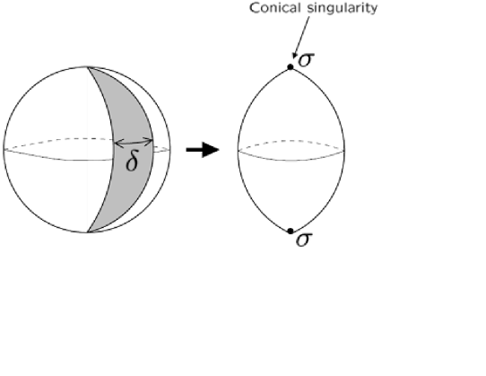
Figure 1.3: The rugby ball geometry with two branes of tension $\sigma$ at the conical singularities.

Now, we can easily see that the 4D geometry is independent of the branes’ tension $\sigma$. The branes’ vacuum energy does not curve the 4D spacetime as it would in 4D general relativity. This property was called self-tuning. It does not solve the CC problem because we still need to tune the value of $B_{0}$, but this idea looks promising as it breaks the standard relation between the 4D vacuum energy and the curvature of the 4D spacetime. Also, if the self-tuning mechanism worked, it would push the value of the CC to zero but we would still have to find a way to generate a small CC to agree with observations.

There are several objections to the idea of self-tuning [32]. The simplest argument is as follows. Suppose that we have tuned the initial value of $B_{0}$ to $B_{0}^{2}=2\Lambda_{6}$ and suppose that the branes’ tension were to change from an initial value to a different final value. This would imply that the area of the extra-dimensions ($4\pi\alpha$) would change too, because $\alpha$ is a function of $\sigma$. On the other hand, the magnetic flux in the internal space has to be conserved, this necessarily implies that the final magnetic field strength cannot satisfy $B_{0final}^{2}=2\Lambda_{6}$. Therefore the 4D spacetime will no longer be a static Minkowski spacetime but rather a time-dependent spacetime.

1.6.2 Supersymmetric large extra-dimensions

In the previous subsection, we have seen that the failure of the self-tuning is directly related to the tuning of the magnetic field strength with the bulk CC, which is necessary to obtain 4D Minkowski spacetime. The so-called supersymmetric large extra-dimension (SLED) model was proposed to try to address this problem. For excellent review articles see [30, 33, 34].

The action of this model is similar to the action of the Einstein-Maxwell model with an additional field $\phi$, the dilaton, it reads

$$S=\int d^{6}x\sqrt{-{}^{(6)}\!\!g}\left[\frac{M^{4}_{6}}{2}\left({}^{(6)}\!\!R-\partial_{a}\phi\partial^{a}\phi\right)-e^{\phi}\Lambda_{6}-\frac{1}{4}e^{-\phi}F_{ab}F^{ab}\right].$$ (1.72)

Comparing this model with the Einstein-Maxwell model it is easy to see that there exists a solution with $\phi=\phi_{0}$, where $\phi_{0}$ is a constant. It is also a solution of the Einstein-Maxwell model with the rescalings $\Lambda_{6}\rightarrow\Lambda_{6}e^{-\phi}$, $B_{0}^{2}\rightarrow B_{0}^{2}e^{\phi}$, provided that $\phi$ is at the minimum of its potential

$$V^{\prime}(\phi_{0})=-\frac{1}{2}B_{0}^{2}e^{-\phi_{0}}+\Lambda_{6}e^{\phi}=0.$$ (1.73)

This is the condition to have a flat geometry on the brane $B_{0}^{2}e^{-\phi_{0}}=2\Lambda_{6}e^{\phi}$. In other words, at the minimum, the vacuum energy is zero and therefore the geometry is Minkowski, this was called self-tuning.

As before, there are several objections to the idea of self-tuning, for example, Refs. [32, 35] derived the 4D effective theory using the metric ansatz

$$ds^{2}=g_{\mu\nu}(x)dx^{\mu}dx^{\nu}+M_{6}^{-2}e^{-2\psi(x)}\left(dr^{2}+\mathrm{sin}^{2}rd\theta^{2}\right),$$ (1.74)

and $\phi=\phi(x)$. The 4D effective potential is found to be

$$V(\psi,\phi)=M_{6}^{-4}e^{\sigma_{2}}U(\sigma_{1}),\quad U(\sigma_{1})=\frac{B_{0}^{2}}{2\alpha^{2}}e^{-2\sigma_{1}}-2M_{6}^{2}e^{-\sigma_{1}}+2\Lambda_{6},$$ (1.75)

where $\sigma_{1}=2\psi+\phi$, $\sigma_{2}=2\psi-\phi$ and $\alpha$ is related to the branes’ tension as $\alpha=1-\frac{\sigma}{2\pi M_{6}^{2}}$. They argued that if we start with a configuration in which $V(\psi,\phi)=0$, and if we change the branes’ tension to a different final value then $V(\psi,\phi)$ will be different from zero and $\sigma_{2}$ will have a runaway potential. The 4D spacetime becomes non-static.

This argument against self-tuning has raised criticisms [35]. For example, it is argued that the metric ansatz (1.74) is restrictive. There is a known class of static solutions with warping in the bulk that cannot be described by this ansatz. These solutions might play a role if self-tuning is to work. Chapter 3 is dedicated to the study of some aspects of this model and we shall derive the low energy effective theory including warping.

1.7 Warped compactifications in Type IIB supergravity

In chapter 4, we will present a method to obtain the 4D effective theory for warped compactifications including fluxes and branes in the 10D type IIB supergravity. In this section we shall introduce the general idea of warped compactification in type IIB supergravity (sugra). For further details about type IIB sugra we refer the reader to chapter 4 or to the extensive literature on the subject [36, 37, 38] and references therein.

The desire of embedding the Randall and Sundrum (RS) solution to the hierarchy problem in a string theory compactification was fulfilled with the work of Giddings, Kachru and Polchinski (GKP) [13]. They realized that a warped string compactification can generate a large hierarchy between the electroweak scale and the Planck scale in a similar way to the RS model [4]. To generate the warping of the extra-dimensions they needed to use not only positive tension objects like $D3$ branes but also negative tension objects. Figure 1.4 is a schematic representation of their model.

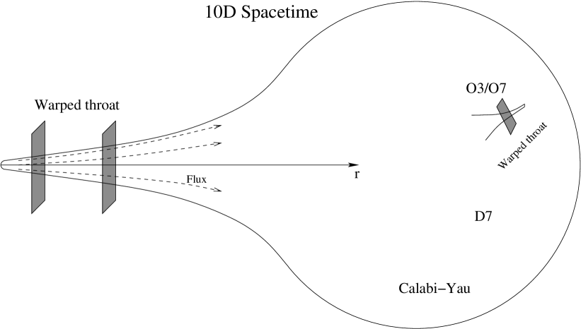
Figure 1.4: A warped throat compactification.

They start with a 10D spacetime, with six of the dimensions compactified in a Calabi-Yau manifold. In some region of the internal space, a throat develops. Fluxes and branes curve this space, giving origin to a warp factor $h(y)$. Their solution for the metric is

$$ds^{2}_{10}=h^{-\frac{1}{2}}(y)\eta_{\mu\nu}dx^{\mu}dx^{\nu}+h^{\frac{1}{2}}(y)\gamma_{mn}(y)dy^{m}dy^{n},$$ (1.76)

where $\gamma_{mn}$ and $y^{m}$ denote a Calabi-Yau metric and the coordinates of the extra-dimensions respectively. $x^{\mu}$ denotes the four-dimensional coordinates. The throat region of the spacetime is given by the solution found by Klebanov and Strassler [39] and it is well approximated by a 5D anti-de-Sitter spacetime with the remaining five extra-dimensions compactified in a small 5-sphere. In this region the RS mechanism of solving the hierarchy problem works as before.

These warped compactifications also provide models of inflation, where the inflaton is identified with the position of a brane in the extra-dimension $r$, where $r$ is a radial direction and it corresponds to one of the $y^{m}$. Brane-inflation models will be discussed in the chapter 5.

Chapter 2 Moduli instability in warped compactification

2.1 Introduction

The idea of using the degrees of freedom of extra spatial dimensions to unify gravity and the other interactions has attracted much interest. Especially, M-Theory has the potential to achieve this ultimate goal. Hořava and Witten showed that M-Theory compactified as $S^{1}/Z_{2}\times M^{10}$ reduces to a known string theory ($E_{8}\times E_{8}$ Heterotic String) [2]. From a low energy effective theory point of view, this model has a 5D spacetime (the bulk) with two 4D boundary hypersurfaces (the branes) [3]. The remaining six spatial dimensions are assumed to be compactified. All the Standard Model particles are confined to the branes while gravity can propagate in the bulk. As a consequence of the compactification of the six spatial dimensions, a 5D effective scalar field appears in the bulk, which describes the volume of the compactified 6D space.

A novel aspect of this model is that the fifth dimension is not homogeneous. The line element for a static solution is given in the form $ds_{5}^{2}=h^{\alpha}(r)dr^{2}+h^{\beta}(r)ds_{4}^{2}(x)$, where $r$ is the fifth coordinate, $\alpha$, $\beta$ are constants and $h$ is called the warp factor. In the previous chapter, we showed how this warped geometry was used by Randall and Sundrum [5] to address the hierarchy problem. They have also showed that it is possible to localize gravity around the brane with the warped geometry, providing in this way an alternative to compactification [4].

A new class of dynamical solutions that describes an instability of the warped geometry has been found. Chen et al. noticed that it is possible to obtain a dynamical solution by replacing the constant modulus in the warp factor $h$ by a linear function of the 4D coordinates [29]. This solution describes an instability of the model as the brane will hit the singularity in the bulk, where $h=0$. This kind of solution exists also in the 10D type IIB supergravity [40].

In this chapter, we study the moduli instability in a dilatonic two brane model, where the potentials for the scalar field on the brane and in the bulk obey the Bogomol’nyi-Prasad-Sommerfield (BPS) condition [41]. For particular values of parameters we retrieve either the Hořava-Witten theory or the Randall-Sundrum model. We identify the origin of the moduli instability using a 4D effective theory derived in Ref. [25] (see Refs. [42] and [43] for different approaches). This effective theory is derived by solving the 5D equations of motion using the gradient expansion method [12, 44, 45], where we assume that the velocities of the branes are small compared with the curvature scale of the bulk determined by the warp factor.

Despite the fact that the 4D effective theory is based on a slow-motion approximation, we will show that the 5D exact solutions can be reproduced in the 4D effective theory. In order to understand the relation between 4D solutions in an effective theory and full 5D solutions, we revisit the gradient expansion method by employing a new metric ansatz. Using this metric ansatz, we can clearly see why the moduli instability solution in the 4D effective theory can be lifted to an exact 5D solution.

We also comment on a claim that the 4D effective theory allows a much wider class of solutions than the 5D theory [46]. We disagree with that conclusion and we show that it is based on the restricted form of the 5D metric ansatz used in Ref. [46]. Using our metric ansatz, we provide a way to lift solutions in the 4D effective theory to 5D solutions perturbatively in terms of small velocities of the branes.

The structure of this chapter is as follows. In section 2.2, the model under consideration is described in detail. In section 2.3, we identify the solution in the 4D effective theory that describes the moduli instability. In section 2.4, we revisit the gradient expansion method to derive the 4D effective theory. We propose a new metric ansatz which is useful to relate 4D solutions in the effective theory to 5D solutions. Using this formalism we explain why the 4D solution for the moduli instability can be lifted to an exact 5D solution. In section 2.5, we comment on the arguments against the 4D effective theory. Section 2.6 is devoted to conclusions.

2.2 The model

Our model consists of a 5D spacetime (bulk) filled with a scalar field. The fifth dimension is a compact space $S^{1}$ with a $Z_{2}$ symmetry (i.e. identification $r\rightarrow-r$) and will be parameterized by the coordinate $r$, $0\leq r\leq L$. The bulk action takes the form

$$S_{bulk}=\frac{1}{2\kappa_{G}^{2}}\int d^{5}x\sqrt{-g_{5}}\left[{}^{5}\!R-\nabla_{M}\varphi\nabla^{M}\varphi+V_{bulk}(\varphi)\right],$$ (2.1)

where $\kappa_{G}$ denotes the 5D gravitational constant. Throughout this work Latin indices can have values in $\{r,t,x,y,z\}$, while Greek indices do not include the extra dimension coordinate $r$. The scalar field potential will be

$$V_{bulk}(\varphi)=-\left(b^{2}-\frac{2}{3}\right)e^{-2\sqrt{2}b\varphi}\sigma^{2},$$ (2.2)

where $\sigma$ and $b$ are the remaining parameters of this model. We can retrieve either the Randall-Sundrum model ($b=0$) or the Hořava-Witten model ($b=1$) according to the value of $b$. The orbifold $S^{1}/Z_{2}$ has two fixed points, at $r=0$ and $r=L$, and we can put branes there. The branes’ action is

$$S_{branes}=S_{+}+S_{-},$$ (2.3)

where $S_{+}$ and $S_{-}$ are the positive and negative tension brane action, respectively. They are given by

$$S_{\pm}=\mp\frac{\sqrt{2}}{\kappa_{G}^{2}}\int d^{4}x\sqrt{-g_{4}}e^{-\sqrt{2}b\varphi}\sigma.$$ (2.4)

The action of our model is

$$S_{total}=S_{bulk}+S_{branes}.$$ (2.5)

A schematic picture of our model is shown in Fig. 2.1

Figure 2.1: The dilatonic brane-world universe

2.3 Exact solutions for moduli instability in 4D effective theory

2.3.1 The exact 5D solution

Exact static solutions for the equations of motion that result from (2.5) were obtained in [41]. An interesting dynamical solution was found by Chen et al. [29]. They noticed that if we add a linear function of time to the warp factor of the solution of [41], it would still be a solution of the equations of motion. Their exact 5D solution reads

$$dS_{5}^{2} = \left(h\tau-\frac{|r|}{l}\right)^{\frac{6b^{2}-2}{3b^{2}+1}}dr^{2}+\left(h\tau-\frac{|r|}{l}\right)^{\frac{2}{3b^{2}+1}}\eta_{\mu\nu}dx^{\mu}dx^{\nu},$$ (2.6)

$$\varphi = \frac{3\sqrt{2}b}{3b^{2}+1}\ln\left(h\tau-\frac{|r|}{l}\right),\quad l=\frac{3}{3b^{2}+1}\frac{\sqrt{2}}{\sigma},$$ (2.7)

where $h$ is an arbitrary constant.

From the above equations we can read the scale factor of the positive tension brane ($r=0$) as

$$a^{2}_{+}(\tau)=\left(h\tau\right)^{\frac{2}{3b^{2}+1}},$$ (2.8)

and the scalar field as

$$\varphi(r=0,\tau)=\frac{3\sqrt{2}b}{3b^{2}+1}\ln(h\tau).$$ (2.9)

Let us choose $h<0$ and $\tau<0$. In this case the proper distance between branes, the so-called radion, is decreasing according to

$$\mathcal{R}=\int_{0}^{L}\left(h\tau-\frac{r}{l}\right)^{\frac{3b^{2}-1}{3b^{2}+1}}dr=l\frac{3b^{2}+1}{6b^{2}}(h\tau)^{\frac{6b^{2}}{3b^{2}+1}}\left[1-\left(1-\frac{L/l}{h\tau}\right)^{\frac{6b^{2}}{3b^{2}+1}}\right].$$ (2.10)

When $\tau\rightarrow-\infty$, $\mathcal{R}\rightarrow L\left(h\tau\right)^{\frac{3b^{2}-1}{3b^{2}+1}}$ and for $\tau=L/hl$, $\mathcal{R}=l(3b^{2}+1)\left(L/l\right)^{\frac{6b^{2}}{3b^{2}+1}}/6b^{2}$. Before the two branes collide, a curvature singularity will appear in the negative tension brane ($r=L$) at $\tau=L/hl$. This singularity will move towards the positive tension brane and will reach it at $\tau=0$. This event represents the total annihilation of the spacetime.

It is useful to note that if we drop the modulus sign in (2.6), the bulk spacetime is a static black brane or black hole solution depending on $b$, see [29] for more details. If $b=1$, there is a timelike curvature singularity at $h\tau=|r|/l$. From the static bulk point of view, the two branes are moving in this static bulk and the negative tension brane first hits the singularity. Even if the bulk spacetime is static, the existence of the branes, which gives the modulus sign for $r$, makes the spacetime truly time dependent.

Moduli instability is a serious problem for these types of model. In this work, we will try to understand it from a 4D effective theory viewpoint.

2.3.2 The exact solutions in 4D effective theory

In [25], Kobayashi and Koyama applied the gradient expansion method to solve perturbatively the 5D equations of motion resulting from (2.5). Their $0^{th}$ order solution reads

$$dS_{5}^{2} = d(t)^{2}e^{2\sqrt{2}b\phi(t)}dr^{2}+\mathcal{F}(r,t)^{\frac{1}{3b^{2}}}h_{\mu\nu}(t)dx^{\mu}dx^{\nu},$$ (2.11)

$$\varphi(r,t) = \frac{1}{\sqrt{2}b}\ln\mathcal{F}(r,t)+\phi(t),\quad\mathcal{F}(r,t)=1-\sqrt{2}b^{2}d(t)\sigma|r|.$$ (2.12)

The main result of the paper is a set of equations involving only four dimensional quantities that describe the dynamics of the unknown functions $d(t)$, $h_{\mu\nu}(t)$ and $\phi(t)$, appearing in Eqs. (2.11) and (2.12). It can be shown that their dynamical equations can be consistently deduced from the following action

$$S_{eff}=\frac{l}{2\kappa_{G}^{2}}\int d^{4}x\sqrt{-h}e^{\sqrt{2}b\phi}\left[\psi R(h)-\frac{3}{2(1+3b^{2})}\frac{1}{1-\psi}\nabla_{\alpha}\psi\nabla^{\alpha}\psi-\psi\nabla_{\alpha}\phi\nabla^{\alpha}\phi\right],$$ (2.13)

where here $\nabla_{\alpha}$ means the covariant derivative with respect to $h_{\mu\nu}$ and $\psi=1-\left(1-d\right)^{\frac{3b^{2}+1}{3b^{2}}}$. This is the action we obtain if we substitute Eqs. (2.11) and (2.12) into (2.5) and integrate over the extra dimension [42].

Performing the conformal transformation $h_{\mu\nu}=e^{-\sqrt{2}b\phi}f_{\mu\nu}/\psi$ and defining new scalar fields as

$$\psi=1-\tanh^{2}\left[\sqrt{\frac{1+3b^{2}}{6}}\Psi\right],$$ (2.14)

$$\phi=\frac{\Theta}{\sqrt{1+3b^{2}}}+\lambda\ln\psi,\quad\lambda\equiv-\frac{3}{\sqrt{2}}\frac{b}{3b^{2}+1},$$ (2.15)

we arrive at the action in the Einstein frame

$$S_{E}=\frac{l}{2\kappa_{G}^{2}}\int d^{4}x\sqrt{-f}\left[R(f)-\Theta_{|\alpha}\Theta^{|\alpha}-\Psi_{|\alpha}\Psi^{|\alpha}\right].$$ (2.16)

It is clear that the moduli fields have no potential and this is the origin of the instability. We are interested in cosmological solutions so we choose $f_{\mu\nu}$ to be a flat FRW metric. The Einstein equations resulting from the action (2.16) are

$$\frac{a^{\prime\prime}}{a}=-\frac{1}{6}\left({\Psi^{\prime}}^{2}+{\Theta^{\prime}}^{2}\right),\quad\left(\frac{a^{\prime}}{a}\right)^{2}=\frac{1}{6}\left({\Psi^{\prime}}^{2}+{\Theta^{\prime}}^{2}\right).$$ (2.17)

and the equations of motion for the scalar fields are

$$\Psi^{\prime\prime}+2\frac{a^{\prime}}{a}\Psi^{\prime}=0,\quad\Theta^{\prime\prime}+2\frac{a^{\prime}}{a}\Theta^{\prime}=0,$$ (2.18)

where $a(\tau)$ is the FRW scale factor and the prime denotes derivative with respect to the conformal time $\tau$. Equations (2.17,2.18) can be easily integrated to find

$$\Psi(\tau)=\sqrt{\frac{6}{3b^{2}+1}}\alpha\ln a^{2}+\gamma,\quad\Theta(\tau)=\sqrt{1+3b^{2}}\beta\ln a^{2}+\delta,\quad a^{2}(\tau)=\xi\tau+\zeta,$$ (2.19)

$$\alpha^{2}+\frac{(1+3b^{2})^{2}}{6}\beta^{2}=1+3b^{2},$$ (2.20)

where $\alpha$, $\beta$, $\gamma$, $\delta$, $\zeta$ and $\xi$ are integration constants. The solutions for the fields in the original frame can be obtained as

$$d(\tau)=1-\left[\frac{(\mu\tau+\nu)^{2\alpha}-1}{(\mu\tau+\nu)^{2\alpha}+1}\right]^{\frac{6b^{2}}{3b^{2}+1}},$$ (2.21)

$$\phi(\tau)=\ln\left[\frac{(\mu\tau+\nu)^{2\alpha\lambda(b)+\beta}}{\left[(\mu\tau+\nu)^{2\alpha}+1\right]^{2\lambda(b)}}\right]+\varrho,$$ (2.22)

where $\lambda(b)$ is defined in Eq. (2.15) and integration constants $\mu$, $\nu$, $\varrho$ are redefined from $\xi$, $\zeta$, $\gamma$ and $\delta$. The radion is calculated as

$$\mathcal{R}(\tau)=\frac{1}{\sqrt{2}b^{2}\sigma}d(\tau)e^{\sqrt{2}b\phi(\tau)},$$ (2.23)

and the square of the scale factor on the positive tension brane is

$$a^{2}_{+}(\tau)=\frac{e^{-\sqrt{2}b\phi(\tau)}}{\psi(\tau)}a^{2}(\tau).$$ (2.24)

We have found the remarkable fact that for a particular choice of the integration constants we can reproduce the exact solution found by Chen et al. described in the previous section. If we choose integration constants obeying the relations

$$\alpha=\frac{1}{2},\;\;\beta=-\lambda(b),\;\;\mu=\frac{2hl}{L},\;\;\nu=-1,$$ (2.25)

we get the same 4D quantities (scale factor and scalar field on the positive tension brane) and radion as the Chen et al. solution, Eqs. (2.8, 2.9, 2.10).

For this solution, the scale factor in the Einstein frame is given by

$$a^{2}(\tau)=\frac{2L}{l}\left(h\tau-\frac{L}{2l}\right).$$ (2.26)

If we take $h<0$, $\tau<0$, this corresponds to a collapsing universe, due to the kinetic energy of the scalar fields. At $\tau=L/2hl<0$, the universe in the Einstein frame reaches the Big-bang singularity. However, we should be careful to interpret this singularity. In fact, in the original 5D theory, $\tau=L/2hl$ does not correspond to any kind of singularity. In 5D theory, the negative tension brane hits the singularity at $\tau=L/hl$ and the positive tension brane hits the singularity at $\tau=0$. In fact at $\tau=L/2hl$, $\psi=0$ and so the conformal transformation becomes singular and the Einstein frame metric loses physical meaning.

2.4 Gradient expansion method with a new metric ansatz

In the previous section, we found that the exact solution derived in [29] can be reproduced from the $0^{th}$ order of the perturbative method. In this section, we will revisit the gradient expansion method which is used to derive the effective theory to clarify the reason why the exact solution derived in [29] can be reproduced within the 4D effective theory.

2.4.1 5D Equations

In this subsection we study the 5D equations of motion. From the action (2.5) we derive the Einstein’s equations

$${}^{5}G_{AB} = \nabla_{A}\varphi\nabla_{B}\varphi+\frac{1}{2}g_{AB}\left[-\nabla^{C}\varphi\nabla_{C}\varphi+V_{bulk}(\varphi)\right]$$

$$+\sqrt{2}\sigma\left[-\frac{\sqrt{g_{4}}}{\sqrt{g_{5}}}g_{\mu\nu}\delta_{A}^{\mu}\delta_{B}^{\nu}e^{-\sqrt{2}b\varphi}\delta(r)+\frac{\sqrt{g_{4}}}{\sqrt{g_{5}}}g_{\mu\nu}\delta_{A}^{\mu}\delta_{B}^{\nu}e^{-\sqrt{2}b\varphi}\delta(r-L)\right].$$

Assuming that the 5D line element has the form

$$dS_{5}^{2}=g_{AB}(X)dX^{A}dX^{B}=g_{rr}(x,r)dr^{2}+g_{\mu\nu}(x,r)dx^{\mu}dx^{\nu},$$ (2.28)

($x$ dependence means dependence of all the other coordinates $\{x,y,z,t\}$, except the extra dimension $r$) we can extract the junction conditions for the metric tensor from Einstein’s equation,

$$\sqrt{g^{rr}}\left(K_{\nu}^{\mu}-\delta_{\nu}^{\mu}K\right){\!}\Bigg{|}_{\stackrel{{\scriptstyle\scriptstyle{r=0^{+}}}}{{\scriptstyle{r=L^{-}}}}}=\mp\frac{1}{\sqrt{2}}\sigma e^{-\sqrt{2}b\varphi}\delta_{\nu}^{\mu}\Bigg{|}_{\stackrel{{\scriptstyle\scriptstyle{r=0^{+}}}}{{\scriptstyle{r=L^{-}}}}},$$ (2.29)

where the extrinsic curvature $K_{\mu\nu}$ is defined by $K_{\mu\nu}=-\frac{1}{2}\partial_{r}g_{\mu\nu}$. The scalar field equation of motion is

$$\Box\varphi+\sqrt{2}b\left(b^{2}-\frac{2}{3}\right)\sigma^{2}e^{-2\sqrt{2}b\varphi}=-2b\sigma\left[\sqrt{g^{rr}}e^{-\sqrt{2}b\varphi}\delta(r)-\sqrt{g^{rr}}e^{-\sqrt{2}b\varphi}\delta(r-L)\right],$$ (2.30)

and so the junction conditions for the scalar field are

$$\sqrt{g^{rr}}\partial_{r}\varphi{\!}\Bigg{|}_{\stackrel{{\scriptstyle\scriptstyle{r=0^{+}}}}{{\scriptstyle{r=L^{-}}}}}=\mp b\sigma e^{-\sqrt{2}b\varphi}\Bigg{|}_{\stackrel{{\scriptstyle\scriptstyle{r=0^{+}}}}{{\scriptstyle{r=L^{-}}}}}.$$ (2.31)

In order to proceed we shall assume that the 5D line element has further symmetries, described by

$$dS_{5}^{2}=e^{2\sqrt{2}b\tilde{\varphi}(x,r)}H^{\frac{6b^{2}-2}{3b^{2}+1}}(x,r)dr^{2}+H^{\frac{2}{3b^{2}+1}}(x,r)\tilde{g}_{\mu\nu}dx^{\mu}dx^{\nu},\quad H(x,r)=C(x)-\frac{r}{l}.$$ (2.32)

In this section, we will assume that the position of the second brane is $r=L=l$. For the scalar field we will assume the form

$$\varphi(x,r)=\frac{3\sqrt{2}b}{3b^{2}+1}\ln H+\tilde{\varphi}(x,r).$$ (2.33)

This metric ansatz is inspired by the time dependent solution (2.6,2.7) of Chen et al. [29]. Their solution was found by replacing the modulus parameter in the static solution by a linear function of time. In the same manner, we introduce an $x$ dependence in $H$ through the modulus parameter $C(x)$ in a covariant way . We also introduce the function $\tilde{\varphi}$ for the scalar field moduli. In order to satisfy the junction conditions (2.31) we must have the exponential factor in the $g_{rr}$ metric component. The tensor $\tilde{g}_{\mu\nu}$ is left completely general.

After some mathematical manipulations of the Einstein equations we obtain

$$\frac{1}{l}e^{-2\sqrt{2}b\tilde{\varphi}}H^{\frac{-9b^{2}+1}{3b^{2}+1}}\left(\frac{3b^{2}-5}{3b^{2}+1}\tilde{K}^{\mu}_{\nu}-\frac{1}{3b^{2}+1}\delta^{\mu}_{\nu}\tilde{K}\right)$$

$$-\sqrt{2}be^{-2\sqrt{2}b\tilde{\varphi}}H^{\frac{-3b^{2}+1}{3b^{2}+1}}\tilde{\varphi}_{,r}\left(\frac{1/l}{3b^{2}+1}H^{\frac{-6b^{2}}{3b^{2}+1}}\delta^{\mu}_{\nu}+H^{\frac{-3b^{2}+1}{3b^{2}+1}}\tilde{K}^{\mu}_{\nu}\right)$$

$$-H^{\frac{-3b^{2}-3}{3b^{2}+1}}\left(C_{|\nu}^{|\mu}+\frac{1}{3b^{2}+1}C_{|\alpha}^{|\alpha}\delta_{\nu}^{\mu}\right)-H^{-\frac{2}{3b^{2}+1}}\left[\sqrt{2}b\tilde{\varphi}_{|\nu}^{|\mu}+\left(2b^{2}+1\right)\tilde{\varphi}^{|\mu}\tilde{\varphi}_{|\nu}\right]$$

$$-\frac{\sqrt{2}b}{3b^{2}+1}H^{\frac{-3b^{2}-3}{3b^{2}+1}}\left[\left(3b^{2}+1\right)\left(\tilde{\varphi}^{|\mu}C_{|\nu}+\tilde{\varphi}_{|\nu}C^{|\mu}\right)+\tilde{\varphi}^{|\alpha}C_{|\alpha}\delta_{\nu}^{\mu}\right]$$

$$+e^{-2\sqrt{2}b\tilde{\varphi}}H^{\frac{-6b^{2}+2}{3b^{2}+1}}\left(\tilde{K}^{\mu}_{\nu,r}-\tilde{K}\tilde{K}^{\mu}_{\nu}\right)+H^{-\frac{2}{3b^{2}+1}}R_{\nu}^{\mu}(\tilde{g})=0,$$ (2.34)

$$\frac{1}{l}\frac{3b^{2}-3}{3b^{2}+1}e^{-2\sqrt{2}b\tilde{\varphi}}H^{\frac{-9b^{2}+1}{3b^{2}+1}}\tilde{K}+e^{-2\sqrt{2}b\tilde{\varphi}}H^{\frac{-6b^{2}+2}{3b^{2}+1}}\left(\tilde{K}_{,r}-\tilde{K}^{\alpha\beta}\tilde{K}_{\alpha\beta}\right)$$

$$+e^{-2\sqrt{2}b\tilde{\varphi}}H^{\frac{-6b^{2}+2}{3b^{2}+1}}\tilde{\varphi}_{,r}\left(\frac{1}{l}\frac{2\sqrt{2}b}{3b^{2}+1}H^{-1}-\sqrt{2}b\tilde{K}-\tilde{\varphi}_{,r}\right)$$

$$-H^{\frac{-3b^{2}-3}{3b^{2}+1}}\left(\frac{3b^{2}-1}{3b^{2}+1}C_{|\alpha}^{|\alpha}+\frac{6\sqrt{2}b^{3}}{3b^{2}+1}\tilde{\varphi}^{|\alpha}C_{|\alpha}\right)$$

$$-\sqrt{2}bH^{-\frac{2}{3b^{2}+1}}\left(\tilde{\varphi}_{|\alpha}^{|\alpha}+\sqrt{2}b\tilde{\varphi}^{|\alpha}\tilde{\varphi}_{|\alpha}\right)=0,$$ (2.35)

$$\tilde{K}^{\alpha}_{\beta|\alpha}-\tilde{K}_{|\beta}+\sqrt{2}b\left(\tilde{\varphi}_{|\beta}\tilde{K}-\tilde{\varphi}_{|\alpha}\tilde{K}^{\alpha}_{\beta}\right)+H^{-1}\left(\frac{3b^{2}-2}{3b^{2}+1}C_{|\beta}\tilde{K}-\frac{3b^{2}-5}{3b^{2}+1}C_{|\alpha}\tilde{K}^{\alpha}_{\beta}\right)$$

$$=-\tilde{\varphi}_{,r}\left(\frac{3\sqrt{2}b}{3b^{2}+1}H^{-1}C_{|\beta}+\tilde{\varphi}_{|\beta}\right),$$ (2.36)

where $\tilde{K}_{\mu\nu}$ is defined like $\tilde{K}_{\mu\nu}=-\frac{1}{2}\partial_{r}{\tilde{g}_{\mu\nu}}$, $\tilde{K}$ is the trace of $\tilde{K}_{\mu\nu}$, $\scriptstyle{|}_{\scriptstyle{\alpha}}$ denotes covariant derivative with respect to $\tilde{g}_{\mu\nu}$ and $R_{\mu\nu}(\tilde{g})$ is the Ricci tensor of $\tilde{g}_{\mu\nu}$. Equation (2.30) transforms into

$$\!\!\!\!\!\!\!\!\!e^{-2\sqrt{2}b\tilde{\varphi}}H^{\frac{-3b^{2}+5}{3b^{2}+1}}\bigg{[}\tilde{\varphi}_{,rr}-\sqrt{2}b\left(\tilde{\varphi}_{,r}\right)^{2}-\tilde{\varphi}_{,r}\tilde{K}+\frac{1}{l}\frac{3\sqrt{2}b}{3b^{2}+1}H^{-1}\tilde{K}+\frac{1}{l}\frac{9b^{2}-5}{3b^{2}+1}H^{-1}\tilde{\varphi}_{,r}\bigg{]}$$

$$\!\!\!\!\!\!\!\!\!+H\tilde{\varphi}_{|\alpha}^{|\alpha}+\frac{3\sqrt{2}b}{3b^{2}+1}C_{|\alpha}^{|\alpha}+\sqrt{2}bH\tilde{\varphi}_{|\alpha}\tilde{\varphi}^{|\alpha}+\frac{9b^{2}+1}{3b^{2}+1}\tilde{\varphi}_{|\alpha}C^{|\alpha}=0.$$ (2.37)

With this particular ansatz the junction conditions (2.29,2.31) are significantly simplified and read

$$\left[\tilde{K}_{\nu}^{\mu}\right]{\!}\Bigg{|}_{\stackrel{{\scriptstyle\scriptstyle{r=0^{+}}}}{{\scriptstyle{r=l^{-}}}}}=0,$$ (2.38)

$$\left[\tilde{\varphi}_{,r}\right]{\!}\Bigg{|}_{\stackrel{{\scriptstyle\scriptstyle{r=0^{+}}}}{{\scriptstyle{r=l^{-}}}}}=0.$$ (2.39)

It is impossible to solve these equations in general, so in the next section, we will solve them using the gradient expansion method up to first order in the perturbations.

2.4.2 The gradient expansion

The approximation

In order to use perturbation theory to solve a system of differential equations we need to identify the characteristic scale of the different terms involved in the equations and then see if there is a small parameter.

The derivatives along the extra dimension of the conformal metric $\tilde{g}_{\mu\nu}$ as well as the derivative of $\tilde{\varphi}$ are of order $1/l$. Typically, we take $l$ to be of order of a few tenths of a millimeter. If the characteristic brane’s curvature length scale is $D$ then $\partial^{2}_{x}\,\tilde{g}_{\mu\nu}\sim 1/D^{2}\tilde{g}_{\mu\nu}$. We assume that variations along the branes’ coordinates are small in comparison with $1/l$. This implies that the radion changes slowly or that the speed of the branes is small. More precisely, our small parameters will be

$$l^{2}\partial^{2}_{x}(\ldots)\ll 1\;\;\;\;\;\mbox{and}\;\;\;\;\;\left(l\partial_{x}\ldots\right)^{2}\ll 1,$$ (2.40)

where $\ldots$ represents the conformal metric functions, $C$ or $\tilde{\varphi}$.

As in the usual perturbation method, we expand the unknown functions in a series

$$\tilde{g}_{\mu\nu}(r,x)=\stackrel{{\scriptstyle(0)}}{{\tilde{g}}}_{\mu\nu}(r,x)+\stackrel{{\scriptstyle(1)}}{{\tilde{g}}}_{\mu\nu}(r,x)+\cdots,$$ (2.41)

$$\tilde{\varphi}(r,x)=\stackrel{{\scriptstyle(0)}}{{\tilde{\varphi}}}(r,x)+\stackrel{{\scriptstyle(1)}}{{\tilde{\varphi}}}(r,x)+\cdots.$$ (2.42)

We impose the boundary conditions at the position of the positive tension brane

$$\stackrel{{\scriptstyle(n)}}{{\tilde{g}}}_{\mu\nu}(r=0,x)=0,\;\mbox{for all}\;n>0,$$ (2.43)

$$\stackrel{{\scriptstyle(n)}}{{\tilde{\varphi}}}(r=0,x)=0,\;\mbox{for all}\;n>0.$$ (2.44)

Other quantities are naturally expanded as

$$\tilde{K}_{\mu\nu}=\stackrel{{\scriptstyle(0)}}{{\tilde{K}}}_{\mu\nu}+\stackrel{{\scriptstyle(1)}}{{\tilde{K}}}_{\mu\nu}+\cdots.$$ (2.45)

In practical terms, at zeroth order in the gradient expansion method we ignore all derivatives along the branes’ coordinates. These terms will only enter the first order equations. At zeroth order, the 5D partial differential equations of motion reduce to simpler ordinary differential equations on the extra dimension coordinate. The gradient expansion method has also been used in the 4D cosmological context [47, 48, 49, 50, 51].

$0^{th}$ Order (Background geometry)

The $0^{th}$ order system can be easily integrated with respect to the extra dimension coordinate $r$ to get the particular solution

$$\stackrel{{\scriptstyle(0)}}{{\tilde{g}_{\mu\nu}}}(r,x)=\stackrel{{\scriptstyle(0)}}{{\tilde{g}_{\mu\nu}}}(x),$$ (2.46)

$$\stackrel{{\scriptstyle(0)}}{{\tilde{\varphi}}}(r,x)=\stackrel{{\scriptstyle(0)}}{{\tilde{\varphi}}}(x).$$ (2.47)

This solution clearly satisfies the $0^{th}$order junction conditions.

$1^{st}$ Order

At $1^{st}$ order the evolution equations are

$$\!\!\!\!\!\!\!\!\!\!\!\!\!\!\!\!\!\!\frac{1}{l}e^{-2\sqrt{2}b\stackrel{{\scriptstyle(0)}}{{\tilde{\varphi}}}}H^{\frac{-9b^{2}+1}{3b^{2}+1}}\left(\frac{3b^{2}-5}{3b^{2}+1}\stackrel{{\scriptstyle(1)}}{{\tilde{K}^{\mu}_{\nu}}}-\frac{1}{3b^{2}+1}\delta^{\mu}_{\nu}\stackrel{{\scriptstyle(1)}}{{\tilde{K}}}\right)+e^{-2\sqrt{2}b\stackrel{{\scriptstyle(0)}}{{\tilde{\varphi}}}}H^{\frac{-6b^{2}+2}{3b^{2}+1}}\stackrel{{\scriptstyle(1)}}{{\tilde{K}^{\mu}_{\nu,r}}}$$

$$\!\!\!\!\!\!\!\!\!\!\!\!\!\!\!\!\!\!-H^{\frac{-3b^{2}-3}{3b^{2}+1}}\left(C_{|\nu}^{|\mu}+\frac{1}{3b^{2}+1}C_{|\alpha}^{|\alpha}\delta_{\nu}^{\mu}\right)-H^{-\frac{2}{3b^{2}+1}}\left[\sqrt{2}b\stackrel{{\scriptstyle(0)}}{{\tilde{\varphi}_{|\nu}^{|\mu}}}+\left(2b^{2}+1\right)\stackrel{{\scriptstyle(0)}}{{\tilde{\varphi}^{|\mu}}}\stackrel{{\scriptstyle(0)}}{{\tilde{\varphi}_{|\nu}}}\right]$$

$$\!\!\!\!\!\!\!\!\!\!\!\!\!\!\!\!\!\!-\frac{\sqrt{2}b}{3b^{2}+1}H^{\frac{-3b^{2}-3}{3b^{2}+1}}\left[\left(3b^{2}+1\right)\left(\stackrel{{\scriptstyle(0)}}{{\tilde{\varphi}^{|\mu}}}C_{|\nu}+\stackrel{{\scriptstyle(0)}}{{\tilde{\varphi}_{|\nu}}}C^{|\mu}\right)+\stackrel{{\scriptstyle(0)}}{{\tilde{\varphi}^{|\alpha}}}C_{|\alpha}\delta_{\nu}^{\mu}\right]$$

$$\!\!\!\!\!\!\!\!\!\!\!\!\!\!\!\!\!\!-\frac{\sqrt{2}b}{l}\frac{1}{3b^{2}+1}e^{-2\sqrt{2}b\stackrel{{\scriptstyle(0)}}{{\tilde{\varphi}}}}H^{\frac{-9b^{2}+1}{3b^{2}+1}}\stackrel{{\scriptstyle(1)}}{{\tilde{\varphi}_{,r}}}\delta^{\mu}_{\nu}+H^{-\frac{2}{3b^{2}+1}}R_{\nu}^{\mu}\left(\stackrel{{\scriptstyle(0)}}{{\tilde{g}}}\right)=0,$$ (2.48)

$$\!\!\!\!\!\!\!\!\!\!\!\!\!\!\!\!\!\!\frac{1}{l}\frac{3b^{2}-3}{3b^{2}+1}e^{-2\sqrt{2}b\stackrel{{\scriptstyle(0)}}{{\tilde{\varphi}}}}H^{\frac{-9b^{2}+1}{3b^{2}+1}}\stackrel{{\scriptstyle(1)}}{{\tilde{K}}}+e^{-2\sqrt{2}b\stackrel{{\scriptstyle(0)}}{{\tilde{\varphi}}}}H^{\frac{-6b^{2}+2}{3b^{2}+1}}\stackrel{{\scriptstyle(1)}}{{\tilde{K}_{,r}}}$$

$$\!\!\!\!\!\!\!\!\!\!\!\!\!\!\!\!\!\!-H^{\frac{-3b^{2}-3}{3b^{2}+1}}\left(\frac{3b^{2}-1}{3b^{2}+1}C_{|\alpha}^{|\alpha}+\frac{6\sqrt{2}b^{3}}{3b^{2}+1}\stackrel{{\scriptstyle(1)}}{{\tilde{\varphi}^{|\alpha}}}C_{|\alpha}\right)$$

$$\!\!\!\!\!\!\!\!\!\!\!\!\!\!\!\!\!\!+\frac{1}{l}\frac{2\sqrt{2}b}{3b^{2}+1}e^{-2\sqrt{2}b\stackrel{{\scriptstyle(0)}}{{\tilde{\varphi}}}}H^{\frac{-9b^{2}+1}{3b^{2}+1}}\stackrel{{\scriptstyle(1)}}{{\tilde{\varphi}_{,r}}}-\sqrt{2}bH^{-\frac{2}{3b^{2}+1}}\left(\stackrel{{\scriptstyle(0)}}{{\tilde{\varphi}_{|\alpha}^{|\alpha}}}+\sqrt{2}b\stackrel{{\scriptstyle(0)}}{{\tilde{\varphi}^{|\alpha}}}\stackrel{{\scriptstyle(0)}}{{\tilde{\varphi}_{|\alpha}}}\right)=0,$$ (2.49)

$$\!\!\!\!\!\!\!\!\!\!\!\!\!\!\!\!\!\!e^{-2\sqrt{2}b\stackrel{{\scriptstyle(0)}}{{\tilde{\varphi}}}}H^{\frac{-3b^{2}+5}{3b^{2}+1}}\left[\stackrel{{\scriptstyle(1)}}{{\tilde{\varphi}_{,rr}}}+\frac{1}{l}\frac{1}{3b^{2}+1}H^{-1}\left(3\sqrt{2}b\stackrel{{\scriptstyle(1)}}{{\tilde{K}}}+\left(9b^{2}-5\right)\stackrel{{\scriptstyle(1)}}{{\tilde{\varphi}_{,r}}}\right)\right]$$

$$\!\!\!\!\!\!\!\!\!\!\!\!\!\!\!\!\!\!+H\stackrel{{\scriptstyle(0)}}{{\tilde{\varphi}_{|\alpha}^{|\alpha}}}+\frac{3\sqrt{2}b}{3b^{2}+1}C_{|\alpha}^{|\alpha}+\sqrt{2}bH\stackrel{{\scriptstyle(0)}}{{\tilde{\varphi}_{|\alpha}}}\stackrel{{\scriptstyle(0)}}{{\tilde{\varphi}^{|\alpha}}}+\frac{9b^{2}+1}{3b^{2}+1}\stackrel{{\scriptstyle(0)}}{{\tilde{\varphi}_{|\alpha}}}C^{|\alpha}=0.$$ (2.50)

The junction conditions at this order are

$$\left[\stackrel{{\scriptstyle(1)}}{{\tilde{K}_{\nu}^{\mu}}}\right]{\!}\Bigg{|}_{\stackrel{{\scriptstyle\scriptstyle{r=0^{+}}}}{{\scriptstyle{r=l^{-}}}}}=0,$$ (2.51)

$$\left[\stackrel{{\scriptstyle(1)}}{{\tilde{\varphi}_{,r}}}\right]{\!}\Bigg{|}_{\stackrel{{\scriptstyle\scriptstyle{r=0^{+}}}}{{\scriptstyle{r=l^{-}}}}}=0.$$ (2.52)

In the preceding equations all the indices are raised with the zeroth order metric. Combining the trace of equation (2.48) with equation (2.49) we obtain

$$\frac{1}{l}e^{-2\sqrt{2}b\stackrel{{\scriptstyle(0)}}{{\tilde{\varphi}}}}\stackrel{{\scriptstyle(1)}}{{\tilde{K}}} = \frac{3b^{2}+1}{6}\left[R\left(\stackrel{{\scriptstyle(0)}}{{\tilde{g}}}\right)-\stackrel{{\scriptstyle(0)}}{{\tilde{\varphi}_{|\alpha}}}\stackrel{{\scriptstyle(0)}}{{\tilde{\varphi}^{|\alpha}}}\right]H^{\frac{9b^{2}-3}{3b^{2}+1}}-\frac{\sqrt{2}b}{l}e^{-2\sqrt{2}b\stackrel{{\scriptstyle(0)}}{{\tilde{\varphi}}}}\stackrel{{\scriptstyle(1)}}{{\tilde{\varphi}_{,r}}}$$ (2.53)

$$-\left(C_{|\alpha}^{|\alpha}+\sqrt{2}bC_{|\alpha}\stackrel{{\scriptstyle(0)}}{{\tilde{\varphi}^{|\alpha}}}\right)H^{\frac{6b^{2}-4}{3b^{2}+1}}.$$

Imposing the junction conditions (2.51,2.52) we get

$$\tilde{R}\left(\stackrel{{\scriptstyle(0)}}{{\tilde{g}}}\right)=\stackrel{{\scriptstyle(0)}}{{\tilde{\varphi}_{|\alpha}}}\stackrel{{\scriptstyle(0)}}{{\tilde{\varphi}^{|\alpha}}},$$ (2.54)

and the equation of motion for the 4D effective scalar field

$$C_{|\alpha}^{|\alpha}+\sqrt{2}bC_{|\alpha}\stackrel{{\scriptstyle(0)}}{{\tilde{\varphi}^{|\alpha}}}=0.$$ (2.55)

Equation (2.53) now reads

$$\stackrel{{\scriptstyle(1)}}{{\tilde{K}}}=-\sqrt{2}b\stackrel{{\scriptstyle(1)}}{{\tilde{\varphi}_{,r}}}.$$ (2.56)

Using the decomposition of $\stackrel{{\scriptstyle(1)}}{{\tilde{K_{\nu}^{\mu}}}}$ in

$$\stackrel{{\scriptstyle(1)}}{{\tilde{K_{\nu}^{\mu}}}}=\stackrel{{\scriptstyle(1)}}{{\tilde{\Sigma_{\nu}^{\mu}}}}+\frac{1}{4}\delta_{\nu}^{\mu}\stackrel{{\scriptstyle(1)}}{{\tilde{K}}},$$ (2.57)

equation (2.48) can be easily integrated to find

$$\!\!\!\!\!\!\!\!\!\!\!\!\!\!\!\!\!\!\!\!\!\!\!\!\!\!e^{-2\sqrt{2}b\stackrel{{\scriptstyle(0)}}{{\tilde{\varphi}}}}H^{-\frac{3b^{2}-5}{3b^{2}+1}}\stackrel{{\scriptstyle(1)}}{{\tilde{\Sigma_{\nu}^{\mu}}}}=\Bigg{[}\left(C_{|\nu}^{|\mu}+\sqrt{2}b\left(C_{|\nu}\stackrel{{\scriptstyle(0)}}{{\tilde{\varphi}^{|\mu}}}+C^{|\mu}\stackrel{{\scriptstyle(0)}}{{\tilde{\varphi}_{|\nu}}}\right)\right)r$$

$$\!\!\!\!\!\!\!\!\!\!\!\!\!\!\!\!\!\!\!\!\!\!\!\!\!\!-\left(R_{\nu}^{\mu}\left(\stackrel{{\scriptstyle(0)}}{{\tilde{g}}}\right)-\sqrt{2}b\stackrel{{\scriptstyle(0)}}{{\tilde{\varphi}_{|\nu}^{|\mu}}}-\left(2b^{2}+1\right)\stackrel{{\scriptstyle(0)}}{{\tilde{\varphi}_{|\nu}}}\stackrel{{\scriptstyle(0)}}{{\tilde{\varphi}^{|\mu}}}\right)\left(Cr-\frac{r^{2}}{2l}\right)\Bigg{]}_{traceless}+\chi_{\nu}^{\mu}(x),$$ (2.58)

where $\chi_{\nu}^{\mu}(x)$ is an integration constant and the subscript $[\;\;]_{traceless}$ means the traceless part of the quantity between square brackets. In terms of $\tilde{\Sigma_{\nu}^{\mu}}$, the junction conditions (2.51) are

$$\left[\stackrel{{\scriptstyle(1)}}{{\tilde{\Sigma}_{\nu}^{\mu}}}\right]{\!}\Bigg{|}_{\stackrel{{\scriptstyle\scriptstyle{r=0^{+}}}}{{\scriptstyle{r=l^{-}}}}}=0.$$ (2.59)

From the previous junction conditions (2.59) we can obtain the 4D effective equations of motion

$$\!\!\!\!\!\!\!\!\!\!\!\!\!\!\!\!\!\!\!\tilde{R}_{\nu}^{\mu}\left(\stackrel{{\scriptstyle(0)}}{{\tilde{g}}}\right) = \left(C-\frac{1}{2}\right)^{-1}\left[C_{|\nu}^{|\mu}+\frac{1}{4}\delta_{\nu}^{\mu}C_{|\alpha}^{|\alpha}+\sqrt{2}b\left(C_{|\nu}\stackrel{{\scriptstyle(0)}}{{\tilde{\varphi}^{|\mu}}}+C_{|\mu}\stackrel{{\scriptstyle(0)}}{{\tilde{\varphi}^{|\nu}}}\right)\right]$$ (2.60)

$$+\sqrt{2}b\left(\stackrel{{\scriptstyle(0)}}{{\tilde{\varphi}_{|\nu}^{|\mu}}}-\frac{1}{4}\delta_{\nu}^{\mu}\stackrel{{\scriptstyle(0)}}{{\tilde{\varphi}_{|\alpha}^{|\alpha}}}\right)+\left(2b^{2}+1\right)\stackrel{{\scriptstyle(0)}}{{\tilde{\varphi}_{|\nu}}}\stackrel{{\scriptstyle(0)}}{{\tilde{\varphi}^{|\mu}}}-\frac{b^{2}}{2}\delta_{\nu}^{\mu}\stackrel{{\scriptstyle(0)}}{{\tilde{\varphi}_{|\alpha}}}\stackrel{{\scriptstyle(0)}}{{\tilde{\varphi}^{|\alpha}}},$$

and

$$\chi_{\nu}^{\mu}(x)=0.$$ (2.61)

Combining equation (2.56) with the scalar field equation (2.50) and integrating it once with respect to the extra dimension, we get (after using the previous equations of motion to simplify the result)

$$e^{-2\sqrt{2}b\stackrel{{\scriptstyle(0)}}{{\tilde{\varphi}}}}H^{\frac{-3b^{2}+5}{3b^{2}+1}}\stackrel{{\scriptstyle(1)}}{{\tilde{\varphi}_{,r}}}=-\left(Cr-\frac{r^{2}}{2l}\right)\left(\stackrel{{\scriptstyle(0)}}{{\tilde{\varphi}_{|\alpha}^{|\alpha}}}+\sqrt{2}b\stackrel{{\scriptstyle(0)}}{{\tilde{\varphi}_{|\alpha}}}\stackrel{{\scriptstyle(0)}}{{\tilde{\varphi}^{|\alpha}}}\right)-\stackrel{{\scriptstyle(0)}}{{\tilde{\varphi}^{|\alpha}}}C_{|\alpha}r+\Xi(x),$$ (2.62)

where $\Xi(x)$ is just an integration constant.

The junction conditions (2.52) give

$$\Xi(x)=0$$ (2.63)

and the equation of motion for the second 4D effective scalar field

$$\stackrel{{\scriptstyle(0)}}{{\tilde{\varphi}_{|\alpha}^{|\alpha}}}+\sqrt{2}b\stackrel{{\scriptstyle(0)}}{{\tilde{\varphi}_{|\alpha}}}\stackrel{{\scriptstyle(0)}}{{\tilde{\varphi}^{|\alpha}}}=-\left(C-\frac{1}{2}\right)^{-1}\stackrel{{\scriptstyle(0)}}{{\tilde{\varphi}^{|\alpha}}}C_{|\alpha}.$$ (2.64)

2.4.3 The 4D Effective theory

The 4D effective equations of motion are summarized as

$$\!\!\!\!\!\!\!\!\!\!\!\!\!\!\!\!\!\!\!\tilde{R}_{\nu}^{\mu}\left(\stackrel{{\scriptstyle(0)}}{{\tilde{g}}}\right) = \left(C-\frac{1}{2}\right)^{-1}\left[C_{|\nu}^{|\mu}+\frac{1}{4}\delta_{\nu}^{\mu}C_{|\alpha}^{|\alpha}+\sqrt{2}b\left(C_{|\nu}\stackrel{{\scriptstyle(0)}}{{\tilde{\varphi}^{|\mu}}}+C_{|\mu}\stackrel{{\scriptstyle(0)}}{{\tilde{\varphi}^{|\nu}}}\right)\right]$$ (2.65)

$$+\sqrt{2}b\left(\stackrel{{\scriptstyle(0)}}{{\tilde{\varphi}_{|\nu}^{|\mu}}}-\frac{1}{4}\delta_{\nu}^{\mu}\stackrel{{\scriptstyle(0)}}{{\tilde{\varphi}_{|\alpha}^{|\alpha}}}\right)+\left(2b^{2}+1\right)\stackrel{{\scriptstyle(0)}}{{\tilde{\varphi}_{|\nu}}}\stackrel{{\scriptstyle(0)}}{{\tilde{\varphi}^{|\mu}}}-\frac{b^{2}}{2}\delta_{\nu}^{\mu}\stackrel{{\scriptstyle(0)}}{{\tilde{\varphi}_{|\alpha}}}\stackrel{{\scriptstyle(0)}}{{\tilde{\varphi}^{|\alpha}}},$$

$$C_{|\alpha}^{|\alpha}+\sqrt{2}bC_{|\alpha}\stackrel{{\scriptstyle(0)}}{{\tilde{\varphi}^{|\alpha}}}=0,$$ (2.66)

$$\stackrel{{\scriptstyle(0)}}{{\tilde{\varphi}_{|\alpha}^{|\alpha}}}+\sqrt{2}b\stackrel{{\scriptstyle(0)}}{{\tilde{\varphi}_{|\alpha}}}\stackrel{{\scriptstyle(0)}}{{\tilde{\varphi}^{|\alpha}}}=-\left(C-\frac{1}{2}\right)^{-1}\stackrel{{\scriptstyle(0)}}{{\tilde{\varphi}^{|\alpha}}}C_{|\alpha},$$ (2.67)

and they can be deduced from the following action

$$S_{eff}=\frac{l}{\kappa_{G}^{2}}\int d^{4}x\sqrt{-\stackrel{{\scriptstyle(0)}}{{\tilde{g}}}}\left(C-\frac{1}{2}\right)e^{\sqrt{2}b\stackrel{{\scriptstyle(0)}}{{\tilde{\varphi}}}}\left[R(\stackrel{{\scriptstyle(0)}}{{\tilde{g}}})-\stackrel{{\scriptstyle(0)}}{{\tilde{\varphi}_{|\alpha}}}\stackrel{{\scriptstyle(0)}}{{\tilde{\varphi}^{|\alpha}}}\right],$$ (2.68)

where $\scriptstyle{|}_{\scriptstyle{\alpha}}$ denotes covariant derivative with respect to $\stackrel{{\scriptstyle(0)}}{{\tilde{g}_{\mu\nu}}}$. We should note that this effective action can be derived by substituting in (2.5) the 5D solutions up to the first order and integrating it over the fifth dimension [43].

As a consistency check, we see that if we perform the conformal transformation

$$h_{\mu\nu}(x)=C^{\frac{2}{3b^{2}+1}}(x)\stackrel{{\scriptstyle(0)}}{{\tilde{g}_{\mu\nu}}}(x),$$ (2.69)

the previous action reduces to (2.13) if the effective scalar fields of the two theories are related through

$$\psi=2C^{-2}\left(C-\frac{1}{2}\right),$$ (2.70)

$$\phi(x)=\frac{3\sqrt{2}b}{3b^{2}+1}\ln C+\stackrel{{\scriptstyle(0)}}{{\tilde{\varphi}}}(x).$$ (2.71)

The check consists in seeing that these relations are exactly the ones required so that the two observables (the proper distance between branes and the scalar field on the positive tension brane) agree in both approaches.

2.4.4 The 5D exact solution

It is straightforward to find a cosmological solution of this 4D effective theory. For example we can easily find the following particular solution

$$\stackrel{{\scriptstyle(0)}}{{\tilde{g}_{\mu\nu}}}(x)=\eta_{\mu\nu},\quad C(x)=ht,\quad\stackrel{{\scriptstyle(0)}}{{\tilde{\varphi}}}(x)=0,$$ (2.72)

where $h$ is an integration constant.

Now we are ready to address the question why the above solution can be lifted to an exact 5D solution. Let us start by calculating the next order correction ${}^{(1)}{\tilde{g}_{\mu\nu}}$ and ${}^{(1)}{\tilde{\varphi}}$. Eq. (2.62) and the boundary conditions (2.44) give ${}^{(1)}{\tilde{\varphi}}=0$, if we take as $0^{th}$ order solution Eqs. (2.72). We can construct ${}^{(1)}{\tilde{K}_{\mu\nu}}$ from Eqs. (2.56) and (2.58). For the $0^{th}$ order solution (2.72) this gives ${}^{(1)}{\tilde{K}_{\mu\nu}}=0$. After imposing the boundary conditions (2.43), we obtain that the next order correction vanishes, ${}^{(1)}{\tilde{g}_{\mu\nu}(r,x)}=0$. For solution (2.72) it turns out that all the corrections vanish and the $0^{th}$ order solution is an exact solution of the non-perturbed 5D Eqs. (2.34-2.39).

For other solutions of the 4D effective theory, higher order corrections will not vanish and therefore they should be taken into account in the reconstruction of the 5D metric. Using the gradient expansion method, we can reconstruct the 5D solution perturbatively. We should emphasize that the choice of the $0^{th}$ order metric is quite important in order to reconstruct 5D solutions efficiently. Our metric ansatz has the advantage that it is possible to recover the exact solution of Chen et al. (2.72) at $0^{th}$ order. Indeed, if we had started with an ansatz like Eqs. (2.11,2.12) we would need an infinite number of higher order terms to obtain the exact 5D solution.

2.5 Validity of 4D effective theory

In this section we will make comments on a work by Kodama and Uzawa [46]. Let us start by briefly describing their arguments. After deriving the 4D effective theory for warped compactification of the 5D Hořava-Witten model (they also extend their analysis to 10D IIB supergravity and obtain the same conclusions), the authors show that the 4D effective theory allows a wider class of solutions than the fundamental higher dimensional theory. Therefore we should be careful in using this effective theory approach, because we may find 4D solutions that do not satisfy the equations of motion once lifted back to 5D.

The authors assume a metric ansatz of the form

$$dS_{5}^{2}=h(x,r)dr^{2}+h^{\frac{1}{2}}(x,r)\tilde{g}_{\mu\nu}(x)dx^{\mu}dx^{\nu},$$ (2.73)

where the warp factor has the form $h(x,r)=C(x)-r/L$. This corresponds to taking $\tilde{K}_{\mu\nu}=0$, $\tilde{\varphi}=0$ and $b=1$ (for the Hořava-Witten case) in our work. Then Eq. (2.34) reduces to

$$-H(r,x)^{-\frac{3}{2}}\left(C(x)_{|\nu}^{|\mu}+\frac{1}{4}C(x)_{|\alpha}^{|\alpha}\delta_{\nu}^{\mu}\right)+H(r,x)^{-\frac{1}{2}}R_{\nu}^{\mu}(\tilde{g}(x))=0.$$ (2.74)

In order to satisfy this equation for all values of $r$, we should have

$$R_{\mu\nu}(\tilde{g})=0,\quad C_{|\mu\nu}=0.$$ (2.75)

They obtain the 4D effective action, by integrating the fifth dimension, as

$$S_{eff}\propto\int d^{4}x\sqrt{-\tilde{g}}\left(C(x)-\frac{1}{2}\right)R(\tilde{g}),$$ (2.76)

which agrees with our effective action (2.68). As we have shown, this theory admits solutions with $R_{\mu\nu}(\tilde{g})\neq 0$ (see Eq. (2.65)), which do not obey the constraint (2.75) obtained from the 5D equations of motion.

However, it is clear from our analysis that their metric ansatz is too restrictive. If we consider a more general metric as our metric ansatz, we see that the 5D Einstein equations contain more terms given by $\tilde{K}_{\mu\nu}$. With the inclusion of these new terms, the 5D equations do not necessarily imply (2.75). Of course, the non-vanishing $\tilde{K}_{\mu\nu}$ changes the metric (2.73) and one could argue that the resultant 4D effective action would be also changed. However, it is shown that even if we include the first order corrections ${}^{(1)}{\tilde{g}_{\mu\nu}}(x)$ to the metric, the resultant 4D effective action derived by integrating out the fifth dimension does not change [43]. Therefore, for 4D solutions that do not satisfy (2.75), we should include the corrections to the metric (2.73). We have provided this correction perturbatively. Using Eqs. (2.53) and (2.58), we can reconstruct the correction to the metric, ${}^{(1)}{\tilde{g}_{\mu\nu}}(x)$, which is necessary to satisfy the 5D equation of motion.

We should emphasize that the validity of the 4D effective theory is based on the conditions (2.40). If the 4D effective theory admits a solution that violates the conditions (2.40), then there is no guarantee that the 4D solution can be lifted up to the 5D solution consistently. We should check the validity of the 4D effective theory by calculating the higher order corrections to ensure that the higher order corrections can be neglected consistently.

2.6 Conclusion

In this chapter, we have studied the moduli instability in a two brane model with a bulk scalar field found by Chen et al.. This model can be viewed as a generalization of the Hořava-Witten theory and the Randall-Sundrum model. The scalar field potentials in the bulk and on the branes are tuned in order to satisfy the BPS condition.

We used a low energy effective theory, which is derived by assuming that variations along the brane coordinates of the metric are small compared with variations along the dimension perpendicular to the brane. The effective theory is a bi-scalar tensor theory where one of the scalar fields arises from the bulk scalar field (dilaton) and the other arises from the degree of freedom of the distance between branes (radion). In the Einstein frame, the theory consists of two massless scalar fields, and the lack of potentials for these moduli fields was shown to be responsible for the instability.

We found that the exact solution derived in [29] can be reproduced from the $0^{th}$ order of the perturbative method, despite the fact that slow-motion approximations are used. We revisited the gradient expansion method which is used to derive the effective theory, in order to understand why the exact solution derived in [29] can be reproduced within the 4D effective theory. We proposed a new metric ansatz which is useful to see the relation between the solutions in the effective theory and the full solutions for 5D equation of motion. Using this metric ansatz, it is transparent why the moduli instability solution can be lifted to a full 5D solution. We have also shown that not all solutions in the 4D effective theory can be lifted to exact 5D solutions. For these solutions, the solutions in the effective theory receive higher order corrections in velocities of the branes and we need to find 5D solutions perturbatively.

Finally, we comment on the arguments against the 4D effective theory. Ref. [46] claims that the 4D effective theory allows a much wider class of solutions than the 5D theory. We argued that this conclusion comes from a too restricted metric ansatz used in Ref. [46]. Using a more general metric ansatz, we provided a way to reconstruct the full 5D solutions from the solutions in the 4D effective theory.

The gradient expansion method can be applied to other warped compactifications such as the ones in supergravity models. In fact, there have been debates on the validity of the metric ansatz commonly used to derive the 4D effective theory in 10D type IIB sugra. Our 10D generalization of the $0^{th}$ order metric ansatz agrees with that proposed in Ref. [52] and the method presented in this chapter will provide a consistent way to reduce the 10D theory to the 4D effective theory based on this metric ansatz. This will be the topic of chapter 4. Before that, in the next chapter, we will obtain the low energy effective theory in a 6D supergravity model using the gradient expansion method.

Chapter 3 Low energy effective theory on a regularized brane in 6D supergravity

3.1 Introduction

Recently, much attention has been paid to six-dimensional supergravity [53, 54, 55, 56, 57, 58]. The most intriguing property of six-dimensional supergravity is that the four-dimensional spacetime is always Minkowski even in the presence of branes with tension. A 3-brane with tension induces only a deficit angle in the six-dimensional spacetime and the tension does not curve the four-dimensional spacetime within the brane. This feature is called self-tuning and it may solve the cosmological constant problem [30, 31, 59, 60, 61]. This is the basis of the supersymmetric large extra-dimension (SLED) proposal [62].

There have been several objections to the idea of self-tuning [32, 35, 63, 64, 65, 66, 67]. The self-tuning relies on the classical scaling property of the model. The six-dimensional equations of motion are invariant under the constant rescaling $g_{MN}\to e^{\omega}g_{MN}$ and $e^{\phi}\to e^{\phi-\omega}$, where $g_{MN}$ denotes the six-dimensional metric and $\phi$ is the dilaton field. Then there is a modulus associated with this scaling property. Ref. [32] derived an effective potential for this modulus. This modulus is shown to have an exponential potential. Then there must be a fine-tuning of parameters to ensure that the potential vanishes in order to have a static solution. This is the reason why the static solution always has vanishing cosmological constant. However, if this fine-tuning is broken, the modulus acquires a runaway potential and the four-dimensional spacetime becomes non-static. Non-static solutions in six-dimensional supergravity have been derived and they are supposed to correspond to the response of the bulk geometry to a change of tension of branes [68, 69, 70, 71].

However, it is difficult to deal with an arbitrary change of tension with a brane described by a pure conical singularity. This is because if we put matter on the brane other than a cosmological constant, the metric diverges at the position of the brane. Recently, it was suggested that we can regularize the brane by resolving it by a codimension one cylindrical 4-brane [72, 73, 74, 75]. These types of models may be regarded as a variation of Kaluza-Klein/hybrid brane world [76, 77, 78, 79, 80]. Once the brane becomes a codimension one object, it is possible to put arbitrary matter on the brane without having the divergence of the metric. Then it becomes possible to study the effect of the change of tension on the four-dimensional geometry on the brane.

There is another interesting issue of whether it is possible to recover conventional cosmology at low energies in six-dimensional models. Recent works have shown that it is impossible to recover sensible cosmology if one derives cosmological solutions by considering a motion of branes in a given static bulk spacetime [81, 82]. It was concluded that the time-dependence of the bulk spacetime should be taken into account.

In this chapter, we derive a four-dimensional effective theory for the modulus in six-dimensional supergravity with resolved 4-branes by extending the analysis of Ref. [83] which studied the low energy effective theory in the Einstein-Maxwell theory [84, 85]. Arbitrary matter and potentials for the dilaton on 4-branes are allowed to exist. We use the gradient expansion technique to solve the six-dimensional geometry assuming that the deviation from the static solution is small [11, 45]. The gradient expansion method has been applied to various types of brane-worlds [86, 87, 88, 89, 90, 91]. Using this method, it is possible to solve the non-trivial dependence of the bulk geometry on the four-dimensional coordinates. By solving the effective four-dimensional equations, we can derive the time-dependent solutions and compare them with the exact six-dimensional time dependent solutions found in the literature [69, 70, 71]. It is also possible to study whether we can reproduce sensible cosmology at low energies or not. We also study the possibility to stabilize the modulus using the potentials for the dilaton on the branes along the line of Ref. [92].

We should mention that we concentrate our attention on a classical dynamics in this paper and do not address the quantum corrections. In fact the important feature of SLED is that it could also provide a way to address the stability to quantum corrections to the cosmological constant [62]. This is because in the 6D model, the Kaluza-Klein (KK) mass scale is of the order of a $\mu m^{-1}$ and so is precisely at the energy scale of the cosmological constant. The combination of the bulk supersymmetry and scaling solution can maintain the quantum corrections to be of order $\mu m^{-4}$ and hence the order of the cosmological constant.

The chapter is organized as follows. In section 3.2, basic equations are summarized. In section 3.3, we solve the six-dimensional equations of motion using the gradient expansion method. In section 3.4, the effective theory on the regularized branes is derived by imposing junction conditions. Then we derive time dependent cosmological solutions in the effective theory and compare them with the exact six-dimensional solutions. The possible way to stabilize the modulus is discussed. Section 3.5 is devoted to conclusions.

3.2 Basic equations

The relevant part of the supergravity action we consider is

$$S=\int d^{6}x\sqrt{-g}\left[\frac{M^{4}}{2}{}^{(6)}\!\!R-\frac{M^{4}}{2}\left(\partial\phi\right)^{2}-\frac{1}{4}F^{2}e^{-\phi}-\frac{M^{4}}{2L_{I}^{2}}e^{\phi}\right],$$ (3.1)

where $\phi$ is the dilaton, $M$ is the fundamental scale of gravity, $F^{2}:=F_{MN}F^{MN}$, $(\partial\phi)^{2}:=g^{MN}\partial_{M}\phi\partial_{N}\phi$ and $F_{MN}=\partial_{M}A_{N}-\partial_{N}A_{M}$ is the field strength of the gauge field $A_{M}$. For the moment we are interested in solving the 6D bulk equations of motion. In Sec. 3.4 we will add two 4-branes (at positions $y=y_{\pm}$) and $L_{I}$ denotes the different bulk curvature scales on either sides of the branes, see Fig. 3.1. We start with the axisymmetric metric ansatz

$$g_{MN}dx^{M}dx^{N} = L_{I}^{2}e^{2\lambda(x)}\frac{dy^{2}}{f(y)}+\ell^{2}e^{2[\psi(y,x)-\lambda(x)]}f(y)d\theta^{2}+2\ell b_{\mu}(y,x)d\theta dx^{\mu}$$ (3.2)

$$+a^{2}(y)\bar{h}_{\mu\nu}(y,x)dx^{\mu}dx^{\nu},$$

where capital Latin indices numerate the 6D coordinates while the Greek indices are restricted to the 4D coordinates.

The evolution equations along the $y$-direction are given by

$$n^{y}\partial_{y}K_{\hat{\mu}}^{\;\hat{\nu}}+\hat{K}K_{\hat{\mu}}^{\;\hat{\nu}} = {}^{5}\!R_{\hat{\mu}}^{\;\hat{\nu}}-e^{-\lambda(x)}{}^{5}\!D_{\hat{\mu}}{}^{5}\!D^{\hat{\nu}}e^{\lambda(x)}-\partial_{\hat{\mu}}\phi\partial^{\hat{\nu}}\phi-\frac{1}{4L_{I}^{2}}e^{\phi}\delta_{\hat{\mu}}^{\;\hat{\nu}}$$ (3.3)

$$-\frac{1}{M^{4}}\left(F_{\hat{\mu}M}F^{\hat{\nu}M}-\frac{1}{8}\delta_{\hat{\mu}}^{\;\hat{\nu}}F^{2}\right)e^{-\phi},$$

where $n^{y}=e^{-\lambda}{\sqrt{f}}/L_{I}$, $K_{\hat{\mu}}^{\;\hat{\nu}}$ is the extrinsic curvature of $y=$ constant hypersurfaces, $\hat{K}$ is its 5D trace, ${}^{5}\!R_{\hat{\mu}}^{\;\hat{\nu}}$ is the 5D Ricci tensor and ${}^{5}\!D_{\hat{\mu}}$ is the covariant derivative with respect to the 5D metric. Here, $\hat{\mu}=\mu$ and $\theta$. The Hamiltonian constraint is

$${}^{5}\!R+K_{\hat{\mu}}^{\;\hat{\nu}}K_{\hat{\nu}}^{\;\hat{\mu}}-\hat{K}^{2}=-\frac{2}{M^{4}}\left(F_{yM}F^{yM}\!-\frac{1}{4}F^{2}\right)e^{-\phi}-2(n^{y}\partial_{y}\phi)^{2}+(\partial\phi)^{2}\!+\!\frac{1}{L_{I}^{2}}e^{\phi},\!\!\!\!\!\!\!\!\!\!\!\!\!\!\!\!\!$$

and the momentum constraints are

$${}^{5}\!D_{\hat{\nu}}\left(K_{\hat{\mu}}^{\;\hat{\nu}}-\delta_{\hat{\mu}}^{\;\hat{\nu}}\hat{K}\right)=\frac{1}{M^{4}}F_{\hat{\mu}M}F^{yM}n_{y}e^{-\phi}+D_{\hat{\mu}}\phi\;n^{y}\partial_{y}\phi,$$ (3.5)

where $n_{y}=e^{\lambda}L_{I}/{\sqrt{f}}$.

The Maxwell equations are given by

$$\nabla_{M}\left(e^{-\phi}F^{MN}\right)=0,$$ (3.6)

where $\nabla_{M}$ is the covariant derivative with respect to the 6D metric. The dilaton equation of motion is

$$\nabla_{M}\nabla^{M}\phi+\frac{1}{4M^{4}}F^{2}e^{-\phi}-\frac{1}{2L_{I}^{2}}e^{\phi}=0.$$ (3.7)

3.3 Gradient expansion approach

In this section we will use the gradient expansion method [11, 45] to solve the 6D bulk equations. We assume that the length scale $\ell$ is of the same order of $L_{I}$. The small expansion parameter is the ratio of the bulk curvature scale to the 4D intrinsic curvature scale,

$$\varepsilon=\ell^{2}|R|.$$

See section 1.4 and subsection 2.4.2 for more details on the gradient expansion method. We expand the various quantities as

$$\bar{h}_{\mu\nu}=h_{\mu\nu}(x)+\varepsilon h^{(1)}_{\mu\nu}(y,x)+\cdots,\quad\psi=\psi^{(0)}+\varepsilon\psi^{(1)}+\cdots,$$

$$\phi=\phi^{(0)}+\varepsilon\phi^{(1)}+\cdots,\quad F_{y\theta}=\stackrel{{\scriptstyle\scriptscriptstyle{(0)}}}{{F_{y\theta}}}+\varepsilon\!\stackrel{{\scriptstyle\scriptscriptstyle{(1)}}}{{F_{y\theta}}}+\cdots,$$

$$K_{\mu}^{\;\nu}=\stackrel{{\scriptstyle\scriptscriptstyle{(0)}}}{{K_{\mu}^{\;\nu}}}+\varepsilon\!\stackrel{{\scriptstyle\scriptscriptstyle{(1)}}}{{K_{\mu}^{\;\nu}}}+\cdots,\quad K_{\theta}^{\;\theta}=\stackrel{{\scriptstyle\scriptscriptstyle{(0)}}}{{K_{\theta}^{\;\theta}}}+\varepsilon\!\stackrel{{\scriptstyle\scriptscriptstyle{(1)}}}{{K_{\theta}^{\;\theta}}}+\cdots.$$ (3.8)

As to the other quantities, we follow [83] and first assume

$$b_{\mu}=\varepsilon^{1/2}b^{(1/2)}_{\mu}+\cdots,\quad K_{\theta}^{\;\nu}=\varepsilon^{1/2}\!\stackrel{{\scriptstyle\scriptscriptstyle{(1/2)}}}{{K_{\theta}^{\;\nu}}}+\cdots,$$

$$F^{\mu y}=\varepsilon^{1/2}\stackrel{{\scriptstyle\scriptscriptstyle{(1/2)}}}{{F^{\mu y}}}+\cdots,\quad F_{\mu\nu}=\varepsilon\!\stackrel{{\scriptstyle\scriptscriptstyle{(1)}}}{{F_{\mu\nu}}}+\cdots,$$ (3.9)

and then will show that all the ${\cal O}(\varepsilon^{1/2})$ quantities in fact vanish. Since $\partial_{\mu}A_{\theta}\sim\varepsilon^{1/2}\partial_{y}A_{\theta}$, we have $F_{\mu\theta}=\varepsilon^{1/2}\stackrel{{\scriptstyle\scriptscriptstyle{(1/2)}}}{{F^{\mu\theta}}}+\cdots$. We will show that this ${\cal O}(\varepsilon^{1/2})$ term in $F_{\mu\theta}$ also vanishes. See appendix A for more details on the ${\cal O}(\varepsilon^{1/2})$ quantities. The bulk energy-momentum tensor contains terms like $F_{\mu\lambda}F^{\nu\lambda}$ but these do not contribute to the low energy effective theory as they are higher order in the gradient expansion. The 5D Ricci tensor is given by

$${}^{5}\!R_{\mu}^{\;\nu} = \varepsilon\frac{1}{a^{2}}\left(R_{\mu}^{\;\nu}[h]-{\cal D}_{\mu}{\cal D}^{\nu}\tilde{\psi}-{\cal D}_{\mu}\tilde{\psi}{\cal D}^{\nu}\tilde{\psi}\right)+\cdots,$$ (3.10)

$${}^{5}\!R_{\theta}^{\;\theta} = -\varepsilon\frac{1}{a^{2}}\left({\cal D}_{\lambda}{\cal D}^{\lambda}\tilde{\psi}+{\cal D}_{\lambda}\tilde{\psi}{\cal D}^{\lambda}\tilde{\psi}\right)+\cdots,$$ (3.11)

and ${}^{5}\!R_{\theta}^{\;\mu}={\cal O}(\varepsilon^{3/2})$, where $\tilde{\psi}:=\psi^{(0)}-\lambda$. $R_{\mu}^{\;\nu}[h]$ and ${\cal D}_{\mu}$ are respectively the Ricci tensor and the covariant derivative constructed from $h_{\mu\nu}(x)$.

3.3.1 Zeroth order equations

The $\theta$ component of the Maxwell equations at zeroth order reads

$$\partial_{y}\Bigl{(}a^{4}e^{-\phi^{(0)}+\psi^{(0)}}\stackrel{{\scriptstyle\scriptscriptstyle{(0)}}}{{F^{y\theta}}}\Bigr{)}=0,$$ (3.12)

while the equation of motion for the dilaton at zeroth order is given by

$$\frac{1}{a^{4}}\partial_{y}\Bigl{(}a^{4}fe^{\psi^{(0)}}\partial_{y}\phi^{(0)}\Bigr{)}+\frac{1}{2}\left(\frac{1}{M^{2}\ell}\stackrel{{\scriptstyle\scriptscriptstyle{(0)}}}{{F_{y\theta}}}\right)^{2}e^{2\lambda-\phi^{(0)}-\psi^{(0)}}-\frac{1}{2}e^{2\lambda+\phi^{(0)}+\psi^{(0)}}=0.$$ (3.13)

The $(\mu\nu)$ and $(\theta\theta)$ components of the evolution equations are given respectively by

$$f\left[\partial_{y}\left(\frac{\partial_{y}a}{a}\right)+\left(4\frac{\partial_{y}a}{a}+\frac{\partial_{y}f}{f}+\partial_{y}\psi^{(0)}\right)\frac{\partial_{y}a}{a}\right]$$

$$\qquad\qquad\qquad=\frac{1}{4}\left(\frac{1}{M^{2}\ell}\stackrel{{\scriptstyle\scriptscriptstyle{(0)}}}{{F_{y\theta}}}\right)^{2}e^{2\lambda-\phi^{(0)}-2\psi^{(0)}}-\frac{1}{4}e^{2\lambda+\phi^{(0)}},$$ (3.14)

$$f\left[\partial_{y}\left(\frac{\partial_{y}f}{2f}+\partial_{y}\psi^{(0)}\right)+\left(4\frac{\partial_{y}a}{a}+\frac{\partial_{y}f}{f}+\partial_{y}\psi^{(0)}\right)\left(\frac{\partial_{y}f}{2f}+\partial_{y}\psi^{(0)}\right)\right]$$

$$\qquad\qquad\qquad=-\frac{3}{4}\left(\frac{1}{M^{2}\ell}\stackrel{{\scriptstyle\scriptscriptstyle{(0)}}}{{F_{y\theta}}}\right)^{2}e^{2\lambda-\phi^{(0)}-2\psi^{(0)}}-\frac{1}{4}e^{2\lambda+\phi^{(0)}},$$ (3.15)

and the Hamiltonian constraint becomes

$$4f\bigg{[}3\left(\frac{\partial_{y}a}{a}\right)^{2} \!\!\!\!\!\!\!\!\!+\frac{\partial_{y}a}{a}\left(\frac{\partial_{y}f}{f}+2\partial_{y}\psi^{(0)}\right)\bigg{]}=$$ (3.16)

$$\left(\frac{1}{M^{2}\ell}\stackrel{{\scriptstyle\scriptscriptstyle{(0)}}}{{F_{y\theta}}}\right)^{2}e^{2\lambda-\phi^{(0)}-2\psi^{(0)}}+f\bigl{(}\partial_{y}\phi^{(0)}\bigr{)}^{2}-e^{2\lambda+\phi^{(0)}}.$$

The solutions for the above equations are obtained as

$$a(y)=\sqrt{y},\qquad f(y)=\frac{1}{4}\left(-y+\frac{\mu}{y}-\frac{q^{2}}{y^{3}}\right),\qquad\lambda(x)=\frac{1}{2}\Phi(x),$$ (3.17)

and

$$\psi^{(0)}(y,x) = \Phi(x)+\sigma(x),\qquad\phi^{(0)}(y,x)=-\ln y-\Phi(x),$$

$$\stackrel{{\scriptstyle\scriptscriptstyle{(0)}}}{{F}}_{y\theta} = M^{2}\ell\frac{q}{a^{4}}e^{\phi^{(0)}+\psi^{(0)}}=M^{2}\ell\frac{q}{y^{3}}e^{\sigma(x)},$$ (3.18)

where $\mu$ and $q$ are integration constants. The momentum constraint implies $\partial_{\mu}\sigma=0$, and therefore $\sigma=$ constant. This immediately leads to $\stackrel{{\scriptstyle\scriptscriptstyle{(1/2)}}}{{F_{\mu\theta}}}=0$ and hence $F_{\mu\theta}={\cal O}(\varepsilon^{3/2})$. In the following, we put $\sigma=0$ without loss of generality. The 6D metric at the zeroth order is given by

$$g_{MN}dx^{M}dx^{N}=e^{\Phi(x)}\left[L_{I}^{2}\frac{dy^{2}}{f}+\ell^{2}fd\theta^{2}\right]+a^{2}(y)h_{\mu\nu}(x)dx^{\mu}dx^{\nu}.$$ (3.19)

Then we can see that $\Phi(x)$ is associated with the scaling symmetry $g_{MN}\to e^{\omega}g_{MN}$ and $e^{\phi}\to e^{\phi-\omega}$. In fact, we will find that a solution for $h_{\mu\nu}$ is given by $h_{\mu\nu}=e^{\Phi}\eta_{\mu\nu}$ if the brane preserves the scaling symmetry, where $\eta_{\mu\nu}$ denotes the 4D Minkowski metric.

3.3.2 First order equations

At first order, the $(\mu\nu)$ component of the evolution equations is given by

$$\!\!\!\!\!\!\!\!\!\frac{\sqrt{f}}{L_{I}}e^{-\Phi/2}\left[\partial_{y}\!\stackrel{{\scriptstyle\scriptscriptstyle{(1)}}}{{K_{\mu}^{\;\nu}}}+\left(\frac{2}{y}+\frac{\partial_{y}f}{2f}\right)\!\stackrel{{\scriptstyle\scriptscriptstyle{(1)}}}{{K_{\mu}^{\;\nu}}}+\frac{1}{2y}\Bigl{(}\stackrel{{\scriptstyle\scriptscriptstyle{(1)}}}{{K_{\lambda}^{\;\lambda}}}+\stackrel{{\scriptstyle\scriptscriptstyle{(1)}}}{{K_{\theta}^{\;\theta}}}\Bigr{)}\delta_{\mu}^{\;\nu}\right]$$

$$=\frac{1}{y}\left(R_{\mu}^{\;\nu}-{\cal D}_{\mu}{\cal D}^{\nu}\Phi-\frac{3}{2}{\cal D}_{\mu}\Phi{\cal D}^{\nu}\Phi\right)-\frac{1}{4L_{I}^{2}}e^{\phi^{(0)}}\phi^{(1)}\delta_{\mu}^{\;\nu}+\frac{1}{4}{\cal F}\delta_{\mu}^{\;\nu},$$ (3.20)

where

$${\cal F}:=\frac{1}{M^{4}}\Bigl{(}\stackrel{{\scriptstyle\scriptscriptstyle{(0)}}}{{F_{y\theta}}}\stackrel{{\scriptstyle\scriptscriptstyle{(1)}}}{{F^{y\theta}}}+\stackrel{{\scriptstyle\scriptscriptstyle{(1)}}}{{F_{y\theta}}}\stackrel{{\scriptstyle\scriptscriptstyle{(0)}}}{{F^{y\theta}}}\Bigr{)}e^{-\phi^{(0)}}-\frac{1}{M^{4}}\stackrel{{\scriptstyle\scriptscriptstyle{(0)}}}{{F}}_{y\theta}\stackrel{{\scriptstyle\scriptscriptstyle{(0)}}}{{F^{y\theta}}}e^{-\phi^{(0)}}\phi^{(1)}.$$ (3.21)

The 4D Ricci tensor $R_{\mu}^{\;\nu}$ does not depend on $y$ because it is computed from $h_{\mu\nu}$ which is a function of $x^{\mu}$ only and the index is raised by $h_{\mu\nu}$.

The 4D traceless part of Eq. (3.20) is found to be

$$\partial_{y}\left(y^{2}\sqrt{f}\;\mathbb{K}_{\mu}^{\;\nu}\right)=e^{\Phi/2}yL_{I}\mathbb{R}_{\mu}^{\;\nu},$$ (3.22)

where we defined $\mathbb{K}_{\mu}^{\;\nu}:=\stackrel{{\scriptstyle\scriptscriptstyle{(1)}}}{{K_{\mu}^{\;\nu}}}-(1/4)\delta_{\mu}^{\;\nu}\!\!\stackrel{{\scriptstyle\scriptscriptstyle{(1)}}}{{K_{\lambda}^{\;\lambda}}}$ and

$$\mathbb{R}_{\mu}^{\;\nu}:=R_{\mu}^{\;\nu}-\frac{1}{4}\delta_{\mu}^{\;\nu}R-\left({\cal D}_{\mu}{\cal D}^{\nu}\Phi-\frac{1}{4}\delta_{\mu}^{\;\nu}{\cal D}^{2}\Phi\right)-\frac{3}{2}\left[{\cal D}_{\mu}\Phi{\cal D}^{\nu}\Phi-\frac{1}{4}\delta_{\mu}^{\;\nu}({\cal D}\Phi)^{2}\right],$$

where ${\cal D}^{2}\Phi:=h^{\mu\nu}{\cal D}_{\mu}{\cal D}_{\nu}\Phi$ and $({\cal D}\Phi)^{2}:=h^{\mu\nu}{\cal D}_{\mu}\Phi{\cal D}_{\nu}\Phi$. The general solution to the above equation is given by

$$\mathbb{K}_{\mu}^{\;\nu}=\frac{e^{\Phi/2}}{2\sqrt{f}}L_{I}\mathbb{R}_{\mu}^{\;\nu}+\frac{1}{y^{2}\sqrt{f}}\mathbb{C}_{\mu}^{\;\nu}(x),$$ (3.24)

where the traceless tensor $\mathbb{C}_{\mu}^{\;\nu}(x)$ is the integration “constant” to be fixed by the boundary conditions.

The 4D trace part of the evolution equations is

$$\frac{\sqrt{f}}{L_{I}}e^{-\Phi/2} \!\!\!\!\!\!\!\!\!\left[\partial_{y}\!\stackrel{{\scriptstyle\scriptscriptstyle{(1)}}}{{K_{\lambda}^{\;\lambda}}}+\left(\frac{4}{y}+\frac{\partial_{y}f}{2f}\right)\!\stackrel{{\scriptstyle\scriptscriptstyle{(1)}}}{{K_{\lambda}^{\;\lambda}}}+\frac{2}{y}\stackrel{{\scriptstyle\scriptscriptstyle{(1)}}}{{K_{\theta}^{\;\theta}}}\right]$$ (3.25)

$$=\frac{1}{y}\left[R-{\cal D}^{2}\Phi-\frac{3}{2}({\cal D}\Phi)^{2}\right]+{\cal F}-\frac{1}{L_{I}^{2}}\frac{e^{-\Phi}}{y}\phi^{(1)},$$

and the $(\theta\theta)$ component of the evolution equations is

$$\frac{\sqrt{f}}{L_{I}}e^{-\Phi/2} \!\!\!\!\!\!\!\!\!\left[\partial_{y}\!\stackrel{{\scriptstyle\scriptscriptstyle{(1)}}}{{K_{\theta}^{\;\theta}}}+\left(\frac{2}{y}+\frac{\partial_{y}f}{f}\right)\!\stackrel{{\scriptstyle\scriptscriptstyle{(1)}}}{{K_{\theta}^{\;\theta}}}+\frac{\partial_{y}f}{2f}\stackrel{{\scriptstyle\scriptscriptstyle{(1)}}}{{K_{\lambda}^{\;\lambda}}}\right]$$ (3.26)

$$=-\frac{1}{2y}\left[{\cal D}^{2}\Phi+({\cal D}\Phi)^{2}\right]-\frac{3}{4}{\cal F}-\frac{1}{4L_{I}^{2}}\frac{e^{-\Phi}}{y}\phi^{(1)}.$$

The Hamiltonian constraint at first order reduces to

$$\!\!\!\!\!\!\!\!\!\!\!\!\!\!\!\!\!\!\!\!\!\!\!\!\frac{1}{y}\left[R-{\cal D}^{2}\Phi-\frac{3}{2}({\cal D}\Phi)^{2}\right]+{\cal F}$$

$$\!\!\!\!\!\!\!\!\!\!\!\!\!\!\!\!\!\!=2\frac{\sqrt{f}}{L_{I}}e^{-\Phi/2}\left[\left(\frac{3}{2y}+\frac{\partial_{y}f}{2f}\right)\stackrel{{\scriptstyle\scriptscriptstyle{(1)}}}{{K_{\lambda}^{\;\lambda}}}+\frac{2}{y}\stackrel{{\scriptstyle\scriptscriptstyle{(1)}}}{{K_{\theta}^{\;\theta}}}\right]+\frac{1}{L_{I}^{2}}\frac{e^{-\Phi}}{y}\phi^{(1)}+\frac{2f}{L_{I}^{2}}\frac{e^{-\Phi}}{y}\partial_{y}\phi^{(1)}.$$ (3.27)

The dilaton equation of motion at first order reads

$$\frac{f}{L_{I}^{2}}e^{-\Phi}\left[\partial_{y}^{2}\phi^{(1)}+\left(\frac{2}{y}+\frac{\partial_{y}f}{f}\right)\partial_{y}\phi^{(1)}\right]-\frac{\sqrt{f}}{L_{I}}\frac{e^{-\Phi/2}}{y}\left(\stackrel{{\scriptstyle\scriptscriptstyle{(1)}}}{{K_{\lambda}^{\;\lambda}}}+\stackrel{{\scriptstyle\scriptscriptstyle{(1)}}}{{K_{\theta}^{\;\theta}}}\right)$$

$$\qquad-\frac{1}{y}\left[{\cal D}^{2}\Phi+({\cal D}\Phi)^{2}\right]-\frac{1}{2L_{I}^{2}}\frac{e^{-\Phi}}{y}\phi^{(1)}+\frac{1}{2}{\cal F}=0.$$ (3.28)

Now we define convenient quantities

$${\cal J}:=n^{y}\partial_{y}\phi^{(1)}+\frac{1}{2}\stackrel{{\scriptstyle\scriptscriptstyle{(1)}}}{{K_{\lambda}^{\;\lambda}}}$$ (3.29)

and

$${\cal K}: = \frac{3}{4}\stackrel{{\scriptstyle\scriptscriptstyle{(1)}}}{{K_{\lambda}^{\;\lambda}}}+\stackrel{{\scriptstyle\scriptscriptstyle{(1)}}}{{K_{\theta}^{\;\theta}}}+\frac{\sqrt{f}}{L_{I}}e^{-\Phi/2}\left(\frac{\partial_{y}f}{2f}-\frac{1}{2y}\right)\psi^{(1)}$$ (3.30)

$$+\frac{y}{M^{4}\ell^{2}L_{I}\sqrt{f}}\stackrel{{\scriptstyle\scriptscriptstyle{(0)}}}{{F_{y\theta}}}e^{-\Phi/2}A_{\theta}^{(1)}-\frac{\sqrt{f}}{L_{I}}\frac{e^{-\Phi/2}}{y}\phi^{(1)}.$$

The evolution equations for these variables can be derived using Eqs. (3.25)–(3.28). With some manipulation one arrives at

$$\partial_{y}\left(y^{2}\sqrt{f}{\cal J}\right) = \frac{1}{2}e^{\Phi/2}yL_{I}\left[R+{\cal D}^{2}\Phi+\frac{1}{2}({\cal D}\Phi)^{2}\right],$$ (3.31)

$$\partial_{y}\left(y^{2}\sqrt{f}{\cal K}\right) = \frac{1}{4}e^{\Phi/2}yL_{I}\left[R-3{\cal D}^{2}\Phi-\frac{7}{2}({\cal D}\Phi)^{2}\right].$$ (3.32)

The two equations have the same structure as that of Eq. (3.22). The general solution for each evolution equation contains one integration “constant” which will be determined by the boundary conditions.

In terms of the above variables, the momentum constraint equations are simplified to

$${\cal D}_{\nu}\left(e^{\Phi/2}\mathbb{K}_{\mu}^{\;\nu}\right)-{\cal D}_{\mu}\left(e^{\Phi/2}{\cal K}\right)+e^{\Phi/2}{\cal J}{\cal D}_{\mu}\Phi=0.$$ (3.33)

3.4 Junction conditions and effective theory on a regularized brane

Our choice of parameters $\mu$, $q$ implies that $f(y)$ vanishes at $y_{N}$ and $y_{S}$. These points are conical singularities that are sourced by 3-branes. In order to accommodate usual matter on the branes we need to resolve these singularities. We will use the regularization scheme of [72, 92]. The conical branes are replaced with cylindrical codimension-one branes at $y=y_{\pm}$ and their interiors are filled with regular caps. See figure 3.1 for a sketch of the model. The geometry of the caps and the central bulk is described by the 6D solutions found in the previous section, with different curvature scales $L_{+}$ ($L_{-}$) for the north (south) cap and $L_{0}$ for the central bulk.

Figure 3.1: Schematic representation of the bulk spacetime with two regularized caps.

The action of each brane is taken to be

$$S_{{\rm brane}} = -\int d^{5}x\sqrt{-q}\left[V(\phi)+\frac{1}{2}U(\phi)(\partial_{\hat{\mu}}\Sigma-{\rm e}A_{\hat{\mu}})(\partial^{\hat{\mu}}\Sigma-{\rm e}A^{\hat{\mu}})\right]$$ (3.34)

$$+\int d^{5}x\sqrt{-q}\,{\cal L}_{{\rm m}},$$

where $q_{\hat{\mu}\hat{\nu}}$ is the induced metric on the 4-brane, $V(\phi)$ and $U(\phi)$ are the couplings to the dilaton, and ${\cal L}_{{\rm m}}$ is the Lagrangian of usual matter localized on the brane. At this stage we assume that the brane matter ${\cal L}_{{\rm m}}$ does not couple to the dilaton field. We introduce a Stueckelberg field $\Sigma$, which is obtained by integrating out the massive radial mode of a brane Higgs field. The equation of motion for $\Sigma$ gives the gradient expansion form of the solution as [83]

$$\Sigma(\theta,x)=n\theta+c^{(0)}(x)+\varepsilon c^{(1)}(x)+\cdots,$$ (3.35)

where $n$ must be an integer because of the periodicity $\theta\simeq\theta+2\pi$.

The jump conditions for the Maxwell field are

$$\left[\left[n^{M}F_{MN}e^{-\phi}\right]\right]=-{\rm e}U(\partial_{N}\Sigma-{\rm e}A_{N}),$$ (3.36)

while for the dilaton field we have

$$\left[\left[n^{M}\partial_{M}\phi\right]\right]=\frac{1}{M^{4}}\left[\frac{dV}{d\phi}+\frac{1}{2}\frac{dU}{d\phi}(\partial_{\hat{\lambda}}\Sigma-{\rm e}A_{\hat{\lambda}})(\partial^{\hat{\lambda}}\Sigma-{\rm e}A^{\hat{\lambda}})\right],$$ (3.37)

where $[[F]]_{y_{{\rm b}}}:=\lim_{\epsilon\to 0}\left(F|_{y_{{\rm b}}+\epsilon}-F|_{y_{{\rm b}}-\epsilon}\right)$. Here and hereafter in this section all the quantities are evaluated at the position of the brane under consideration. The Israel conditions are given by

$$\left[\left[K_{\hat{\mu}}^{\;\hat{\nu}}-\delta_{\hat{\mu}}^{\;\hat{\nu}}\hat{K}\right]\right]=-\frac{1}{M^{4}}T_{\hat{\mu}({\rm tot})}^{\;\hat{\nu}}$$ (3.38)

where

$$T_{\hat{\mu}({\rm tot})}^{\;\hat{\nu}} = U\left[(\partial_{\hat{\mu}}\Sigma-{\rm e}A_{\hat{\mu}})(\partial^{\hat{\nu}}\Sigma-{\rm e}A^{\hat{\nu}})-\frac{1}{2}\delta_{\hat{\mu}}^{\;\hat{\nu}}(\partial_{\hat{\lambda}}\Sigma-{\rm e}A_{\hat{\lambda}})(\partial^{\hat{\lambda}}\Sigma-{\rm e}A^{\hat{\lambda}})\right]$$ (3.39)

$$-V\delta_{\hat{\mu}}^{\;\hat{\nu}}+T_{\hat{\mu}}^{\;\hat{\nu}},$$

and $T_{\hat{\mu}}^{\;\hat{\nu}}$ represents the matter energy-momentum tensor.

3.4.1 Zeroth order

At zeroth order in the gradient expansion the junction conditions (3.36)–(3.38) are written as

Maxwell: $$\;\;\left[\left[\frac{\sqrt{f}}{L_{I}}\!\stackrel{{\scriptstyle\scriptscriptstyle{(0)}}}{{F}}_{y\theta}y\,e^{\Phi/2}\right]\right]=-{\rm e}U^{(0)}\left(n-{\rm e}A_{\theta}^{(0)}\right),$$ (3.40)

Dilaton: $$\;\;\left[\left[\frac{\sqrt{f}}{L_{I}}\frac{1}{y}e^{-\Phi/2}\right]\right]=-\frac{1}{M^{4}}\left[\frac{dV^{(0)}}{d\phi^{(0)}}+\frac{1}{2}\frac{dU^{(0)}}{d\phi^{(0)}}\frac{e^{-\Phi}}{\ell^{2}f}\left(n-{\rm e}A_{\theta}^{(0)}\right)^{2}\right],$$

$$\!\!\!\!\!\!\!\!\!\!\!\!\!\!\!\!\!\!\!\!\text{Israel\;}(\mu\nu):\;\;\;\;\;\;\Bigg{[}\Bigg{[}\frac{{\sqrt{f}}}{L_{I}} \!\!\!\!\!\!\!\!\!\left(\frac{3}{2y}+\frac{\partial_{y}f}{2f}\right)e^{-\Phi/2}\Bigg{]}\Bigg{]}$$ (3.42)

$$=-\frac{1}{M^{4}}\left[V^{(0)}+\frac{1}{2}U^{(0)}\frac{e^{-\Phi}}{\ell^{2}f}\left(n-{\rm e}A_{\theta}^{(0)}\right)^{2}\right],$$

$$\text{Israel\;}(\theta\theta): \;\;\left[\left[\frac{{\sqrt{f}}}{L_{I}}\frac{2}{y}e^{-\Phi/2}\right]\right]=-\frac{1}{M^{4}}\left[V^{(0)}-\frac{1}{2}U^{(0)}\frac{e^{-\Phi}}{\ell^{2}f}\left(n-{\rm e}A_{\theta}^{(0)}\right)^{2}\right].$$

The above conditions relate several parameters with each other, and the detail of the parameter counting of the configuration is found in Ref. [92]. In particular, the dilaton jump condition (LABEL:dilj1) and the Israel condition (LABEL:Ithth1) imply

$$\frac{V^{(0)}}{2}-\frac{dV^{(0)}}{d\phi^{(0)}}-\frac{1}{2}\frac{e^{-\Phi}}{\ell^{2}f}\left(\frac{U^{(0)}}{2}+\frac{dU^{(0)}}{d\phi^{(0)}}\right)\left(n-{\rm e}A_{\theta}^{(0)}\right)^{2}=0.$$ (3.44)

The classical scaling symmetry is preserved by the special choice of the potentials [56, 92]

$$V(\phi)=ve^{\phi/2},\qquad U(\phi)=ue^{-\phi/2}.$$ (3.45)

With these potentials the junction conditions (3.40)–(LABEL:Ithth1) put no constraints on $\Phi(x)$ and Eq. (3.44) is trivially satisfied. In this case the first order analysis will provide the equation of motion for $\Phi(x)$, as will be seen in the next subsection. In the following, we assume that at the zeroth order, the potentials are given by (3.45), that is, $U^{(0)}(\phi^{(0)})=u^{(0)}e^{-\phi^{(0)}/2}$ and $V^{(0)}(\phi^{(0)})=v^{(0)}e^{\phi^{(0)}/2}$. Then we expand the potentials as follows:

$$V(\phi) = V^{(0)}(\phi^{(0)})+\varepsilon\left(V^{(1)}(\phi^{(0)})+\frac{dV^{(0)}}{d\phi^{(0)}}\phi^{(1)}\right),$$ (3.46)

$$U(\phi) = U^{(0)}(\phi^{(0)})+\varepsilon\left(U^{(1)}(\phi^{(0)})+\frac{dU^{(0)}}{d\phi^{(0)}}\phi^{(1)}\right),$$ (3.47)

where $V^{(1)}(\phi^{(0)})$ and $U^{(1)}(\phi^{(0)})$ stand for the deviations from the zeroth order potentials.

3.4.2 First order

The 4D traceless part of the Israel conditions at first order is given by

$$\left[\left[\mathbb{K}_{\mu}^{\;\nu}\right]\right]=-\frac{1}{M^{4}}\mathbb{T}_{\mu}^{\;\nu},$$ (3.48)

where $\mathbb{T}_{\mu}^{\;\nu}:=T_{\mu}^{\;\nu}-(1/4)\delta_{\mu}^{\;\nu}T_{\lambda}^{\;\lambda}$. The 4D trace part of the Israel conditions reduces to

$$\Biggl{[}\Biggl{[}\frac{3}{4}\stackrel{{\scriptstyle\scriptscriptstyle{(1)}}}{{K_{\lambda}^{\;\lambda}}}+\stackrel{{\scriptstyle\scriptscriptstyle{(1)}}}{{K_{\theta}^{\;\theta}}}\Biggr{]}\Biggr{]}\!\! = \!\!\frac{1}{4M^{4}}T_{\lambda}^{\;\lambda}-\frac{1}{M^{4}}\Delta V+\frac{U^{(0)}}{M^{4}}\Delta$$ (3.49)

$$\!\!\!\!-\frac{1}{M^{4}}\left[\frac{dV^{(0)}}{d\phi^{(0)}}+\frac{1}{2}\frac{dU^{(0)}}{d\phi^{(0)}}\frac{e^{-\Phi}}{\ell^{2}f}\left(n-{\rm e}A_{\theta}^{(0)}\right)^{2}\right]\phi^{(1)},$$

where we defined

$$\Delta V=V^{(1)}(\phi^{(0)})+\frac{1}{2}U^{(1)}(\phi^{(0)})\frac{e^{-\Phi}}{\ell^{2}f}\left(n-{\rm e}A_{\theta}^{(0)}\right)^{2},$$ (3.50)

and

$$\Delta:=\frac{e^{-\Phi}}{\ell^{2}f}\left(n-{\rm e}A_{\theta}^{(0)}\right)\left[{\rm e}A_{\theta}^{(1)}+\left(n-{\rm e}A_{\theta}^{(0)}\right)\psi^{(1)}\right].$$ (3.51)

Using the zeroth order junction conditions, Eq. (3.49) simply gives

$$[[{\cal K}]]=\frac{1}{4M^{4}}T_{\lambda}^{\;\lambda}-\frac{1}{M^{4}}\Delta V.$$ (3.52)

The $(\theta\theta)$ component of the Israel conditions is

$$\Bigl{[}\Bigl{[}\stackrel{{\scriptstyle\scriptscriptstyle{(1)}}}{{K_{\lambda}^{\;\lambda}}}\Bigr{]}\Bigr{]} = \frac{T_{\theta}^{\;\theta}}{M^{4}}-\frac{U^{(0)}}{M^{4}}\Delta-\frac{1}{M^{4}}\left[\frac{dV^{(0)}}{d\phi^{(0)}}-\frac{1}{2}\frac{dU^{(0)}}{d\phi^{(0)}}\frac{e^{-\Phi}}{\ell^{2}f}\left(n-{\rm e}A_{\theta}^{(0)}\right)^{2}\right]\phi^{(1)}$$ (3.53)

$$-\frac{1}{M^{4}}\Delta V+U^{(1)}(\phi^{(0)})\frac{e^{-\Phi}}{M^{4}\ell^{2}f}\left(n-{\rm e}A_{\theta}^{(0)}\right)^{2},$$

and the dilaton jump condition is

$$\left[\left[n^{y}\partial_{y}\phi^{(1)}\right]\right] = -\frac{1}{M^{4}}\frac{dU^{(0)}}{d\phi^{(0)}}\Delta+\frac{1}{M^{4}}\left[\frac{d^{2}V^{(0)}}{d\phi^{(0)2}}+\frac{1}{2}\frac{d^{2}U^{(0)}}{d\phi^{(0)2}}\frac{e^{-\Phi}}{\ell^{2}f}\left(n-{\rm e}A_{\theta}^{(0)}\right)^{2}\right]\phi^{(1)}$$ (3.54)

$$-\frac{1}{M^{4}}\frac{d}{d\Phi}(\Delta V)-\frac{1}{2}U^{(1)}(\phi^{(0)})\frac{e^{-\Phi}}{M^{4}\ell^{2}f}\left(n-{\rm e}A_{\theta}^{(0)}\right)^{2}.$$

Using the fact that the zeroth order potential have the scale invariant forms (3.45), the above two conditions are combined to give

$$\left[\left[{\cal J}\right]\right]=\frac{1}{2M^{4}}T_{\theta}^{\;\theta}-\frac{1}{M^{4}}\frac{d}{d\Phi}(\Delta V)-\frac{1}{2M^{4}}\Delta V.$$ (3.55)

Therefore, the momentum constraints become

$${\cal D}_{\nu}\left(e^{\Phi/2}T_{\mu}^{\;\nu}-e^{\Phi/2}\Delta V\delta^{\;\nu}_{\mu}\right)=\left(\frac{1}{2}T_{\theta}^{\;\theta}-\frac{d}{d\Phi}(\Delta V)-\frac{1}{2}\Delta V\right)e^{\Phi/2}{\cal D}_{\mu}\Phi.$$ (3.56)

In terms of the energy-momentum tensor integrated along the $\theta$-direction,

$$\overline{T}_{\hat{\mu}}^{\;\hat{\nu}}:=2\pi\ell\sqrt{f}e^{\Phi/2}T_{\hat{\mu}}^{\;\hat{\nu}},$$ (3.57)

this can be rewritten as

$${\cal D}_{\nu}\overline{T}_{\mu}^{\;\nu}=\frac{1}{2}\overline{T}_{\theta}^{\;\theta}{\cal D}_{\mu}\Phi.$$ (3.58)

To fix the integration constants completely, we need the boundary conditions at the north and south poles. Near a pole with the coordinate $y=y_{p}$, where $p=\{N,S\}$, we have $f\sim y-y_{p}$. In order for the evolution equations (3.22), (3.31), and (3.32) to be regular at the poles, we require

$$\mathbb{K}_{\mu}^{\;\nu},\;{\cal K},\;{\cal J}\lesssim|y-y_{p}|^{1/2}\to 0.$$ (3.59)

Now we can determine all the integration constants included in the general solutions for $\mathbb{K}_{\mu}^{\;\nu}$, ${\cal K}$ and ${\cal J}$. Since the structure of the evolution equations and boundary conditions are identical for these three variables, we summarize the procedure to fix the integration constants in appendix B, and here we focus on the resulting effective theory on the brane.

Using Eqs. (3.48) and (3.52) together with the solution for $\mathbb{K}_{\mu}^{\;\nu}$ and ${\cal K}$ in terms of $R$ and $\Phi$, we end up with the effective equations

$$e^{\Phi}\bigg{(} \!\!\!\!\!\!\!\!\!R_{\mu}^{\;\nu}[q^{+}]-\frac{1}{2}\delta_{\mu}^{\;\nu}R[q^{+}]-\Phi^{;\nu}_{;\mu}+\delta_{\mu}^{\;\nu}\Phi^{;\lambda}_{;\lambda}-\frac{3}{2}\Phi_{;\mu}\Phi^{;\nu}+\frac{5}{4}\delta_{\mu}^{\;\nu}\Phi_{;\lambda}\Phi^{;\lambda}\bigg{)}$$ (3.60)

$$=\kappa_{+}^{2}\left(\overline{T}_{\mu}^{+\nu}-\overline{\Delta V}^{+}\delta^{\nu}_{\mu}\right)+\frac{a_{-}^{2}}{a_{+}^{2}}\kappa_{-}^{2}\left(\overline{T}_{\mu}^{-\nu}-\overline{\Delta V}^{-}\delta^{\nu}_{\mu}\right),$$

where the 4D gravitational couplings are defined as

$$\kappa^{2}_{\pm}:=\frac{a_{\pm}^{2}}{2\pi\ell_{*}^{2}M^{4}},\quad\text{with}\quad\ell_{*}^{2}=\ell\int_{y_{S}}^{y_{N}}L_{I}ydy,$$ (3.61)

; denotes a covariant derivative with respect to the induced metric $q^{+}_{\mu\nu}=a_{+}^{2}h_{\mu\nu}$, $R_{\mu\nu}[q^{+}]$ is Ricci tensor computed from $q^{+}_{\mu\nu}$ and the potential integrated along the $\theta$-direction is defined as

$$\overline{\Delta V}=2\pi\ell\sqrt{f}e^{\Phi/2}\Delta V.$$ (3.62)

The first order equations for ${\cal J}$ give the equation of motion for $\Phi$:

$$\left(e^{\Phi}\right)^{;\mu}_{;\mu} = \frac{\kappa^{2}_{+}}{4}\left(\overline{T}_{\lambda}^{+\lambda}-\overline{T}_{\theta}^{+\theta}+2\frac{d}{d\Phi}(\overline{\Delta V}^{+})-4\overline{\Delta V}^{+}\right)$$ (3.63)

$$+\frac{a_{-}^{2}}{a_{+}^{2}}\frac{\kappa^{2}_{-}}{4}\left(\overline{T}_{\lambda}^{-\lambda}-\overline{T}_{\theta}^{-\theta}+2\frac{d}{d\Phi}(\overline{\Delta V}^{-})-4\overline{\Delta V}^{-}\right).$$

For simplicity let us ignore the matter energy-momentum tensor and the potential on the south brane: $\overline{T}^{-\hat{\nu}}_{\hat{\mu}}=\overline{\Delta V}^{-}=0$. In the absence of the $(\theta\theta)$ component of the energy momentum tensor on the north brane, the 4D effective equations can be deduced from the action

$$S_{{\rm eff}}=\int d^{4}x\sqrt{-q^{+}}\left[\frac{e^{\Phi}}{2\kappa_{+}^{2}}\left(R[q^{+}]-\omega_{{\rm BD}}\Phi_{;\mu}\Phi^{;\mu}\right)-\overline{\Delta V}^{+}+\overline{{\cal L}}_{{\rm m}}^{+}\right],$$ (3.64)

with the Brans-Dicke parameter $\omega_{{\rm BD}}=1/2$ (see also appendix B of Ref. [70]).

3.4.3 The exact time-dependent solutions in the 4D effective theory

We now consider cosmological solutions in the 4D effective theory and compare them with the known solutions to the full 6D field equations [69, 70, 71].

Let us assume $\overline{T}_{\mu}^{\pm\nu}=\overline{\Delta V}^{-}=0$ and $\overline{T}_{\theta}^{\pm\theta}=0$. We consider the case where the first order potential is scale invariant form. Then $\Delta V^{+}\propto e^{-\Phi/2}$ and $\overline{\Delta V}^{+}=$ const. $:=\Lambda/\kappa_{+}^{2}$. We go to the Einstein frame defined by

$$\tilde{h}_{\mu\nu}=e^{\Phi}q^{+}_{\mu\nu},$$ (3.65)

and then the equations of motion become

$$\tilde{R}_{\mu}^{\;\nu}[\tilde{h}]-\frac{1}{2}\delta_{\mu}^{\;\nu}\tilde{R}[\tilde{h}] = -\Lambda e^{-2\Phi}\delta_{\mu}^{\;\nu}+2\Phi_{|\mu}\Phi^{|\nu}-\Phi_{|\lambda}\Phi^{|\lambda}\delta_{\mu}^{\;\nu},$$ (3.66)

$$\Phi_{|\mu}^{\;|\mu} = -\Lambda e^{-2\Phi},$$ (3.67)

where $|$ stands for the covariant derivative with respect to the Einstein frame metric $\tilde{h}_{\mu\nu}$.

Taking $\tilde{h}_{\mu\nu}$ to be a flat Friedman-Robertson-Walker metric, $\tilde{h}_{\mu\nu}dx^{\mu}dx^{\nu}=A^{2}(\tau)(-d\tau^{2}+d\mathbf{x}^{2})$, the equations of motion reduce to

$$\frac{A^{\prime\prime}}{A}=\frac{2}{3}\Lambda A^{2}e^{-2\Phi}-\frac{1}{3}\Phi^{\prime 2},\quad\left(\frac{A^{\prime}}{A}\right)^{2}=\frac{1}{3}\Lambda A^{2}e^{-2\Phi}+\frac{1}{3}\Phi^{\prime 2},$$ (3.68)

and

$$\Phi^{\prime\prime}+2\frac{A^{\prime}}{A}\Phi^{\prime}=\Lambda A^{2}e^{-2\Phi},$$ (3.69)

where ${}^{\prime}:=d/d\tau$. For $\Lambda=0$ a solution of the above equations is

$$A^{2}(\tau)=A_{1}\tau+A_{2},\quad\Phi(\tau)=\pm\sqrt{3}\ln A(\tau)+A_{3},$$ (3.70)

where $A_{i}\;(i=1,2,3)$ are integration constants. For $\Lambda\neq 0$ a solution is

$$A(\tau)=e^{C\tau},\quad\Phi(\tau)=\ln A(\tau),$$ (3.71)

where $C^{2}=\Lambda/2$. This indicates that $q^{+}_{\mu\nu}=e^{\Phi}\eta_{\mu\nu}$ which is expected from the scaling symmetry.

The brane scale factor $a_{{\rm b}}$ and the “radion” $\Psi$ are given by

$$a_{{\rm b}}=e^{-\Phi/2}A,\quad\Psi=e^{\Phi}.$$ (3.72)

The solution (3.70) gives the same 4D observables (the brane scale factor and radion) as an exact 6D solution found by Copeland and Seto (equation (70) of [71]). In the same way the solution (3.71) reproduces the 4D quantities of their equation (76). (The latter solution was first found by Tolley et al. [69].) Thus we show that the solutions to the full 6D equations are reproduced by our 4D effective theory on a regularized brane with the scale invariant potential and with or without additional “tension” $\Lambda$.

At the zeroth order, the amplitudes $v^{(0)}$ and $u^{(0)}$ of the potentials are fine-tuned. If we change the amplitude of the scale invariant potentials, which is equivalent to adding a cosmological constant in the 4D effective theory, we get a runaway potential for $\Phi$ and the 4D spacetime becomes non-static.

3.4.4 Breaking the scale invariance

Finally, let us consider the case where the first order potential breaks the scale invariance. As the BD parameter is given by $1/2$, this model violates the constraints coming from the solar system experiments unless the BD scalar $\Phi$ is stabilized. It is suggested that the potential on a brane can naturally stabilize the modulus. For example, if we consider potentials $V_{1}(\phi^{(0)})=v^{(1)}e^{s\phi^{(0)}}$ and $U_{1}(\phi^{(0)})=u^{(1)}e^{t\phi^{(0)}}$, the effective potential is given by

$$\overline{\Delta V}=2\pi\ell\sqrt{f}e^{\Phi/2}\left(\frac{v^{(1)}}{y_{+}^{s}}e^{-s\Phi}+\frac{u^{(1)}}{2\ell^{2}fy_{+}^{t}}e^{-(t+1)\Phi}(n-{\rm e}A^{(0)}_{\theta})^{2}\right).$$ (3.73)

As we saw in the previous subsection, if we take $s=1/2$ and $t=-1/2$, $\overline{\Delta V}$ is independent of $\Phi$. However, in general, it is possible to have a potential with a minimum by choosing $s,t,v^{(1)}$ and $u^{(1)}$ appropriately [92]. Then $\Phi$ can be stabilized and general relativity (GR) is recovered.

3.5 Conclusions

In this chapter, we derived the low energy effective theory in the six-dimensional supergravity with resolved 4-branes. The gradient expansion method is used to solve the bulk geometry. The resultant effective theory is a Brans-Dicke theory with the Brans-Dicke parameter given by $\omega_{\rm BD}=1/2$. If we choose the dilaton potentials on the branes so that they keep the scaling symmetry in the bulk and if we tune their amplitudes then there is no potential in the effective theory and the modulus is massless. Thus the static four-dimensional spacetime has vanishing cosmological constant. It is also possible to obtain time-dependent solutions due to the dynamics of the modulus field and we showed that they are identified with the six-dimensional exact time dependent solutions found in [71].

Even if the potentials preserve the scaling symmetry, it was found that there appears an effective cosmological constant in the four-dimensional effective theory by changing the amplitude of the potentials. Then in the Einstein frame, the modulus field acquires an exponential potential and the static solution is no longer allowed. Again, we showed that the cosmological solutions obtained in the effective theory can be identified with the six-dimensional exact time dependent solutions found in [69, 70, 71].

Our effective theory allows us to discuss cosmology with arbitrary matter on the brane. As the BD parameter is given by $1/2$, it is impossible to reproduce realistic cosmology without stabilizing the modulus field. As it was suggested by Ref. [92], it is easy to generate a potential for the modulus $\Phi$ with a minimum by breaking the scaling symmetry from the dilaton potentials on the branes. Then it is possible to reproduce GR at low energies. However, once we stabilize the modulus, the cosmological constant on a brane curves the four-dimensional spacetime in the same way as in GR.

Our result would indicate that it is possible to reproduce sensible cosmology in this six-dimensional supergravity model at low energies but it would be difficult to address the classical part of cosmological constant problem in this set-up. However, we should mention that our effective theory is valid only up to the energy scale determined by inverse of the size of extra-dimensions. This condition is roughly given by $H\ell_{*}<1$ where $H$ is the Hubble parameter. If we consider scales smaller than $\ell_{*}$ gravity becomes six-dimensional and from the table-top experiments, $\ell_{*}$ is smaller than a few $\mu$m. Then for $H>10^{-2}$ eV, our universe becomes six-dimensional and it is impossible to use the four-dimensional effective theory. In order to address the behaviour of the universe at high energies, we should deal with time-dependent solutions directly in six-dimensional spacetime. This remains an open question.

Another issue that we did not touch in this chapter is the quantum part of the cosmological constant problem, that is the stability to quantum corrections. As mentioned in the introduction, there are reasons for believing that the combination of the bulk supersymmetry and scaling symmetry can maintain the quantum corrections to be of the order of the cosmological constant [62]. In order to address this issue, it is necessary to perform 6D calculations which take into account the loops of the KK modes.

Finally, we briefly comment on the limit where the codimension one branes are shrunk to codimension two objects. Our effective theory shows no pathological behaviour in this limit as long as the four-dimensional energy-momentum tensor integrated along the $\theta$-direction remains finite. However, in this limit, the first order extrinsic curvature $\!\stackrel{{\scriptstyle\scriptscriptstyle{(1)}}}{{K}}_{\mu\nu}$ diverges and then the first order correction to the four-dimensional metric diverges. Then it is not clear whether there is a physical meaning in this limit. This is related to a deep issue of whether it is possible to put ordinary matter on codimension 2 objects [93, 94] and we also leave this problem as an open question.

Chapter 4 On the 4D effective theory in warped compactifications with fluxes and branes

4.1 Introduction

In this chapter, using the gradient expansion method, we shall derive the 4D effective theory for warped compactifications with fluxes and branes in the 10D type IIB supergravity.

Warped string compactifications with fluxes and branes have provided a novel approach to long standing problems of particle physics and cosmology. Inspired by the earlier work by Randall and Sundrum [4], Giddings et al (GKP) [13] showed that, in type IIB string theory, it is possible to realize the warped compactifications that can accommodate the large hierarchy between the electroweak scale and the Planck scale. In the GKP model, the warping of the extra-dimensions is generated by the fluxes and the presence of D-branes and orientifold planes. All moduli fields are stabilized due to fluxes except for the universal Kähler modulus. The warped compactifications also provide a promising background for cosmological inflation. An inflaton can be identified with the internal coordinate of a mobile D3 brane moving in a warped throat region [95].

So far, most works are essentially based on effective 4D theories derived by a dimensional reduction. However, it is a non-trivial problem to derive the 4D effective theories including the warping and branes. In fact there have been debates on the validity of the derivation of the 4D effective theories. In a conventional Kaluza-Klein theory, the effective theory can be derived by assuming a factorizable ansatz for the higher-dimensional fields. This approach has been applied even in the presence of the warping. For example, the 10D metric ansatz of the form

$$ds_{10}^{2}=h^{-1/2}(y)e^{-6u(x)}g_{\mu\nu}(x)dx^{\mu}dx^{\nu}+h^{1/2}(y)e^{2u(x)}\gamma_{mn}dy^{m}dy^{n},$$ (4.1)

is often used where $x$ denotes the coordinates of the 4D non-compact spacetime and $y$ denotes the coordinates of the 6D compact manifold. The function $u(x)$ is identified with the universal Kähler modulus. However, it has been criticized that the higher-dimensional dynamics do not satisfy this ansatz [96, 97]. Thus it is required to derive the 4D effective theory by starting from a correct ansatz and consistently solving the 10D equations of motion.

These attempts were initiated in Refs. [40, 52, 46]. Ref [40] derived an exact time-dependent 10D solution that describes the instability of the warped compactification due to the non-stabilized Kähler modulus. It was shown that this dynamical solution cannot be described by the metric ansatz (4.1). Ref. [52] derived the potential for the moduli fields by consistently solving the 10D equations of motion using the metric ansatz that is consistent with the dynamical solutions in the 10D theory. It was found that the universal Kähler modulus is not a simple scaling of the internal metric as is assumed in Eq. (4.1). A similar consistent ansatz was proposed in Ref [46] and the 4D effective theory without potentials was derived.

In this chapter, we build on these works to present a systematic way to derive the 4D effective theory by consistently solving the 10D equations of motion of type IIB supergravity. We exploit the so-called gradient expansion method, which has been shown in the previous chapters to be a powerful method to derive the 4D effective theory in the context of 5D/6D brane world models [12, 44, 45, 88, 98]. Our method also provides a scheme to study the gravitational backreaction to the warped geometry due to the moduli dynamics, branes and fluxes.

4.2 10D equations of motion

Let us start by describing the type IIB supergravity based on Ref. [13]. In the Einstein frame, the bosonic part of the action for the type IIB supergravity is given by

$$S_{IIB} = \frac{1}{2\kappa_{10}^{2}}\int d^{10}x\sqrt{-g_{10}}\left({}^{(10)}\!\!R-\frac{\partial_{M}\tau\partial^{M}\bar{\tau}}{2\left(\mbox{Im}\tau\right)^{2}}-\frac{G_{(3)}\cdot\bar{G}_{(3)}}{12\mbox{Im}\tau}-\frac{\tilde{F}_{(5)}^{2}}{4\cdot 5!}\right)$$ (4.2)

$$-\frac{i}{8\kappa_{10}^{2}}\int\frac{C_{(4)}\wedge G_{(3)}\wedge\bar{G}_{(3)}}{\mbox{Im}\tau},$$

where the combined 3-form flux is $G_{(3)}=F_{(3)}-\tau H_{(3)}$ with $F_{(3)}=dC_{(2)}$, $H_{(3)}=dB_{(2)}$ and

$$\tau=C_{(0)}+ie^{-\phi},$$ (4.3)

where $\phi$ is the so-called dilaton, $C_{(j)}$ is the Ramond-Ramond potential of rank $(j)$ and $B_{(2)}$ is the NS-NS potential. The bar denotes the complex conjugate. The 5-form field is given by

$$\tilde{F}_{(5)}=F_{(5)}-\frac{1}{2}C_{(2)}\wedge H_{(3)}+\frac{1}{2}B_{(2)}\wedge F_{(3)},$$ (4.4)

with $F_{(5)}=dC_{(4)}$. The total action in our model is

$$S=S_{IIB}+S_{loc},$$ (4.5)

where the term $S_{loc}$ is the action for the localized sources such as D3-branes and O3 planes;

$$S_{loc}=\sum_{j}\left(-\mu_{3}\int d^{4}x\sqrt{-g_{j}}+T_{3}\int d^{4}xC_{4}\right),$$ (4.6)

where the integrals are calculated over the 4D non-compact space at the point $j$ in the compact space and $g_{j}$ is the determinant of the induced metric on a brane at the point $j$ ($\mu_{3}$ is positive/negative for D3-branes/O3 planes).

We can derive the equations of motion for the fields from the action (4.2). The trace reversed Einstein equations are given by

$$R_{AB} = \frac{\mbox{Re}\left(\partial_{A}\bar{\tau}\partial_{B}\tau\right)}{2\left(\mbox{Im}\tau\right)^{2}}+\frac{1}{4\mbox{Im}\tau}\left[\mbox{Re}\left(G_{ACD}\bar{G}_{B}^{\;\;\;CD}\right)-\frac{1}{12}G_{CDE}\bar{G}^{CDE}{}^{(10)}g_{AB}\right]$$ (4.7)

$$+\frac{1}{96}\tilde{F}_{AP_{1}...P_{4}}\tilde{F}_{B}^{\;\;P_{1}...P_{4}}+\kappa_{10}^{2}\left(T_{AB}^{loc}-\frac{1}{8}{}^{(10)}g_{AB}T^{loc}\right),$$

where $T_{AB}^{loc}$ is the energy-momentum tensor for the localized sources defined by

$$T_{AB}^{loc}=-\frac{2}{\sqrt{-{}^{(10)}g}}\frac{\delta S_{loc}}{\delta{}^{(10)}g^{AB}},$$ (4.8)

and ${}^{(10)}g_{AB}$ is the metric for the 10D spacetime.

Following Refs. [46, 52], we take the 10D metric as

$$dS_{10}^{2}=h^{-\frac{1}{2}}(x,y)g_{\mu\nu}(x,y)dx^{\mu}dx^{\nu}+h^{\frac{1}{2}}(x,y)\gamma_{mn}(y)dy^{m}dy^{n},$$ (4.9)

with

$$h(x,y)=h_{1}(y)+h_{0}(x),$$ (4.10)

where upper case Latin indices run from 0 to 9, Greek indices run from 0 to 3 (non-compact dimensions) and lower case Latin indices run from 4 to 9 (compact dimensions). In the following, all indices are raised by $g_{\mu\nu}$ and $\gamma_{mn}$. The function $h_{0}(x)$ is the so-called universal Kähler modulus. It should be emphasized that this is not a simple scaling of the internal metric.

Using our metric ansatz, we can calculate the 10D Ricci tensor. The mixed component is calculated as

$$R_{\mu p}=-g^{\alpha\beta}K_{\mu\beta p|\alpha}+K_{p,\mu}-\frac{1}{2}h^{-1}h_{,\mu}K_{p},$$ (4.11)

where we defined

$$K_{\mu\nu p}\equiv-\frac{1}{2}g_{\mu\nu,p},\quad K_{p}\equiv g^{\mu\nu}K_{\mu\nu p},$$ (4.12)

and $|$ denotes the covariant derivative with respect to $g_{\mu\nu}$, that is,

$$K_{\mu\delta p|\alpha}\equiv K_{\mu\delta p,\alpha}-{}^{(4)}\Gamma_{\mu\alpha}^{\sigma}K_{\sigma\delta p}-{}^{(4)}\Gamma_{\delta\alpha}^{\sigma}K_{\mu\sigma p},$$ (4.13)

where ${}^{(4)}\Gamma_{\mu\alpha}^{\sigma}$ is the Christoffel symbol constructed from $g_{\mu\nu}$. The non-compact components are given by

$$R_{\mu\nu} = {}^{(4)}R_{\mu\nu}(g)-h^{-1}h_{|\mu\nu}+\frac{1}{4}h^{-1}g_{\mu\nu}h_{|\alpha}^{|\alpha}+\frac{1}{4}h^{-2}g_{\mu\nu}h_{;a}^{;a}-\frac{1}{4}h^{-3}h_{;a}h^{;a}g_{\mu\nu}$$ (4.14)

$$+h^{-1}K_{\mu\nu b}^{\;\;\;;b}-\frac{1}{4}h^{-2}h^{;b}K_{b}g_{\mu\nu}-h^{-1}K_{\mu\nu}^{\;\;b}K_{b}+2h^{-1}K_{\nu\;b}^{\;\delta}K_{\mu\delta}^{\;\;\;b},$$

where ; denotes covariant derivative with respect to $\gamma_{ab}$, that is,

$$K_{\mu\nu b;a}\equiv K_{\mu\nu b,a}-{}^{(6)}\Gamma_{ab}^{c}K_{\mu\nu c},$$ (4.15)

where ${}^{(6)}\Gamma_{ab}^{c}$ is the Christoffel symbol constructed from $\gamma_{ab}$. The compact components of the Ricci tensor are

$$R_{ab} = {}^{(6)}R_{ab}(\gamma)+\frac{1}{4}h^{-2}h_{;d}h^{;d}\gamma_{ab}-\frac{1}{4}h^{-1}h_{;d}^{;d}\gamma_{ab}-\frac{1}{4}h_{|\delta}^{|\delta}\gamma_{ab}-\frac{1}{2}h^{-2}h_{;a}h_{;b}$$ (4.16)

$$+K_{a;b}-\frac{1}{2}h^{-1}\left(h_{,b}K_{a}+h_{,a}K_{b}\right)+\frac{1}{4}h^{-1}h^{;c}K_{c}\gamma_{ab}-K^{\alpha\beta}_{\;\;\;a}K_{\alpha\beta b}.$$

Note that the self duality of the 5-form field must be imposed by hand

$$\tilde{F}_{(5)}=\ast\tilde{F}_{(5)}.$$ (4.17)

We shall take the self-dual 5-form field in the form

$$\tilde{F}_{(5)}=\left(1+\ast\right)\sqrt{-g}d_{y}\alpha(x,y)\wedge dx^{0}\wedge dx^{1}\wedge dx^{2}\wedge dx^{3},$$ (4.18)

Then the self duality condition (4.17) is automatically satisfied and the only non-zero components of $\tilde{F}_{(5)}$ are

$$\tilde{F}_{(5)a\mu_{0}\cdots\mu_{3}}=\alpha_{;a}{}^{(4)}\varepsilon_{\mu_{0}\cdots\mu_{3}},$$ (4.19)

$$\tilde{F}_{(5)n_{1}\cdots n_{5}}=-h^{2}\alpha^{;c}{}^{(6)}\varepsilon_{cn_{1}\cdots n_{5}},$$ (4.20)

where ${}^{(4)}\varepsilon_{\mu_{0}\cdots\mu_{3}}$ denotes the Levi-Civita tensor with respect to $g_{\mu\nu}$ and ${}^{(6)}\varepsilon_{cn_{1}\cdots n_{5}}$ denotes the Levi-Civita tensor with respect to $\gamma_{mn}$.

4.3 Gradient expansion method

In this section, we will use the gradient expansion method to solve the 10D Einstein equations (4.7).

4.3.1 Gradient expansion

The gradient expansion is based on the assumption that $x$ derivatives are suppressed compared with $y$ derivatives

$$\partial_{x}^{2}\ll\partial_{y}^{2}.$$ (4.21)

See section 1.4 and subsection 2.4.2 for more details on the gradient expansion method. Using this assumption, we can reduce the partial differential equations with respect to $x$ and $y$ to a set of ordinary differential equations with respect to $x$. We expand the metric as

$$g_{\mu\nu}(x,y)=\stackrel{{\scriptstyle(0)}}{{g_{\mu\nu}}}(x,y)+\stackrel{{\scriptstyle(1)}}{{g_{\mu\nu}}}(x,y)+\cdots,$$ (4.22)

where the first order quantities are of the order $\partial_{x}^{2}/\partial_{y}^{2}$. Accordingly, $K_{\mu\nu p}$ is also expanded as

$$K_{\mu\nu p}=\stackrel{{\scriptstyle(0)}}{{K_{\mu\nu p}}}+\stackrel{{\scriptstyle(1)}}{{K_{\mu\nu p}}}+\cdots.$$ (4.23)

4.3.2 First order equations

We assume that at zeroth-order, the axion/dilaton is constant and the 3-form field only has non-zero components in the compact space, i.e.

$$G_{(3)}=\frac{1}{3!}G_{abc}(y)dy^{a}\wedge dy^{b}\wedge dy^{c}.$$ (4.24)

Furthermore, we assume that the zeroth-order metric is independent of the compact coordinates

$$\stackrel{{\scriptstyle(0)}}{{g_{\mu\nu}}}(x,y)=\stackrel{{\scriptstyle(0)}}{{g_{\mu\nu}}}(x).$$ (4.25)

The Bianchi identity/equation of motion for the 5-form field becomes

$$\alpha_{;c}^{;c}+2h^{-1}h_{;c}\alpha^{;c}=ih^{-2}\frac{G_{pqr}\ast_{6}\bar{G}^{pqr}}{12\mbox{Im}\tau}+2\kappa_{10}^{2}h^{-2}T_{3}\rho_{3}^{loc},$$ (4.26)

at zeroth order where $\ast_{6}$ is the Hodge dual with respect to $g_{ab}$ and we defined a rescaled D3 charge density $\rho_{3}^{loc}$ which does not depend on $h$. We define $\omega$ as

$$\omega=\alpha-h^{-1}.$$ (4.27)

Then the Bianchi identity is rewritten as

$$-h_{;c}^{;c}=-h^{2}\omega^{;c}_{;c}-2hh^{;c}\omega_{;c}+i\frac{G_{pqr}\ast_{6}\bar{G}^{pqr}}{12\mbox{Im}\tau}+2\kappa_{10}^{2}T_{3}\rho_{3}^{loc}.$$ (4.28)

The non-compact components of the Einstein equations (4.7) can be rewritten as

$$\!\!\!\!\!\!{}^{(4)}R_{\mu\nu} -h^{-1}\left(h_{|\mu\nu}-\frac{1}{4}\stackrel{{\scriptstyle(0)}}{{g_{\mu\nu}}}h_{|\alpha}^{|\alpha}\right)+h^{-1}\stackrel{{\scriptstyle(1)}}{{K_{\mu\nu b}^{\;\;\;;b}}}-\frac{1}{4}h^{-2}h^{;b}\stackrel{{\scriptstyle(1)}}{{K_{b}}}\stackrel{{\scriptstyle(0)}}{{g_{\mu\nu}}}+\frac{1}{4}\omega^{;c}_{;c}\stackrel{{\scriptstyle(0)}}{{g_{\mu\nu}}}$$ (4.29)

$$=-\frac{h^{-2}}{96\mbox{Im}\tau}\stackrel{{\scriptstyle(0)}}{{g_{\mu\nu}}}\left|iG_{(3)}-\ast_{6}G_{(3)}\right|^{2}+\frac{\kappa_{10}^{2}}{2}h^{-2}\stackrel{{\scriptstyle(0)}}{{g_{\mu\nu}}}\left(T_{3}\rho_{3}^{loc}-\mu_{3}(y)\right),$$

where ${}^{(4)}R_{\mu\nu}$ denotes the Ricci tensor constructed from $g_{\mu\nu}$, $\mu_{3}(y)=\mu_{3}\delta(y-y_{i})/\sqrt{\gamma}$ which is independent of $h$ and we dropped the non-linear term in $\omega$. In the same way, the compact equations can be rewritten as

$$\!\!\!\!\!\!{}^{(6)}R_{ab} - \frac{1}{4}h_{|\delta}^{|\delta}\gamma_{ab}+\stackrel{{\scriptstyle(1)}}{{K_{a;b}}}-\frac{1}{2}h^{-1}\left(h_{,b}\stackrel{{\scriptstyle(1)}}{{K_{a}}}+h_{,a}\stackrel{{\scriptstyle(1)}}{{K_{b}}}\right)+\frac{1}{4}h^{-1}h^{;c}\stackrel{{\scriptstyle(1)}}{{K_{c}}}\gamma_{ab}$$ (4.30)

$$= \frac{1}{4}h\omega^{;c}_{;c}\gamma_{ab}+\frac{1}{2}\left(h_{;a}\omega_{;b}+h_{;b}\omega_{;a}\right)$$

$$+\frac{h^{-1}}{4\mbox{Im}\tau}\left[\mbox{Re}\left(G_{acd}\bar{G}_{b}^{cd}\right)-\frac{1}{12}G_{cde}\bar{G}^{cde}\gamma_{ab}-\frac{i}{12}G_{pqr}\ast_{6}\bar{G}^{pqr}\gamma_{ab}\right]$$

$$+\kappa_{10}^{2}\left(T_{ab}^{loc}-\frac{1}{8}h^{\frac{1}{2}}\gamma_{ab}T^{loc}-\frac{1}{2}h^{-1}T_{3}\rho_{3}^{loc}\gamma_{ab}\right),$$

where ${}^{(6)}R_{ab}$ denotes the Ricci tensor constructed from $\gamma_{ab}$.

The GKP solution is obtained by taking

$$\ast_{6}G_{(3)}=iG_{(3)},\quad\omega=0,$$ (4.31)

with local sources that satisfy $\mu_{3}(y)=T_{3}\rho_{3}^{loc}$. With these conditions, it is straightforward to show that the 10D equations motion are satisfied. Then the warp factor is determined by

$$-h^{;a}_{;a}=\frac{1}{12\mbox{Im}\tau}G_{pqr}\bar{G}^{pqr}+2\kappa_{10}^{2}T_{3}\rho_{3}^{loc}.$$ (4.32)

Our strategy is to assume that $\omega$, ${}^{(6)}R_{ab}$ and the right hand sides of Eqs. (4.29) and (4.30) are first order in the gradient expansion and take into account these contributions as a source for the 4D dynamics of $g_{\mu\nu}(x)$ and $h_{0}(x)$.

4.4 4D Effective equations

In this section we solve the 10D Einstein equations to get the 4D effective Einstein equations. Hereafter we omit the superscript $(i)$ that denotes the order of the gradient expansion. A key point is the consistency condition that implies that the integration of the total derivative term over the 6D internal dimension vanishes

$$\int d^{6}y\sqrt{\gamma}v_{;c}=0,$$ (4.33)

for an arbitrary $v$. This condition provides the boundary conditions for the 10D gravitational fields and yields the 4D effective equations.

First let us take the trace of Eq. (4.29);

$${}^{(4)}R+\left(h^{-1}K_{c}+\omega_{;c}\right)^{;c}=-\frac{h^{-2}}{24\mbox{Im}\tau}\left|iG_{(3)}-\ast_{6}G_{(3)}\right|^{2}+2\kappa_{10}^{2}h^{-2}\left(T_{3}\rho_{3}^{loc}-\mu_{3}(y)\right).$$ (4.34)

Then integrating Eq. (4.34) over the internal manifold, we get

$${}^{(4)}R = -\frac{1}{24V_{(6)}\mbox{Im}\tau}\int d^{6}y\sqrt{\gamma}h^{-2}\left|iG_{(3)}-\ast_{6}G_{(3)}\right|^{2}$$ (4.35)

$$+2\frac{\kappa_{10}^{2}}{V_{(6)}}\int d^{6}y\sqrt{\gamma}h^{-2}\left(T_{3}\rho_{3}^{loc}-\mu_{3}(y)\right),$$

where $V_{(6)}$ is the volume of the internal space

$$V_{(6)}\equiv\int d^{6}y\sqrt{\gamma}.$$ (4.36)

On the other hand, by combining Eq. (4.29) with Eq. (4.34), we obtain the traceless part of the equation

$${}^{(4)}R_{\mu\nu}-\frac{1}{4}g_{\mu\nu}{}^{(4)}R-h^{-1}\left(h_{|\mu\nu}-\frac{1}{4}g_{\mu\nu}h_{|\delta}^{|\delta}\right)+h^{-1}\left(K_{\mu\nu b}-\frac{1}{4}g_{\mu\nu}K_{b}\right)^{;b}=0.$$ (4.37)

Integrating this over the compact space we obtain

$${}^{(4)}R_{\mu\nu}-\frac{1}{4}g_{\mu\nu}{}^{(4)}R=H^{-1}\left(h_{|\mu\nu}-\frac{1}{4}g_{\mu\nu}h_{|\delta}^{|\delta}\right),$$ (4.38)

where the function $H(x)$ is defined as

$$H(x)\equiv h_{0}(x)+C,$$ (4.39)

where

$$C\equiv\frac{1}{V_{(6)}}\int d^{6}y\sqrt{\gamma}h_{1}(y).$$ (4.40)

Here $h_{1}(y)$ is obtained by solving Eq. (4.32). Finally, we need an equation that determines the dynamics of $h_{0}(x)$. Let us calculate the trace of Eq. (4.30)

$${}^{(6)}R - \frac{3}{2}h_{|\delta}^{|\delta}+K_{a}^{;a}+\frac{1}{2}h^{-1}h^{;a}K_{a}=\frac{3}{2}h\left(\omega^{;c}_{;c}+\frac{2}{3}h^{-1}h_{;c}\omega^{;c}\right)$$ (4.41)

$$+\frac{h^{-1}}{16\mbox{Im}\tau}\left|iG_{(3)}-\ast_{6}G_{(3)}\right|^{2}+3\kappa_{10}^{2}h^{-1}\left(\mu_{3}(y)-T_{3}\rho_{3}^{loc}\right).$$

Combining Eq. (4.41) with Eq. (4.34) we get

$${}^{(6)}R+\frac{1}{2}h{}^{(4)}R-\frac{3}{2}h^{|\mu}_{|\mu}+\left(\frac{3}{2}K_{c}-h\omega_{;c}\right)^{;c}\!\!\! = \!\!\!\frac{h^{-1}}{24\mbox{Im}\tau}\left|iG_{(3)}-\ast_{6}G_{(3)}\right|^{2}$$ (4.42)

$$\!\!\!\!\!\!+2\kappa_{10}^{2}h^{-1}\left(\mu_{3}-T_{3}\rho_{3}^{loc}\right).$$

Then integrating this over the compact space we obtain the equation of motion for $H(x)$

$$H_{|\delta}^{|\delta} = \frac{H}{3}{}^{(4)}R+\frac{2}{3V_{(6)}}\int d^{6}y\sqrt{\gamma}{}^{(6)}R$$ (4.43)

$$-\frac{1}{36V_{(6)}\mbox{Im}\tau}\int d^{6}y\sqrt{\gamma}h^{-1}\left|iG_{(3)}-\ast_{6}G_{(3)}\right|^{2}$$

$$-\frac{4}{3}\frac{\kappa_{10}^{2}}{V_{(6)}}\int d^{6}y\sqrt{\gamma}h^{-1}\left(\mu_{3}(y)-T_{3}\rho_{3}^{loc}\right).$$

4.5 The 4D effective theory

The effective 4D equations are summarized as

$${}^{(4)}G_{\mu\nu}=H^{-1}\left(H_{|\mu\nu}-g_{\mu\nu}H^{|\delta}_{|\delta}-Vg_{\mu\nu}\right),$$ (4.44)

$$H_{|\delta}^{|\delta}=-\frac{4}{3}V+\frac{2}{3}H\frac{dV}{dH},$$ (4.45)

where the potential $V(H)$ is given by

$$\!\!\!\!\!\!V(H) = -\frac{1}{2V_{(6)}}\int d^{6}y\sqrt{\gamma}{}^{(6)}R+\frac{1}{48V_{(6)}\mbox{Im}\tau}\int d^{6}y\sqrt{\gamma}h^{-1}\left|iG_{(3)}-\ast_{6}G_{(3)}\right|^{2}$$ (4.46)

$$+\frac{\kappa_{10}^{2}}{V_{(6)}}\int d^{6}y\sqrt{\gamma}h^{-1}\left(\mu_{3}(y)-T_{3}\rho_{3}^{loc}\right).$$

They can be deduced from the following 4D effective action

$$S_{eff}=\frac{1}{2\kappa_{4}^{2}}\int d^{4}x\sqrt{-g}\left[H{}^{(4)}R(g)-2V(H)\right],$$ (4.47)

where $\kappa_{4}^{2}=\kappa_{10}^{2}/V_{(6)}$, which can be determined by integrating the 10D action over the six internal dimensions.

Performing the conformal transformation $g_{\mu\nu}=H^{-1}f_{\mu\nu}$ we can write the previous 4D action in the 4D Einstein frame as

$$S_{E}=\frac{1}{2\kappa_{4}^{2}}\int d^{4}x\sqrt{-f}\left[R(f_{\mu\nu})-\frac{3}{2}\left(\nabla\ln H\right)^{2}-2V(H)H^{-2}\right],$$ (4.48)

where now $\nabla$ denotes the covariant derivative with respect to the Einstein frame metric $f_{\mu\nu}$. The 4D effective equations of motion in the Einstein frame are given by

$$R_{\mu\nu}(f)=\frac{3}{2}\left(\nabla_{\mu}\ln H\right)\left(\nabla_{\nu}\ln H\right)+V(H)H^{-2}f_{\mu\nu},$$ (4.49)

$$\nabla_{\alpha}\nabla^{\alpha}\ln H=-\frac{4}{3}V(H)H^{-2}+\frac{2}{3}\frac{dV}{dH}H^{-1}.$$ (4.50)

By defining $\rho(x)=iH(x)$, the kinetic term can be rewritten into a familiar form

$$S_{E,kin}=\frac{1}{2\kappa_{4}^{2}}\int d^{4}x\sqrt{-f}\left[R-6\frac{\partial_{\mu}\rho\partial^{\mu}\bar{\rho}}{|\rho-\bar{\rho}|^{2}}\right].$$ (4.51)

We would find the same result for the kinetic term for the universal Kähler modulus even if the wrong metric ansatz Eq. (4.1) was used to perform a dimensional reduction where $\rho(x)=ie^{4u(x)}$. In a region where the warping is negligible $h_{1}(y)\ll h_{0}(x)$, $H(x)$ can be identified as $e^{4u(x)}$, which is the simple scaling of the internal metric. However, in a region where the warping is not negligible, the original 10D dynamics is completely different between (4.1) and (4.9) [46].

The potential associated with the 3-form agrees with the result obtained in Ref. [52]. It should be emphasized that this potential is positive-definite. Nevertheless, the 3-form contribution to the 4D Ricci scalar ${}^{(4)}R$ is negative definite [96, 97] in accordance with the no-go theorem for getting de Sitter spacetime [99]. The resolution is the kinetic term of the modulus $H(x)$, that is, ${}^{(4)}R$ is not directly related to $V$ [52]. In fact the 4D Ricci scalar is related to the potential as

$${}^{(4)}R=H^{-1}\left(4V+3H^{|\delta}_{|\delta}\right)=2\frac{dV}{dH}.$$ (4.52)

At the minimum of the potential we have ${}^{(4)}R=V=dV/dH=0$, but, if we move away from the minimum and the modulus $H(x)$ is moving, the potential cannot be read off from ${}^{(4)}R$.

We also notice that D3 branes with $\mu_{3}(y)=T_{3}\rho_{3}^{loc}$ do not give any gravitational energy in the 4D effective theory. On the other hand, anti-D3 branes with $\mu_{3}(y)=-T_{3}\rho_{3}^{loc}$ give a potential energy. This was used to realize de Sitter vacuum [100].

4.6 Discussions

In this chapter, we presented a systematic way to derive the 4D effective theory by consistently solving the type IIB supergravity equations of motion in warped compactifications with fluxes and branes. We used the gradient expansion method to solve the 10D equations of motion. The consistency condition that the integration of the total derivative terms over the internal 6D space vanishes gives the boundary conditions for the 10D gravitational fields. These boundary conditions give the 4D effective equations. Once the solutions for the 4D effective equations are obtained, we can determine the backreaction to the 10D geometry by solving Eqs. (4.34),(4.37) and (4.42).

We did not introduce the stabilization mechanism for the modulus $H(x)$. It is essential to stabilize this universal Kähler modulus to get a viable phenomenology [100]. Usually, non-perturbative effects are assumed to give a potential to this moduli. The non-perturbative effects will modify the 10D dynamics and the 4D effective potential have to be consistent with this 10D dynamics. Most works so far introduce the non-perturbative potentials for the modulus field directly in the 4D effective theory and it is not clear this is consistent with the original 10D dynamics. It is desirable to derive the potential for the moduli fields by consistently solving the 10D Einstein equation with non-perturbative corrections. In addition, a mobile D3 brane plays a central role to realize inflation [95]. The D3 brane with $\mu_{3}=T_{3}$ probes a no-scale compactification and the brane can sit at any point of the compact space with no energy cost. In fact, the D3 brane does not give any gravitational energy in the 4D effective theory. However, once the stabilization mechanism is included, this is no longer true. This is in fact an important effect which generally yields a potential for the D3 brane that is not enough flat for slow roll. It was also pointed out that the gravitational backreaction of the D3 brane is essential to calculate the corrections to the potential [101].

The method presented in this chapter can be extended to include the non-perturbative effects by introducing an effective 10D energy-momentum tensor in the 10D Einstein equations. It is also possible to include a moving D3 brane in our scheme along the line of Ref. [91, 102], which studied the dynamics of D-branes with self-gravity in a 5D toy model. Then we can calculate the potential for a mobile D3 brane by taking into account the stabilization and the backreaction of the D3 brane. In addition, it is essential to study how the motion of the D3 brane is coupled to 4D gravity in order to address the dynamics of inflation. These issues are left as open questions.

Chapter 5 Introduction to brane inflation

So far we have seen how to obtain the 4D effective theories of gravity from the more fundamental higher-dimensional theories. It is now important to consider applications of these 4D effective theories in cosmology. Specifically we will discuss the application of brane-world models to inflationary cosmology know as brane inflation.

This chapter is meant to give a brief introduction to the idea of brane inflation. There are several good reviews of brane inflation in the literature, see [1, 103, 104]. We shall discuss the main features of brane inflation, in particular the so-called DBI-inflation model, where DBI stands for Dirac-Born-Infeld. The DBI-inflation model is rather interesting because the particular and unusual form of the kinetic energy of the inflaton can give rise to novel observational signatures. For example, it can produce large non-Gaussianities in the distribution of the primordial curvature perturbation. The next two chapters will be dedicated to the study of non-Gaussianities in rather general models of inflation. The models considered will include the DBI-inflation model as a particular case, which was our main motivation to study models with non-standard kinetic energy.

Before introducing the general ideas of brane inflation, in the next section we shall briefly introduce a much older model of standard inflation and explain why is inflation required in the first place.

5.1 Standard inflation

Inflation is a period of accelerated expansion in the very early universe. During this period the scale factor grew at least thirty orders of magnitude. This extremely fast and brief expansion is needed to solve or aleviate the fine tuning problems of the standard big bang theory. For nice reviews on inflation see for example [105, 106].

For instance, within the standard big bang model there is no explanation for why is the cosmic microwave background radiation (CMBR) so homogeneous and isotropic. In fact, regions of the CMBR sky separated by more than one degree would have been causally disconnected at the time when the photons were emitted. This is called the horizon problem. Inflation solves this problem by increasing the particle horizon so that all regions of the present observable universe were in causal contact in the past.

From observations we know that today the ratio of the energy density to the critical density is within a few percent of unity [107]. But during the standard big bang theory this ratio is driven away from one. This implies that in the early universe this ratio would have to be extremely fine tuned to unity. This is the flatness problem. The inflationary solution is simple. Because of the accelerated expansion, the total energy density is driven towards the critical density to an arbitrary precision depending on the duration of inflation. Inflation was originally proposed to solve these and other problems of the standard big bang theory [108].

Later it was realized that inflation can also explain much more. For example, it can be used to explain the observed fluctuations in the CMBR. Inflation increases the wavelength of the fluctuations of any light scalar field. When these cross the horizon they become classical perturbations that will seed the primordial perturbations that will eventually grow into large scale structures, like clusters of galaxies that we see today. When the inflationary predictions are compared to observations they agree quite well, providing us strong evidence for inflation.

Accelerated expansion, i.e. $\ddot{a}>0$, implies that the equation of state parameter of the fluid is

$$\omega<-\frac{1}{3}.$$ (5.1)

To have quasi-exponential expansion we further require that the Hubble parameter varies slowly, i.e.

$$\epsilon=-\frac{\dot{H}}{H^{2}}\ll 1,$$ (5.2)

this implies $\omega\approx-1$, that is the cosmological constant case. $\epsilon$ is called the slow-roll parameter. In order to inflation to last long enough to solve the horizon and flatness problems we need the inflaton field to accelerate slowly. Equivalently, we define another slow-roll parameter like

$$\delta=-\frac{\ddot{\phi}}{H\dot{\phi}},$$ (5.3)

and we require it to be small. $\phi$ denotes the scalar field that is sustaining inflation. For a standard kinetic term, single field inflation model with potential $V(\phi)$ the previous two conditions are equivalent to require that the slope and the curvature of the potential are small.

Usually inflation is caused by one (or more) scalar field as just described. One important open question in inflation is the origin of these scalar fields. Using a more fundamental theory, like string theory, brane inflation tries to address this problem by finding natural candidates for the inflaton. Natural candidates are the scalar fields that describe the positions of a brane in the higher-dimensional spacetime. In the next section, we shall introduce the main ideas of brane inflation.

5.2 Brane inflation

The first brane inflation model was proposed in 1998 by Dvali and Tye [109]. They pointed out that the interaction energy between a $D3$-brane and its antibrane (a $\overline{D3}$-brane) in a higher-dimensional spacetime can give rise to inflation. In this model, inflation ends when the two branes collide, annihilating each other. The energy released by the annihilation is used to reheat the universe that then follows the usual big bang model. Figure 5.1 is a schematic representation of this scenario.

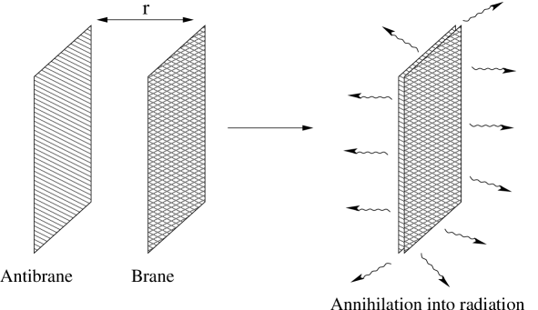
Figure 5.1: Brane-antibrane inflation and reheating.

There are two (or more) branes separated by a distance $r$. This distance $r$ plays the role of the inflaton in the 4D effective theory. When the distance between the branes is of order $1/M_{s}$, where $M_{s}$ is the string mass scale, the field becomes tachyonic and inflation ends. From a 4D viewpoint brane-antibrane inflation is very similar to hybrid inflation.

For a large separation, the interaction energy between the $D3/\overline{D3}$ pair is [95]

$$V(r)=2T_{3}\left(1-\frac{1}{2\pi^{3}}\frac{T_{3}}{M_{(10)}^{8}r^{4}}\right),$$ (5.4)

where $T_{3}$ is the tension of the $D3$-brane, $M_{(10)}^{2}$ is the 10D Planck mass and it is given by

$$M_{(10)}^{8}=\frac{M_{Pl}^{2}}{L^{6}},$$ (5.5)

where $M_{Pl}^{2}$ is the 4D Planck mass and $L^{6}$ is the volume of the compact manifold.

There is a problem with this model/potential. If one defines the usual slow-roll parameters as

$$\varepsilon=\frac{M_{Pl}^{2}}{2}\left(\frac{V^{\prime}}{V}\right)^{2},\quad\eta=M_{Pl}^{2}\frac{V^{\prime\prime}}{V},$$ (5.6)

where a prime denotes derivative with respect to the canonically normalized field $\phi$, given by $\phi=\sqrt{T_{3}}r$, then to have long lasting inflation we need $\varepsilon,\eta\ll 1$. For the potential (5.4)

$$\eta\sim-0.3\left(\frac{L}{r}\right)^{6},$$ (5.7)

and $\eta\ll 1$ is only possible if $r>L$. To have $r>L$ is impossible in a manifold of size $L$. One possible and natural way to evade this $\eta$-problem is to consider brane inflation in a warped geometry [95]. We will discuss such models in the next section.

5.3 The KKLMMT model: slow-moving brane

In this section, we present the Kachru et al. (KKLMMT) model [95] of warped brane inflation. They consider a $D3$-brane and an anti-$D3$-brane in a 5D anti-de-Sitter space ($AdS_{5}$). In [95], the authors also provide a concrete example of warped brane inflation in string theory. In that case the $AdS_{5}$ is replaced by the Klebanov-Strassler geometry [39], but the latter can be well approximated by $AdS_{5}\times S^{5}$ in the region far away from the tip of the geometry and this is a region of interest to study inflation. Thus, we shall present the $AdS_{5}$ case because it captures the essential features despite being simpler.

The $\overline{D3}$-brane is fixed at the infrared end of the geometry (region with small values of the warp factor). The $D3$-brane is mobile and experiences a small attractive force towards the $\overline{D3}$-brane as in figure 5.2. If the $\overline{D3}$-brane(s) were to be absent then the $D3$-brane would feel no force in this background as the electrostatic repulsion coming from the 5-form background flux exactly cancels the gravitational attraction.

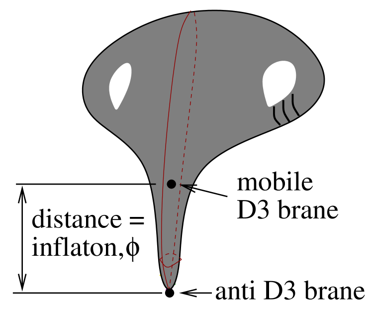
Figure 5.2: $D3$ and $\overline{D3}$ branes in the KKLMMT model. From [1].

They consider a string theory compactification on $AdS_{5}\times S^{5}$. It is a solution of the 10D supergravity with a 5-form field strength $F_{5}$. The metric is

$$ds^{2}=h^{-\frac{1}{2}}\eta_{\mu\nu}dx^{\mu}dx^{\nu}+h^{\frac{1}{2}}dr^{2},$$ (5.8)

where the warp factor $h$ is $h=R^{4}/r^{4}$. $R$ is the characteristic length scale of the $AdS_{5}$ spacetime and it is related to the 5-form charge. We choose to truncate the $AdS_{5}$ to the region where $r_{0}<r<r_{max}$. From (5.8) one sees that the region of small $r$ is the bottom of the gravitational well, this justifies the assumption of placing the $\overline{D3}$-brane(s) at the infrared end of the geometry. We denote the position of the $\overline{D3}$-brane by $r_{0}$. The background 5-form field is

$$\left(F_{5}\right)_{rx^{\mu}}=\frac{4r^{3}}{R^{4}},$$ (5.9)

and the 4-form gauge potential $C_{4}$ is

$$\left(C_{4}\right)_{x^{\mu}}=\frac{r^{4}}{R^{4}}.$$ (5.10)

The location of the $D3$-brane is denoted by $r_{1}$. The motion of the $D3$-brane is described by the Born-Infeld action plus the Chern-Simons action as

$$S=-T_{3}\int d^{4}x\sqrt{-g}\frac{r_{1}^{4}}{R^{4}}\sqrt{1-\frac{R^{4}}{r_{1}^{4}}g^{\mu\nu}\partial_{\mu}r_{1}\partial_{\nu}r_{1}}+T_{3}\int d^{4}x\left(C_{4}\right)_{x^{\mu}},$$ (5.11)

where $g^{\mu\nu}$ is the inverse metric along the non-compact directions. $T_{3}$ is the $D3$-brane tension. The action for a $\overline{D3}$-brane is similar to the previous action with the sign of the second term changed, because a $\overline{D3}$-brane has opposite 5-form charge. Now it is easy to see that if the $D3$-brane is slow-moving and there are no $\overline{D3}$-branes then the two contributions in (5.11) cancel each other partially to give

$$S=T_{3}\int d^{4}x\sqrt{-g}\frac{1}{2}g^{\mu\nu}\partial_{\mu}r_{1}\partial_{\mu}r_{1}.$$ (5.12)

This means that at low energies the $D3$-brane behaves as a free field.

Now, if we introduce a single $\overline{D3}$-brane this will perturb the metric and the $F_{5}$. The $D3$-brane will acquire a potential energy as [95]

$$V=2T_{3}\frac{r_{0}^{4}}{R^{4}}\left(1-\frac{1}{N}\frac{r_{0}^{4}}{r_{1}^{4}}\right),$$ (5.13)

where $N$ is the number of $D3$-branes that are present elsewhere in the manifold and create the warping. The previous expression is valid in the limit $r_{1}\gg r_{0}$. The first term is a constant potential energy due to the presence of the $\overline{D3}$-brane, but the effective tension of the antibrane is reduced by a factor $r_{0}^{4}/R^{4}$. The second term is location dependent and the minus sign indicates attraction between the branes. It is slow varying as the inverse fourth power of the radial location of the $D3$-brane. This term is also suppressed relatively to the first constant term. Then we can naturally get $\varepsilon,\eta\ll 1$.

This model is not totally free of problems, in particular a version of the so-called $\eta$-problem discussed in the previous section is still present due to coupling to gravity, see [95] for details.

5.4 The DBI model: “relativistic” regime

We have seen in the previous section that if the brane is moving slowly (“slow-roll” regime) and if the potential is flat enough then inflation occurs. References [110, 111, 112, 113] noted that inflation is also possible in a different regime of the parameter space. They realized that inflation is possible even if the potential is steep and the $D3$-brane is “relativistic”. In their model, the warped geometry slows down the inflaton field even on a steep potential. They called this model DBI-inflation because the action that governs the movement of the brane has the form of the DBI action. It reads

$$S\!\!\! = \!\!\!\frac{M^{2}_{Pl}}{2}\int d^{4}x\sqrt{-g}R$$ (5.14)

$$\!\!\!\!\!\!-\int d^{4}x\sqrt{-g}\left(f(\phi)^{-1}\sqrt{1+f(\phi)g^{\mu\nu}\partial_{\mu}\phi\partial_{\nu}\phi}-f(\phi)^{-1}+V(\phi)\right),$$

where $f(\phi)$ is related to the warp factor and $\phi$ is the rescaled position of the $D3$-brane in the throat. $V(\phi)$ is the potential energy that arises from interactions with the background fields. For an $AdS$-like throat, $f(\phi)\propto\phi^{-4}$.

There are two different situations that have been studied in the literature. The ultraviolet (UV) model [110, 111], where the inflaton moves from the UV side of the throat to the tip of the geometry (the infrared (IR) side), under the potential

$$V(\phi)\simeq\frac{1}{2}m^{2}\phi^{2},\quad m\gg\frac{M_{Pl}}{\sqrt{\lambda}},$$ (5.15)

where $\lambda$ is a parameter that depends on the background fluxes.

The other model that has been studied is the IR model [112, 113], where the brane moves away from the tip of the throat towards the Calabi-Yau part of the manifold. In this case the potential is

$$V(\phi)\simeq V_{0}-\frac{1}{2}m^{2}\phi^{2},\quad m\sim H.$$ (5.16)

In the spatially homogeneous case the Lagrangian is

$$P(X,\phi)=-f(\phi)^{-1}\sqrt{1-2Xf(\phi)}+f(\phi)^{-1}-V(\phi),$$ (5.17)

where $X$ is defined as $X=-1/2\partial^{\mu}\phi\partial_{\mu}\phi=\dot{\phi}^{2}/2$. The requirement that the argument of the square root in the Lagrangian has to be non-negative gives a speed limit for the inflaton as

$$1-f\dot{\phi}^{2}\geq 0.$$ (5.18)

We can define the speed of sound $c_{s}$ as $c_{s}=\sqrt{1-f\dot{\phi}^{2}}$. If the inflaton’s speed is close to saturating the previous bound its speed is said to be relativistic. In this case, $c_{s}\ll 1$ and $\dot{\phi}\simeq\pm 1/\sqrt{f(\phi)}$. The requirement that $\epsilon\equiv-\frac{\dot{H}}{H^{2}}\ll 1$ implies that the potential energy dominates over the kinetic energy during inflation despite the fact that the inflaton is moving relativistically.

In the next chapter, we shall study linear and non-linear perturbations of general models of inflation that include DBI-inflation as a particular case. We will be interested in calculating the higher-order statistics of the curvature perturbation.

5.5 Multiple field DBI-inflation

So far in this introductory chapter we have only discussed single field models of brane inflation. The inflaton field was identified with the position of a $D3$-brane in a higher-dimensional spacetime, like an $AdS_{5}$ throat for example. However, in more realistic string theory compactifications [13, 95] the throat is a 6D space that possesses a radial direction but also five angular coordinates. In general, one expects a probe $D3$-brane to move in all these directions. From a 4D effective theory point of view, each of these positions of the brane in the compact space is described by a 4D scalar field. Thus, DBI-inflation is naturally a multiple field inflationary model.

Some cosmological implications of including angular momentum in DBI brane inflation have been considered in [114, 115]. Due to some confusion in recent literature about the correct action for multi-field DBI-inflation here we shall outline the derivation of the multi-field DBI action [116, 117].

We consider a $D3$-brane with tension $T_{3}$ moving in a 10D warped string compactification. The 10D metric is

$$ds^{2}=H_{AB}dY^{A}dY^{B}=h^{-\frac{1}{2}}(y^{K})g_{\mu\nu}dx^{\mu}dx^{\nu}+h^{\frac{1}{2}}(y^{K})G_{IJ}(y^{K})dy^{I}dy^{J},$$ (5.19)

where $h$ is the warp factor, $g_{\mu\nu}$ and $x^{\mu}$ denote the metric and the coordinates of the 4D non-compact space respectively. $G_{IJ}$ and $y^{I}$ are the metric and the coordinates of the 6D internal space respectively. The 10D coordinates are denoted by $Y^{A}=\{x^{\mu},y^{I}\}$. The dynamics of the $D3$-brane is described by the DBI Lagrangian

$$P=-T_{3}\sqrt{-\mathrm{det}\gamma_{\mu\nu}},$$ (5.20)

where $\mathrm{det}$ denotes the determinant and $\gamma_{\mu\nu}$ is the induced metric on the brane. The induced metric is given by

$$\gamma_{\mu\nu}=H_{AB}\partial_{\mu}Y^{A}_{(b)}\partial_{\nu}Y^{B}_{(b)},$$ (5.21)

where $Y^{A}_{(b)}(x^{\mu})$ is the brane embedding. They are given by $Y^{A}_{(b)}=\left(x^{\mu},\varphi^{I}(x^{\mu})\right)$. Finally the induced metric on the brane can be written as

$$\gamma_{\mu\nu}=h^{-\frac{1}{2}}\left(g_{\mu\nu}+hG_{IJ}\partial_{\mu}\varphi^{I}\partial_{\nu}\varphi^{J}\right).$$ (5.22)

This implies that the DBI Lagrangian is

$$P=-T_{3}h^{-1}\sqrt{-g}\sqrt{\mathrm{det}\left(\delta_{\nu}^{\mu}+hG_{IJ}\partial^{\mu}\varphi^{I}\partial_{\nu}\varphi^{J}\right)}.$$ (5.23)

Introducing the rescaled quantities

$$f=\frac{h}{T_{3}},\quad\phi^{I}=\sqrt{T_{3}}\varphi^{I},$$ (5.24)

and a potential $V\left(\phi^{I}\right)$, the DBI Lagrangian is

$$P=-f(\phi^{I})^{-1}\left(\sqrt{\mathcal{D}}-1\right)-V(\phi^{I}),$$ (5.25)

where

$$\mathcal{D}=\mathrm{det}\left(\delta_{\nu}^{\mu}+fG_{IJ}\partial^{\mu}\phi^{I}\partial_{\nu}\phi^{J}\right).$$ (5.26)

The potential results from the interaction of the brane with background fields and has been explicitly calculated in some particular cases. For the rest of this work the potential is left unspecified and general.

It is useful to define a “kinetic matrix” as

$$X^{IJ}=-\frac{1}{2}\partial_{\mu}\phi^{I}\partial^{\mu}\phi^{J}.$$ (5.27)

Noting that

$$\mathrm{det}(A)=-\frac{1}{4!}\varepsilon_{\alpha_{1}\alpha_{2}\alpha_{3}\alpha_{4}}\varepsilon^{\beta_{1}\beta_{2}\beta_{3}\beta_{4}}A_{\beta_{1}}^{\alpha_{1}}A_{\beta_{2}}^{\alpha_{2}}A_{\beta_{3}}^{\alpha_{3}}A_{\beta_{4}}^{\alpha_{4}},$$ (5.28)

where

$$A_{\beta}^{\alpha}=\delta_{\beta}^{\alpha}+fB_{I}^{\alpha}B_{\beta}^{I},\quad B_{I}^{\alpha}\equiv G_{IJ}\partial^{\alpha}\phi^{J},\quad B_{\beta}^{I}\equiv\partial_{\beta}\phi^{I},$$ (5.29)

and after using the identity

$$\varepsilon_{\alpha_{1}\alpha_{2}\alpha_{3}\alpha_{4}}\varepsilon^{\alpha_{1}\cdots\alpha_{j}\beta_{j+1}\cdots\beta_{4}}=-(4-j)!j!\delta_{\alpha_{j+1}}^{[\beta_{j+1}}\cdots\delta_{\alpha_{4}}^{\beta_{4}]},$$ (5.30)

one can show that

$$\mathcal{D}=1-2fG_{IJ}X^{IJ}+4f^{2}X_{I}^{[I}X_{J}^{J]}-8f^{3}X_{I}^{[I}X_{J}^{J}X_{K}^{K]}+16f^{4}X_{I}^{[I}X_{J}^{J}X_{K}^{K}X_{L}^{L]}.$$ (5.31)

Because of the antisymmetrization over the field indices the last term vanishes if there are at most three fields. For two fields the last two terms of the previous expression vanish. For the single field case only the first two terms remain and one recovers the result obtained in single field DBI-inflation presented in the previous section. It turns out that the non-linear terms in $X^{IJ}$ of equation (5.31) also vanish for a multi-field DBI model if one considers homogeneous configurations, i.e., configurations in which the fields only depend on time and $X^{IJ}$ is given by $X^{IJ}=1/2\dot{\phi}^{I}\dot{\phi}^{J}$. This fact mislead the authors of [114, 115, 118] to ignore these terms even in the inhomogeneous case. References [116, 117] pointed out the importance of these terms and correctly conclude that they cannot be ignored. Because of these terms multi-field DBI-inflation is not a particular case of multi-field K-inflation as previously thought. In chapter 7, we will study linear and non-linear perturbations in general multiple field inflationary model. This general class of models includes K-inflation and DBI-inflation as particular examples. We shall also discuss the non-Gaussianity produced in these models, focusing in the three point functions of the adiabatic and entropy perturbations.

Chapter 6 Non-Gaussianity from the trispectrum in general single field inflation

6.1 Introduction

The theory of slow-roll inflation generically predicts that the observed cosmic microwave background radiation (CMBR) anisotropies are nearly scale invariant and very Gaussian. Indeed, the latest observations of CMBR by WMAP5 [107] confirm these expectations. This constitutes one of the biggest achievements of modern cosmology.

Despite its successes the theory of inflation still has many open questions. For example, we do not know the origin of the scalar field whose energy drives inflation, not to mention that we have never detected directly in the laboratory these kind of particles. The energy scale at which inflation happened is unknown by many orders of magnitude. There are many models of inflation that give similar predictions for the power spectrum of primordial perturbations, so which one (if any) is the correct one?

For us to move a step forward in our understanding of the very early universe we have to work on two fronts. First the observational side. In the next few years, with improved experiments like the Planck satellite, we will measure the CMBR anisotropies to an incredible resolution. For example the observational bounds on the bispectrum (the three point correlation function of the primordial curvature perturbation $\zeta$) will shrink from the present WMAP5 value $-9<f_{NL}<111$ [107] to $|f_{NL}|\lesssim 5$ [119], where the parameter $f_{NL}$ parameterizes the size of the bispectrum. It is because this parameter is constrained to be small that we say that the CMBR anisotropies are very Gaussian. The observational bounds on the trispectrum (four point function) will also tighten significantly from the rather weak present constraint of $|\tau_{NL}|<10^{8}$ [120, 121] to the future constraint of $|\tau_{NL}|\sim 560$ [122], where $\tau_{NL}$ denotes the size of the trispectrum. These previous observational bounds on the non-linearity parameters are for non-Gaussianity of the local type. These bounds change depending on the shape of the wave vectors’ configuration [123]. This is one of the reasons why it is important to calculate the shape dependence of the non-Gaussianity.

In face of these expected observational advances, it is then imperative to push forward our theoretical knowledge of our theories and calculate more observational consequences of the different inflationary models to make a comparison with observations possible. One possible direction to be followed by us and many others is to calculate higher order statistics (like the trispectrum) of the primordial curvature perturbation. These higher order statistics contain much more information about the inflationary dynamics and if we observe them they will strongly constrain our models. Because these higher order statistics have a non-trivial momentum dependence (shape) they will help to discriminate between models that have a similar power spectrum (two point function).

Calculations of the bispectrum for a single field inflationary model were done by Maldacena [124]. He showed that the primordial bispectrum is too small (of the order of the slow-roll parameters) to be observed even with Planck. Subsequent work generalized Maldacena’s result to include more fields and more complicated kinetic terms [125, 126, 127]. In [127], Chen et al. have calculated the bispectrum for a quite general model of single field inflation. They showed that for some models even the next-to-leading order corrections in the slow-roll expansion may be observed.

In this chapter, we will focus our attention on the calculation of the trispectrum. In [128], Seery et al. have calculated the trispectrum for slow-roll multi-field models (with standard kinetic terms) and they showed that at horizon crossing it is too small to be observed. But there are models of single field inflation, well motivated from more fundamental theories, that can produce a significant amount of non-Gaussianity, such as Dirac-Born-Infeld (DBI) inflation [111, 129]. In [129] the authors have computed the trispectrum for a model where the inflaton’s Lagrangian is a general function of the field’s kinetic energy and the field’s value, their result was obtained using a simple method [130], that only gives the correct leading order answer. In this chapter we will provide the equations necessary to calculate the next-to-leading order corrections to the trispectrum. We argue that for some models these corrections might become equally observable in the future. In fact, we will calculate the fourth order action in the uniform curvature gauge that is exact in the slow-roll expansion and therefore in principle one could calculate all slow-roll corrections to the trispectrum of the field perturbations.

We will also compute the exact fourth order action for the curvature perturbation $\zeta$ in the comoving gauge. For a simpler inflation model (with the standard kinetic term) this was recently done in [131]. However [131] did not consider second order tensor perturbations. We will argue that this is an oversimplification that leads to erroneous results. The reason simply being that at second order in perturbation theory, scalar degrees of freedom will source second order tensor perturbations and this will give a non-zero contribution for the fourth order action and hence the trispectrum.

There are other reasons why we will perform the calculation in the comoving gauge. First of all, in doing so we work all the time with the gauge invariant variable $\zeta$ that is directly related with the observational quantities. The comoving gauge action can also be used for other practical purposes. For example, it can be used to calculate loop effects that can possibly have important observational consequences. It can also be used to calculate the trispectrum of models where the potential has a “feature” (see [132, 133] for an example of such calculation for the bispectrum). In the vicinity of the sudden potential “jump” the slow-roll approximation temporarily fails and one might get an enhancement of the trispectrum. There are well motivated models of brane inflation where the throat’s warp factor suddenly jumps [134].

This chapter is organized as follows. In the next section, we introduce the model under consideration. In section 6.3 we shall study non-linear perturbations. First, we compute the fourth order action in the comoving gauge including both scalar and second order tensor degrees of freedom. After that we compute the fourth order action in the uniform curvature gauge. In section 6.4, we present the formalism needed to calculate the trispectrum. In section 6.5, we calculate the leading order trispectrum using the comoving gauge action. We comment on previous works and on the observability of next-to-leading order corrections. Section 6.6 is devoted to conclusions.

6.2 The model

In this work, we will consider a fairly general class of models described by the following action

$$S=\frac{1}{2}\int d^{4}x\sqrt{-g}\left[M^{2}_{Pl}R+2P(X,\phi)\right],$$ (6.1)

where $\phi$ is the inflaton field, $M_{Pl}$ is the Planck mass that we will set to unity hereafter, $R$ is the Ricci scalar and $X\equiv-\frac{1}{2}g^{\mu\nu}\partial_{\mu}\phi\partial_{\nu}\phi$ is the inflaton’s kinetic energy. $g_{\mu\nu}$ is the metric tensor. We label the inflaton’s Lagrangian by $P$ and we assume that it is a well behaved function of two variables, the inflaton field and its kinetic energy.

This general field Lagrangian includes as particular cases the common slow-roll inflation model, DBI-inflation [110, 111] and K-inflation [135].

We are interested in flat, homogeneous and isotropic Friedman-Robertson-Walker universes described by the line element

$$ds^{2}=-dt^{2}+a^{2}(t)\delta_{ij}dx^{i}dx^{j},$$ (6.2)

where $a(t)$ is the scale factor. The Friedman equation and the continuity equation read

$$3H^{2}=\rho,$$ (6.3)

$$\dot{\rho}=-3H\left(\rho+P\right),$$ (6.4)

where the Hubble rate is $H=\dot{a}/a$, $\rho$ is the energy of the inflaton and it is given by

$$\rho=2XP_{,X}-P,$$ (6.5)

where $P_{,X}$ denotes the derivative of $P$ with respect to $X$.

It was shown in [136] that for this model the speed of propagation of scalar perturbations (“speed of sound”) is $c_{s}$ given by

$$c_{s}^{2}=\frac{P_{,X}}{\rho_{,X}}=\frac{P_{,X}}{P_{,X}+2XP_{,XX}}.$$ (6.6)

We define the slow variation parameters, analogues of the slow-roll parameters, as:

$$\epsilon=-\frac{\dot{H}}{H^{2}}=\frac{XP_{,X}}{H^{2}},$$ (6.7)

$$\eta=\frac{\dot{\epsilon}}{\epsilon H},$$ (6.8)

$$s=\frac{\dot{c_{s}}}{c_{s}H}.$$ (6.9)

We should note that these slow variation parameters are more general than the usual slow-roll parameters and that the smallness of these parameters does not imply that the field is rolling slowly. We assume that the rate of change of the speed of sound is small (as described by $s$) but $c_{s}$ is otherwise free to change between zero and one.

It is convenient to introduce the following parameters that describe the non-linear dependence of the Lagrangian on the kinetic energy:

$$\Sigma=XP_{,X}+2X^{2}P_{,XX}=\frac{H^{2}\epsilon}{c_{s}^{2}},$$ (6.10)

$$\lambda=X^{2}P_{,XX}+\frac{2}{3}X^{3}P_{,XXX},$$ (6.11)

$$\Pi=X^{3}P_{,XXX}+\frac{2}{5}X^{4}P_{,XXXX}.$$ (6.12)

These parameters are related to the size of the bispectrum and trispectrum. The power spectrum of the primordial quantum fluctuation was first derived in [136] and reads

$$P_{k}^{\zeta}=\frac{1}{36\pi^{2}}\frac{\rho^{2}}{\rho+P}=\frac{1}{8\pi^{2}}\frac{H^{2}}{c_{s}\epsilon},$$ (6.13)

where it should be evaluated at the time of horizon crossing ${c_{s}}_{*}k=a_{*}H_{*}$. The spectral index is

$$n_{s}-1=\frac{d\ln P_{k}^{\zeta}}{d\ln k}=-2\epsilon-\eta-s.$$ (6.14)

WMAP observations of the perturbations in the CMBR tell us that the previous power spectrum is almost scale invariant therefore implying that the three slow variation parameters should be small at horizon crossing, roughly of order $10^{-2}$.

6.3 Non-linear perturbations

In this section, we will consider perturbations of the background (6.2) beyond linear order. There is a vast literature on second order perturbations that is important when one is interested in calculating three point correlation functions, see for example [124, 125, 127, 137]. We are interested in non-Gaussianities that come from the trispectrum and so we need to use third order perturbation theory. For that we need to compute the fourth order in the perturbation action. In this section we will obtain the fourth order action in two different gauges. As a check on our calculations we will compute the leading order (in slow roll) trispectrum in both gauges. We will follow the pioneering approach developed by Maldacena [124] and used in several subsequent papers [125, 126, 129, 128].

For reasons that will become clear later it is convenient to use the ADM metric formalism [138]. The ADM line element reads

$$ds^{2}=-N^{2}dt^{2}+h_{ij}\left(dx^{i}+N^{i}dt\right)\left(dx^{j}+N^{j}dt\right),$$ (6.15)

where $N$ is the lapse function, $N^{i}$ is the shift vector and $h_{ij}$ is the 3D metric.

The action (6.1) becomes

$$S=\frac{1}{2}\int dtd^{3}x\sqrt{h}N\left({}^{(3)}\!R+2P\right)+\frac{1}{2}\int dtd^{3}x\sqrt{h}N^{-1}\left(E_{ij}E^{ij}-E^{2}\right).$$ (6.16)

The tensor $E_{ij}$ is defined as

$$E_{ij}=\frac{1}{2}\left(\dot{h}_{ij}-\nabla_{i}N_{j}-\nabla_{j}N_{i}\right),$$ (6.17)

and it is related to the extrinsic curvature by $K_{ij}=N^{-1}E_{ij}$. $\nabla_{i}$ is the covariant derivative with respect to $h_{ij}$ and all contra-variant indices in this section are raised with $h_{ij}$ unless stated otherwise.

The Hamiltonian and momentum constraints are respectively

$${}^{(3)}\!R+2P-2\pi^{2}N^{-2}P_{,X}-N^{-2}\left(E_{ij}E^{ij}-E^{2}\right) = 0,$$

$$\nabla_{j}\left(N^{-1}E_{i}^{j}\right)-\nabla_{i}\left(N^{-1}E\right) = \pi N^{-1}\nabla_{i}\phi P_{,X},$$ (6.18)

where $\pi$ is defined as

$$\pi\equiv\dot{\phi}-N^{j}\nabla_{j}\phi.$$ (6.19)

We decompose the shift vector $N^{i}$ into scalar and intrinsic vector parts as

$$N_{i}=\tilde{N_{i}}+\partial_{i}\psi,$$ (6.20)

where $\partial_{i}\tilde{N^{i}}=0$, here indices are raised with $\delta_{ij}$.

Before we consider perturbations around our background let us count the number of degrees of freedom (dof) that we have. There are five scalar functions, the field $\phi$, $N$, $\psi$, $\mbox{det}h$ and $h_{ij}\sim\partial_{i}\partial_{j}H$, where $H$ is a scalar function and $\mbox{det}h$ denotes the determinant of the 3D metric. Also, there are two vector modes $\tilde{N}^{i}$ and $h_{ij}\sim\partial_{i}\chi_{j}$, where $\chi^{j}$ is an arbitrary vector. Both $\tilde{N}^{i}$ and $\chi^{j}$ satisfy a divergenceless condition and so carry four dof. Furthermore, we also have a transverse and traceless tensor mode $\gamma_{ij}$ that contains two additional dof. Because our theory is invariant under change of coordinates we can eliminate some of these dof. For instance, a spatial reparametrization like $x^{i}=\tilde{x}^{i}+\partial^{i}\tilde{\epsilon}(\tilde{x},\tilde{t})+\epsilon^{i}_{(t)}(\tilde{x},\tilde{t})$, where $\tilde{\epsilon}$ and $\epsilon^{i}_{(t)}$ are arbitrary and $\partial_{i}\epsilon^{i}_{(t)}=0$, can be chosen so that it removes one scalar dof and one vector mode. A time reparametrization would eliminate another scalar dof. Constraints in the action will eliminate further two scalar dof and a vector mode. In the end we are left with one scalar, zero vector and one tensor modes that correspond to three physical propagating dof.

In the next subsection we shall use two different gauges that correctly parameterize these dof. Because physical observables are gauge invariant we know that both gauges have to give the same result for the trispectrum for instance. It seems then unnecessary to perform the calculation twice in different gauges. In practice, we will see that both gauges have advantages and disadvantages and one is more suitable for some applications than the other. Furthermore, it provides a good consistency check on the calculation.

6.3.1 Non-linear perturbations in the comoving gauge

In this subsection, we will compute the fourth order action for the general model (6.1) in the comoving gauge. In this gauge the scalar degree of freedom is the so-called curvature perturbation $\zeta$ that is also gauge invariant. There are a few works on this subject using this gauge, see e.g. [131], where the authors have calculated the fourth order action for a standard kinetic term inflation but they neglected second order tensor perturbations. We will show that this is an oversimplification that may lead to an erroneous result for the four point correlation function.

In the comoving gauge, the inflaton fluctuations vanish and the 3D metric is perturbed as

$$\delta\phi=0,$$

$$h_{ij}=a^{2}e^{2\zeta}\hat{h}_{ij},\quad\hat{h}_{ij}=\delta_{ij}+\gamma_{ij}+\frac{1}{2}\gamma_{ik}\gamma_{j}^{k}+\cdots$$ (6.21)

where $\mbox{det}\hat{h}=1$, $\gamma_{ij}$ is a tensor perturbation that we assume to be a second order quantity, i. e. $\gamma_{ij}=\mathcal{O}(\zeta^{2})$. It obeys the traceless and transverse conditions $\gamma_{i}^{i}=\partial^{i}\gamma_{ij}=0$ (indices are raised with $\delta_{ij}$). $\zeta$ is the gauge invariant scalar perturbation. In (6.21), we have ignored the first order tensor perturbations ${}^{(1)}{\gamma_{ij}}_{GW}$. This is because any correlation function involving this tensor mode will be smaller than a correlation function involving only scalars, see results of [124]. In the literature the second order tensor perturbations are often neglected, however they should be taken into account. The reason for this is because at second order the scalars will source the tensor perturbations equation. Later in this section, we will elaborate further on this point. Higher order tensor perturbations, like ${}^{(3)}\gamma_{ij}$, do not contribute to the fourth order action.

We expand $N$ and $N^{i}$ in power of the perturbation $\zeta$

$$N=1+\alpha_{1}+\alpha_{2}+\cdots,$$ (6.22)

$$\tilde{N_{i}}=\tilde{N_{i}}^{(1)}+\tilde{N_{i}}^{(2)}+\cdots,$$ (6.23)

$$\psi=\psi_{1}+\psi_{2}+\cdots,$$ (6.24)

where $\alpha_{n}$, $\tilde{N_{i}}^{(n)}$ and $\psi_{n}$ are of order $\zeta^{n}$.

Some useful expressions for the quantities appearing in (6.18), valid to all orders in perturbations but for $\gamma_{ij}=0$:

$${}^{(3)}\!R=-2a^{-2}e^{-2\zeta}\left(\partial_{i}\zeta\partial^{i}\zeta+2\partial_{i}\partial^{i}\zeta\right),$$ (6.25)

$$E_{ij}E^{ij}-E^{2} = -6\left(H+\dot{\zeta}\right)^{2}+\frac{4H}{a^{2}}\left(1+\frac{\dot{\zeta}}{H}\right)e^{-2\zeta}\left(\partial^{2}\psi+\partial^{k}\zeta\partial_{k}\psi+\partial^{k}\zeta\tilde{N}_{k}\right)$$ (6.26)

$$+a^{-4}e^{-4\zeta}\Bigg{[}\frac{1}{2}\partial_{i}\tilde{N}_{j}\left(\partial^{i}\tilde{N}^{j}+\partial^{j}\tilde{N}^{i}\right)+2\partial^{i}\partial^{j}\psi\partial_{i}\tilde{N}_{j}+\partial_{i}\partial_{j}\psi\partial^{i}\partial^{j}\psi$$

$$-\partial^{2}\psi\partial^{2}\psi-2\partial_{i}\tilde{N}_{j}\left(\partial^{j}\zeta\tilde{N}^{i}+\partial^{i}\zeta\tilde{N}^{j}\right)-4\tilde{N}_{k}\partial_{i}\zeta\partial^{i}\partial^{k}\psi$$

$$-2\partial_{i}\tilde{N}_{j}\left(\partial^{j}\zeta\partial^{i}\psi+\partial^{i}\zeta\partial^{j}\psi\right)-4\partial_{i}\partial_{j}\psi\partial^{j}\zeta\partial^{i}\psi$$

$$+2\partial^{j}\zeta\left(\partial_{j}\zeta\tilde{N}_{i}\tilde{N}^{i}+2\partial_{j}\zeta\tilde{N}_{i}\partial^{i}\psi+\partial_{j}\zeta\partial_{i}\psi\partial^{i}\psi\right)\Bigg{]},$$

$$\nabla_{j}\left(N^{-1}E_{i}^{j}\right)-\nabla_{i}\left(N^{-1}E\right)=$$

$$-N^{-2}\Bigg{[}-2\left(H+\dot{\zeta}\right)\partial_{i}N+\frac{a^{-2}e^{-2\zeta}}{2}\bigg{(}-\partial^{j}N\left(\partial_{i}N_{j}+\partial_{j}N_{i}\right)$$

$$\quad\quad\quad\quad+2\partial_{j}N\left(\partial^{j}\zeta N_{i}+\partial_{i}\zeta N^{j}\right)+2\partial_{i}N\partial^{2}\psi\bigg{)}\Bigg{]}$$

$$+N^{-1}\Bigg{[}-2\partial_{i}\dot{\zeta}+a^{-2}e^{-2\zeta}\bigg{(}\frac{1}{2}\left(\partial^{j}\zeta\partial_{j}\tilde{N}_{i}-\partial_{j}\zeta\partial_{i}\tilde{N}^{j}\right)+\partial_{j}\zeta\partial^{j}\zeta N_{i}-\partial_{i}\zeta\partial^{j}\zeta N_{j}$$

$$\quad\quad\quad\quad+\partial_{i}\partial^{j}\zeta N_{j}+\partial^{2}\zeta N_{i}-\frac{1}{2}\partial^{2}\tilde{N}_{i}\bigg{)}\Bigg{]}.$$ (6.27)

In the previous equations, indices in the right-hand side are raised with $\delta_{ij}$ while indices in the left-hand side are raised with $h_{ij}$. In the rest of this section indices will be raised with $\delta_{ij}$.

Now, the strategy is to solve the constraint equations for the lapse function and shift vector in terms of $\zeta$ and then plug in the solutions in the expanded action up to fourth order.

At first order in $\zeta$, a particular solution for equations (6.18) is [124, 125]:

$$\alpha_{1}=\frac{\dot{\zeta}}{H},\quad\tilde{N_{i}}^{(1)}=0,\quad\psi_{1}=-\frac{\zeta}{H}+\chi,\quad\partial^{2}\chi=a^{2}\frac{\epsilon}{c_{s}^{2}}\dot{\zeta}.$$ (6.28)

At second order, the constraint equation for the lapse function gives

$$\frac{4H}{a^{2}}\partial^{2}\psi_{2} = -2a^{-2}\partial_{i}\zeta\left(\partial^{i}\zeta+2H\partial^{i}\psi_{1}\right)-4\alpha_{1}\left(a^{-2}\partial_{i}\partial^{i}\zeta-2\Sigma\zeta\right)-2\alpha_{1}^{2}\left(\Sigma+6\lambda\right)$$ (6.29)

$$-a^{-4}\left(\partial^{i}\partial_{k}\psi_{1}\partial_{i}\partial^{k}\psi_{1}-\partial^{2}\psi_{1}\partial^{2}\psi_{1}\right)+4\alpha_{2}\left(\Sigma-3H^{2}\right),$$

and the equation for the shift vector gives

$$2H\partial_{i}\alpha_{2}-\frac{1}{2}a^{-2}\partial^{2}\tilde{N_{i}}^{\!\!(2)}=-a^{-2}\left(\partial_{k}\alpha_{1}\partial^{k}\partial_{i}\psi_{1}-\partial_{i}\alpha_{1}\partial^{2}\psi_{1}+\partial^{2}\zeta\partial_{i}\psi_{1}+\partial_{i}\partial^{k}\zeta\partial_{k}\psi_{1}\right).$$ (6.30)

Due to the fact that $\tilde{N^{i}}$ is divergenceless and that any vector can be separated into a incompressible and irrotational part one can separate the contributions from $\alpha_{2}$ and $\tilde{N_{i}}^{\!\!(2)}$ in the previous equation. The irrotational part of Eq. (6.30) gives

$$2H\alpha_{2}=\partial^{-2}\partial^{i}F_{i},$$ (6.31)

and the incompressible part gives

$$\frac{1}{2a^{2}}\tilde{N_{i}}^{\!\!(2)}=-\partial^{-2}F_{i}+\partial^{-4}\partial_{i}\partial^{k}F_{k},$$ (6.32)

where $F_{i}$ is defined as the right-hand side of equation (6.30). The operator $\partial^{-2}$ is defined by $\partial^{-2}(\partial^{2}\varphi)=\varphi$ and in Fourier space it just brings in a factor of $-1/k^{2}$.

It was shown in [127] that to compute the effective action of order $\zeta^{n}$, within the ADM formalism, one only needs to use the solution for the Lagrange multipliers $N$ and $N^{i}$ up to order $\zeta^{n-2}$. Therefore in order to calculate the fourth order effective action the knowledge of the Lagrange multipliers up to second order is required. It is given in equations (6.28), (6.31) and (6.32).

The second order action is

$$S_{2}=\int dtd^{3}x\left[a^{3}\frac{\epsilon}{c_{s}^{2}}\dot{\zeta}^{2}-a\epsilon\left(\partial\zeta\right)^{2}\right].$$ (6.33)

The third order action is [124, 125, 127]

$$S_{3}\!\! = \!\!\int dtd^{3}x\left[-\epsilon a\zeta\left(\partial\zeta\right)^{2}-a^{3}\left(\Sigma+2\lambda\right)\frac{\dot{\zeta}^{3}}{H^{3}}+\frac{3a^{3}\epsilon}{c_{s}^{2}}\zeta\dot{\zeta}^{2}\right.$$ (6.34)

$$\!\!\!\!\left.+\frac{1}{2a}\left(3\zeta-\frac{\dot{\zeta}}{H}\right)\left(\partial_{i}\partial_{j}\psi_{1}\partial_{i}\partial_{j}\psi_{1}-\partial^{2}\psi_{1}\partial^{2}\psi_{1}\right)-\frac{2}{a}\partial_{i}\psi_{1}\partial_{i}\zeta\partial^{2}\psi_{1}\right].$$

The scalar fourth order action is

$$S_{4}\!\! = \!\!\frac{1}{2}\int dtd^{3}xa^{3}\left[-a^{-2}\epsilon\zeta^{2}\left(\partial\zeta\right)^{2}+\alpha_{1}^{4}\left(2\Sigma+9\lambda+\frac{10}{3}\Pi\right)-6\zeta\alpha_{1}^{3}\left(\Sigma+2\lambda\right)\right.$$ (6.35)

$$\!\!\!\!-2\alpha_{2}^{2}\left(\Sigma-3H^{2}\right)+a^{-4}\left(\frac{\zeta^{2}}{2}+\zeta\alpha_{1}+\alpha_{1}^{2}\right)\left(\partial^{k}N_{j}^{(1)}\partial_{k}{N^{j}}^{(1)}-\partial^{j}N_{j}^{(1)}\partial^{k}N_{k}^{(1)}\right)$$

$$\!\!\!\!-2a^{-4}\left(\zeta+\alpha_{1}\right)\partial^{k}{N^{j}}^{(1)}\left(\partial_{k}N_{j}^{(2)}-\delta_{kj}\partial^{n}N_{n}^{(2)}-2\partial_{j}\zeta N_{k}^{(1)}\right)$$

$$\!\!\!\!+a^{-4}\left(-4\partial_{k}N_{j}^{(1)}\partial^{j}\zeta{N^{k}}^{(2)}+2N_{k}^{(1)}\partial_{j}\zeta{N^{k}}^{(1)}\partial^{j}\zeta\right)+9\zeta^{2}\alpha_{1}^{2}\Sigma$$

$$\!\!\!\!\left.+\frac{a^{-4}}{2}\partial_{k}\tilde{N}_{j}^{(2)}\partial^{k}\tilde{N}^{j(2)}-2a^{-4}\partial_{k}N_{j}^{(2)}\left(\partial^{j}\zeta{N^{k}}^{(1)}+\partial^{k}\zeta{N^{j}}^{(1)}\right)\right].$$

Here, no slow-roll approximation has been made. The previous action has to be supplemented with the action containing terms with one and two tensors

$$S_{\gamma^{2}}=\frac{1}{8}\int dtd^{3}x\left[a^{3}\dot{\gamma}_{ij}\dot{\gamma}^{ij}-a\partial_{k}\gamma_{ij}\partial^{k}\gamma^{ij}\right],$$ (6.36)

$$S_{\gamma\zeta^{2}}=\int dtd^{3}x\Bigg{[} \!\!\!\!\!\!\!\!\!\!-2\frac{a}{H}\gamma_{ij}\partial^{i}\dot{\zeta}\partial^{j}\zeta-a\gamma_{ij}\partial^{i}\zeta\partial^{j}\zeta-\frac{1}{2}a\left(3\zeta-\frac{\dot{\zeta}}{H}\right)\dot{\gamma}_{ij}\partial^{i}\partial^{j}\psi_{1}$$ (6.37)

$$\!\!\!\!\!\!\!\!\!\!+\frac{1}{2}a^{-1}\partial_{k}\gamma_{ij}\partial^{i}\partial^{j}\psi_{1}\partial^{k}\psi_{1}\Bigg{]}.$$

Canonical variable for quantization $\zeta_{n}$

In order to calculate the quantum four point correlation function we follow the standard procedure in quantum field theory. However there is an important subtlety here. The gauge invariant quantity $\zeta$ is not the correct variable to be quantized, because it is not a canonical field . The canonical field to be quantized is the field perturbation $\delta\phi$, or a convenient parameterization $\zeta_{n}$ defined by

$$\zeta_{n}=-\frac{H}{\dot{\phi}_{0}}\delta\phi,$$ (6.38)

where $\phi_{0}$ is the background value of the field. We will see that $\zeta$ is related to $\zeta_{n}$ by a non-linear transformation so for the power spectrum calculation both procedures of quantizing $\zeta$ or $\zeta_{n}$ give the same answer because the difference between these two variables is a second order quantity. However, for the calculation of higher order correlation functions (like the bispectrum or trispectrum) $\zeta_{n}$ is the correct variable to be quantized as it is linear in $\delta\phi$. For the trispectrum, quantizing $\zeta$ gives different results from quantizing $\zeta_{n}$. We will find the relation between $\zeta$ and $\zeta_{n}$ through the gauge transformation equations from the uniform curvature gauge (discussed in detail in the next subsection) to the comoving gauge. In the uniform curvature gauge the ansatz is

$$\phi(x,t)=\phi_{0}+\delta\phi(x,t),$$

$$h_{ij}=a^{2}\hat{h}_{ij},\quad\hat{h}_{ij}=\delta_{ij}+\tilde{\gamma}_{ij}+\frac{1}{2}\tilde{\gamma}_{ik}\tilde{\gamma}_{j}^{k}+\cdots$$ (6.39)

where $\mbox{det}\hat{h}=1$ and $\tilde{\gamma}_{ij}$ is a tensor perturbation that we assume to be a second order quantity, i.e., $\tilde{\gamma}_{ij}=\mathcal{O}(\delta\phi^{2})$. The gauge transformations are

$$\zeta(\mathbf{x}) = \zeta_{n}(\mathbf{x})+F_{2}(\zeta_{n}(\mathbf{x}))+F_{3}(\zeta_{n}(\mathbf{x})),$$ (6.40)

$$\gamma_{ij} = \tilde{\gamma}_{ij}(t)+\mu_{ij},$$ (6.41)

where $F_{2}(\zeta_{n}),\mu_{ij}=\mathcal{O}(\zeta_{n}^{2})$, $F_{3}(\zeta_{n})=\mathcal{O}(\zeta_{n}^{3})$ are the terms coming from the second and third order gauge transformations respectively, they can be found explicitly in appendix C or in [124, 131].

We now need to find the fourth order action for the variable $\zeta_{n}$. Schematically, we write the different contributions as

$$S_{\zeta_{n}}=S_{4}(\zeta_{n})+S_{\gamma^{2}}(\zeta_{n})+S_{\gamma\zeta^{2}}(\zeta_{n})+S_{3}(F_{2}(\zeta_{n}))+S_{2}(F_{2}(\zeta_{n})).$$ (6.42)

The first three terms come from Eqs. (6.35-6.37) when we substitute $\zeta$ with $\zeta_{n}$ and $\gamma_{ij}$ with Eq. (6.41). Due to the non-linear relation between $\zeta$ and $\zeta_{n}$, the third order action for $\zeta$, Eq. (6.34), will after the change of variables give a contribution to the fourth order action like $S_{3}(F_{2}(\zeta_{n}))$. Similarly, the second order action, Eq. (6.33), will also contribute with $S_{2}(F_{2}(\zeta_{n}))$. In principle, one would also need to compute the third order gauge transformation as the second order action gives origin to fourth order terms like $\dot{\zeta_{n}}\dot{F}_{3}(\zeta_{n})$ (where $F_{3}(\zeta_{n})$ is the third order piece of the gauge transformation). Fortunately, terms involving $F_{3}$ can be shown to be proportional to the first order equations of motion for $\zeta_{n}$, therefore when computing the trispectrum these terms will vanish and we do not need to calculate the third order gauge transformation explicitly at this point. It can be easily seen that equations (6.34), (6.35), (6.36), (6.37) or their counterparts in terms of $\zeta_{n}$, Eq. (6.42), have terms that are not slow roll suppressed. However, because in pure de Sitter space $\zeta$ is a gauge mode we expect the action (6.42) to be slow-roll suppressed (of order $\epsilon$). One can perform many integrations by parts to show that the unsuppressed terms of (6.42) can be reduced to total derivative terms and slow-roll suppressed terms given by

$$S_{parts}=\int dt \!\!\!\!\!\!\!\!\!\!d^{3}x\Big{\{}-\frac{3\epsilon}{aH^{2}}\Big{[}\frac{1}{4}\left(\partial_{j}\zeta_{n}\partial^{j}\zeta_{n}\right)^{2}+\frac{1}{8}\zeta_{n}^{2}\partial^{2}\left(\partial_{j}\zeta_{n}\partial^{j}\zeta_{n}\right)$$ (6.43)

$$+\partial_{j}\zeta_{n}\partial^{j}\zeta_{n}\partial^{-2}\partial^{l}\partial^{k}\left(\partial_{l}\zeta_{n}\partial_{k}\zeta_{n}\right)+2\partial_{i}\left(\partial^{k}\zeta_{n}\partial^{i}\zeta_{n}\right)\partial^{-2}\partial_{l}\left(\partial_{k}\zeta_{n}\partial^{l}\zeta_{n}\right)$$

$$+\frac{1}{2}\left(\partial^{-2}\partial_{j}\partial_{k}\left(\partial^{j}\zeta_{n}\partial^{k}\zeta_{n}\right)\right)^{2}\Big{]}$$

$$-\frac{5\epsilon}{8a^{3}H^{4}}\Big{[}\partial_{l}\zeta_{n}\partial^{l}\zeta_{n}\partial^{k}\partial^{j}\left(\partial_{k}\zeta_{n}\partial_{j}\zeta_{n}\right)-\frac{1}{2}\partial_{j}\zeta_{n}\partial^{j}\zeta_{n}\partial^{2}\left(\partial_{k}\zeta_{n}\partial^{k}\zeta_{n}\right)$$

$$\;\;\;\;\;\;\;\;\;\;\;\;\;\;\;\;\;\;-\frac{1}{2}\partial^{k}\partial^{j}\left(\partial_{k}\zeta_{n}\partial_{j}\zeta_{n}\right)\partial^{-2}\partial^{m}\partial^{l}\left(\partial_{m}\zeta_{n}\partial_{l}\zeta_{n}\right)\Big{]}\Big{\}}.$$

For us to be able to obtain the previous result it is crucial to include the contributions from the tensor actions (6.36) and (6.37), otherwise the trispectrum calculated using the $\mathcal{O}(\epsilon^{0})$ of (6.35) does not vanish, giving the wrong leading order result. Neglecting tensor perturbations (sourced by the scalars) for the calculation of the trispectrum is not consistent and leads to wrong results. This is one of the results of our work. The contribution from $\tilde{\gamma}_{ij}$ that comes through $\gamma_{ij}$ in (6.36) and (6.37) will result in terms that are already slow-roll suppressed and no further integrations by parts are need on these terms (see Eq. (6.59) of next subsection). The final action for $\zeta_{n}$ is then

$${S_{4}}_{\zeta_{n}}=S_{\zeta_{n}}^{(\epsilon)}+S_{parts},$$ (6.44)

where $S_{\zeta_{n}}^{(\epsilon)}$ denotes the terms of (6.42) that are suppressed by at least one slow-roll parameter. This final action is slow-roll suppressed as expected and no slow-roll approximation was made so it is also exact.

6.3.2 Non-linear perturbations in the uniform curvature gauge

In order to calculate the intrinsic four point correlation function of the field perturbation we need to compute the action of fourth order in the perturbations. In this subsection we will obtain the fourth order action in the uniform curvature gauge. In this gauge, the scalar degree of freedom is the inflaton field perturbation $\delta\phi(x^{\mu})$. There are several works in the literature where the authors also calculate the trispectrum. In [128], Seery et al. calculate the trispectrum of a multi-field inflation model, however the result is only valid for fields with standard kinetic energies, i.e. $P(X_{1},\ldots,X_{n},\phi_{1},\ldots,\phi_{n})=X_{1}+\cdots+X_{n}-V$, where $X_{n}$ is the kinetic energy of $\phi_{n}$ and $V$ is the potential. In this chapter we will generalize their result for an arbitrary function $P(X,\phi)$ but for single field only. Recently, Huang and Shiu have obtained the fourth order action for the model under consideration (6.1). However the result was obtained by only perturbing the field Lagrangian. This procedure gives the right result as long as we are interested in the leading order contribution in the small speed of sound limit and in the slow-roll approximation, which was their case of interest. In the present section we will compute the fourth order action that is valid to all orders in slow roll and in the sound of speed expansion. To do that we have to perturb the full action (6.1) up to fourth order in the field perturbations. The procedure to obtain the fourth order action in this gauge is similar to the one used in subsection 6.3.1.

In this gauge, the inflaton perturbation does not vanish and the 3D metric takes the form

$$\phi(x,t)=\phi_{0}+\delta\phi(x,t),$$

$$h_{ij}=a^{2}\hat{h}_{ij},\quad\hat{h}_{ij}=\delta_{ij}+\tilde{\gamma}_{ij}+\frac{1}{2}\tilde{\gamma}_{ik}\tilde{\gamma}_{j}^{k}+\cdots$$ (6.45)

where $\mbox{det}\hat{h}=1$ and $\tilde{\gamma}_{ij}$ is a tensor perturbation that we assume to be a second order quantity, i.e., $\tilde{\gamma}_{ij}=\mathcal{O}(\delta\phi^{2})$. It obeys the traceless and transverse conditions $\tilde{\gamma}_{i}^{i}=\partial^{i}\tilde{\gamma}_{ij}=0$ (indices are raised with $\delta_{ij}$). In the literature the second order tensor perturbations are often neglected, however based on our results it should be taken into account. We can always use the gauge freedom at second order to eliminate the trace and the vector perturbations of $h_{ij}$. The presence of $\tilde{\gamma}_{ij}$ makes the three dimensional hypersurfaces non-flat so using the name uniform curvature gauge might be misleading.

We expand $N$ and $N^{i}$ in powers of the perturbation $\delta\phi(x,t)$

$$N=1+\alpha_{1}+\alpha_{2}+\cdots,$$ (6.46)

$$\tilde{N_{i}}=\tilde{N_{i}}^{(1)}+\tilde{N_{i}}^{(2)}+\cdots,$$ (6.47)

$$\psi=\psi_{1}+\psi_{2}+\cdots,$$ (6.48)

where $\alpha_{n}$, $\tilde{N_{i}}^{(n)}$ and $\psi_{n}$ are of order $\delta\phi^{n}$ and $\phi_{0}(t)$ is the background value of the field. At first order in $\delta\phi$, a particular solution for equations (6.18) is [124, 128]:

$$\alpha_{1}=\frac{1}{2H}\dot{\phi_{0}}\delta\phi P_{,X},\quad\tilde{N_{i}}^{(1)}=0,\quad\partial^{2}\psi_{1}=\frac{a^{2}\epsilon}{c_{s}^{2}}\frac{d}{dt}\left(-\frac{H}{\dot{\phi}}\delta\phi\right).$$ (6.49)

At second order, the constraint equation for the lapse function gives

$$\frac{4H}{a^{2}}\partial^{2}\psi_{2} = \frac{1}{a^{4}}\left(\partial^{2}\psi_{1}\partial^{2}\psi_{1}-\partial_{i}\partial_{j}\psi_{1}\partial^{i}\partial^{j}\psi_{1}\right)+6H^{2}\left(3\alpha_{1}^{2}-2\alpha_{2}\right)$$ (6.50)

$$+\frac{8H\alpha_{1}}{a^{2}}\partial^{2}\psi_{1}-\left(3\dot{\phi_{0}}^{2}\alpha_{1}^{2}-2\dot{\phi_{0}}^{2}\alpha_{2}+\dot{\delta\phi}^{2}-4\dot{\phi_{0}}\dot{\delta\phi}\alpha_{1}\right)P_{,X}$$

$$-\frac{1}{a^{2}}\left(\partial_{i}\delta\phi\partial^{i}\delta\phi-2\dot{\phi_{0}}\partial_{i}\delta\phi\partial^{i}\psi_{1}\right)P_{,X}$$

$$+\delta\phi^{2}P_{,\phi\phi}+2\dot{\phi_{0}}\delta\phi\left(\dot{\phi_{0}}\alpha_{1}-\dot{\delta\phi}\right)P_{,X\phi}$$

$$-\frac{\dot{\phi_{0}}^{2}}{a^{2}}\bigg{(}-10a^{2}\dot{\phi_{0}}\dot{\delta\phi}\alpha_{1}-2\dot{\phi_{0}}\partial_{i}\delta\phi\partial^{i}\psi_{1}+6a^{2}\dot{\phi_{0}}^{2}\alpha_{1}^{2}$$

$$-2\dot{\phi_{0}}^{2}a^{2}\alpha_{2}+4a^{2}\dot{\delta\phi}^{2}-\partial_{i}\delta\phi\partial^{i}\delta\phi\bigg{)}P_{,XX}$$

$$-\dot{\phi_{0}}^{4}\left(\dot{\phi_{0}}^{2}\alpha_{1}^{2}+\dot{\delta\phi}^{2}-2\dot{\phi_{0}}\dot{\delta\phi}\alpha_{1}\right)P_{,XXX}$$

$$+2\dot{\phi_{0}}^{3}\delta\phi\left(\dot{\phi_{0}}\alpha_{1}-\dot{\delta\phi}\right)P_{,XX\phi}-\dot{\phi_{0}}^{2}\delta\phi^{2}P_{,X\phi\phi},$$

and the equation for the shift vector gives

$$2H\partial_{i}\alpha_{2}-\frac{1}{2}a^{-2}\partial^{2}\tilde{N_{i}}^{\!\!(2)} = 4\alpha_{1}H\partial_{i}\alpha_{1}+a^{-2}\left(\partial_{i}\alpha_{1}\partial^{2}\psi_{1}-\partial_{k}\alpha_{1}\partial_{i}\partial^{k}\psi_{1}\right)$$ (6.51)

$$+\partial_{i}\delta\phi\left(\dot{\delta\phi}-\dot{\phi_{0}}\alpha_{1}\right)P_{,X}+\partial_{i}\delta\phi\dot{\phi_{0}}^{2}\left(\dot{\delta\phi}-\dot{\phi_{0}}\alpha_{1}\right)P_{,XX}$$

$$+\partial_{i}\delta\phi\dot{\phi_{0}}\delta\phi P_{,X\phi},$$

where $P_{,\phi}$ means derivative of $P$ with respect to $\phi$.

Due to the fact that $\tilde{N^{i}}$ is divergenceless and that any vector can be separated into a incompressible and irrotational part one can separate the contributions from $\alpha_{2}$ and $\tilde{N_{i}}^{\!\!(2)}$ in the previous equation. The irrotational part of Eq. (6.51) gives

$$2H\alpha_{2}=\partial^{-2}\partial^{i}F_{i},$$ (6.52)

and the incompressible part gives

$$\frac{1}{2a^{2}}\tilde{N_{i}}^{\!\!(2)}=-\partial^{-2}F_{i}+\partial^{-4}\partial_{i}\partial^{k}F_{k},$$ (6.53)

where $F_{i}$ is defined as the right-hand side of equation (6.51).

The scalar fourth order action, where no slow-roll approximation has been made, is

$$S_{4}=S_{A}+S_{B},$$ (6.54)

where

$$S_{A} \!\!= \!\!\int dtd^{3}x\Bigg{[}-\frac{a\delta\phi}{2}\Big{[}a^{2}\alpha_{1}\dot{\delta\phi}^{2}+2\partial_{i}\delta\phi\partial^{i}\psi_{1}\left(\dot{\delta\phi}-\alpha_{1}\dot{\phi}_{0}\right)+a^{2}\dot{\phi}_{0}^{2}\alpha_{1}^{3}+\alpha_{1}(\partial\delta\phi)^{2}$$ (6.55)

$$\!\!\!\!+2\dot{\phi}_{0}\partial^{i}\delta\phi\left(\tilde{N_{i}}^{\!\!(2)}+\partial_{i}\psi_{2}\right)\Big{]}P_{,X\phi}-\frac{1}{8a}\Big{[}4\dot{\phi}_{0}^{4}a^{4}\alpha_{2}\left(\alpha_{2}-2\alpha_{1}^{2}\right)+3\dot{\phi}_{0}^{4}a^{4}\alpha_{1}^{4}$$

$$\!\!\!\!-18\dot{\phi}_{0}^{2}a^{4}\alpha_{1}^{2}\dot{\delta\phi}^{2}+8\dot{\phi}_{0}^{2}a^{2}\partial^{i}\delta\phi\left(\tilde{N_{i}}^{\!\!(2)}+\partial_{i}\psi_{2}\right)\left(\dot{\delta\phi}-\dot{\phi}_{0}\alpha_{1}\right)$$

$$\!\!\!\!-4\dot{\phi}_{0}\partial_{i}\delta\phi\partial^{i}\psi_{1}\bigg{(}(\partial\delta\phi)^{2}-3\dot{\phi}_{0}^{2}a^{2}\alpha_{1}^{2}+8\dot{\phi}_{0}a^{2}\alpha_{1}\dot{\delta\phi}-3a^{2}\dot{\delta\phi}^{2}\bigg{)}+12\dot{\phi}_{0}a^{4}\alpha_{1}\dot{\delta\phi}^{3}$$

$$\!\!\!\!+4\dot{\phi}_{0}^{3}a^{4}\alpha_{1}^{3}\dot{\delta\phi}-4\,\dot{\phi}_{0}^{2}\partial_{i}\delta\phi\partial^{i}\psi_{1}\partial_{k}\delta\phi\partial^{k}\psi_{1}-2\dot{\phi}_{0}^{2}a^{2}\alpha_{1}^{2}(\partial\delta\phi)^{2}-4\alpha_{1}\dot{\phi}_{0}\dot{\delta\phi}a^{2}(\partial\delta\phi)^{2}$$

$$\!\!\!\!-a^{4}\left(\dot{\delta\phi}^{2}\!-\!a^{-2}(\partial\delta\phi)^{2}\right)^{2}\Big{]}P_{,XX}\!+\!\frac{\dot{\phi}_{0}^{2}a}{12}\Big{[}6\dot{\phi}_{0}\partial_{i}\delta\phi\partial^{i}\psi_{1}\left(2\dot{\phi}_{0}\alpha_{1}\dot{\delta\phi}-\dot{\delta\phi}^{2}\!-\!\dot{\phi}_{0}^{2}\alpha_{1}^{2}\right)$$

$$\!\!\!\!+3(\partial\delta\phi)^{2}\left(2\dot{\phi}_{0}\alpha_{1}\dot{\delta\phi}-\dot{\phi}_{0}^{2}\alpha_{1}^{2}\right)-16\dot{\phi}_{0}a^{2}\alpha_{1}\dot{\delta\phi}^{3}+24\dot{\phi}_{0}^{2}a^{2}\alpha_{1}^{2}\dot{\delta\phi}^{2}-12\dot{\phi}_{0}^{3}a^{2}\alpha_{1}^{3}\dot{\delta\phi}$$

$$\!\!\!\!+\dot{\phi}_{0}^{4}a^{2}\alpha_{1}^{4}+3a^{2}\dot{\delta\phi}^{2}\left(\dot{\delta\phi}^{2}-a^{-2}(\partial\delta\phi)^{2}\right)\Big{]}P_{,XXX}+\frac{\dot{\phi}_{0}a\delta\phi}{2}\Big{[}a^{2}\dot{\delta\phi}^{3}+3\dot{\phi}_{0}^{2}a^{2}\alpha_{1}^{2}\dot{\delta\phi}$$

$$\!\!\!\!+\left((\partial\delta\phi)^{2}+2\dot{\phi}_{0}\partial_{i}\delta\phi\partial^{i}\psi_{1}\right)\left(\dot{\phi}_{0}\alpha_{1}-\dot{\delta\phi}\right)-4\dot{\phi}_{0}a^{2}\alpha_{1}\dot{\delta\phi}^{2}\Big{]}P_{,XX\phi}$$

$$\!\!\!\!-\frac{a\delta\phi^{2}}{8}\Big{[}2(\partial\delta\phi)^{2}-2a^{2}\dot{\delta\phi}^{2}+4a^{2}\alpha_{1}\dot{\phi}_{0}\dot{\delta\phi}+2a^{2}\dot{\phi}_{0}^{2}\alpha_{1}^{2}+4\dot{\phi}_{0}\partial_{i}\delta\phi\partial^{i}\psi_{1}\Big{]}P_{,X\phi\phi}$$

$$\!\!\!\!+\frac{1}{24}\dot{\phi}_{0}^{4}a^{3}\Big{[}6\dot{\phi}_{0}^{2}\alpha_{1}^{2}\dot{\delta\phi}^{2}-4\dot{\phi}_{0}\alpha_{1}\dot{\delta\phi}^{3}-4\dot{\phi}_{0}^{3}\alpha_{1}^{3}\dot{\delta\phi}+\dot{\phi}_{0}^{4}\alpha_{1}^{4}+\dot{\delta\phi}^{4}\Big{]}P_{,XXXX}$$

$$\!\!\!\!-\frac{1}{6}\dot{\phi}_{0}^{3}\delta\phi a^{3}\left(-\dot{\delta\phi}^{3}+3\dot{\phi}_{0}\alpha_{1}\dot{\delta\phi}^{2}+\dot{\phi}_{0}^{3}\alpha_{1}^{3}-3\dot{\phi}_{0}^{2}\alpha_{1}^{2}\dot{\delta\phi}\right)P_{,XXX\phi}$$

$$\!\!\!\!+\frac{1}{4}\dot{\phi}_{0}^{2}\delta\phi^{2}a^{3}\left(-2\alpha_{1}\dot{\phi}_{0}\dot{\delta\phi}+\dot{\delta\phi}^{2}+\dot{\phi}_{0}^{2}\alpha_{1}^{2}\right)P_{,XX\phi\phi}$$

$$\!\!\!\!-\frac{1}{6}\dot{\phi}_{0}\delta\phi^{3}a^{3}\left(\alpha_{1}\dot{\phi}_{0}-\dot{\delta\phi}\right)P_{,X\phi\phi\phi}\Bigg{]},$$

$$S_{B} = \int dtd^{3}x\Bigg{[}\alpha_{1}^{3}a^{3}\delta\phi P_{,\phi}+\frac{1}{2}a^{3}\alpha_{1}^{2}\delta\phi^{2}P_{,\phi\phi}+\frac{1}{6}a^{3}\alpha_{1}\delta\phi^{3}P_{,\phi\phi\phi}+\frac{1}{24}a^{3}\delta\phi^{4}P_{,4\phi}$$ (6.56)

$$-\frac{1}{2a}\bigg{[}-(\partial_{i}\delta\phi\partial^{i}\psi_{1})^{2}-2\alpha_{1}\dot{\delta\phi}a^{2}\partial_{i}\delta\phi\partial^{i}\psi_{1}+\alpha_{1}^{2}a^{2}(\partial\delta\phi)^{2}$$

$$+2a^{2}\partial_{i}\delta\phi\left(\tilde{N_{i}}^{\!\!(2)}+\partial_{i}\psi_{2}\right)\left(\dot{\delta\phi}-\alpha_{1}\dot{\phi}_{0}\right)+\dot{\phi}_{0}^{2}a^{4}\alpha_{2}\left(\alpha_{2}-2\alpha_{1}^{2}\right)\bigg{]}P_{,X}$$

$$+\frac{1}{4a}\bigg{[}2\partial^{i}\tilde{N^{j}}^{\!\!(2)}\partial_{(i}\tilde{N_{j)}}^{\!\!(2)}-4\alpha_{1}\partial_{i}\partial_{k}\psi_{1}\left(\partial^{i}\partial^{k}\psi_{2}+\partial^{i}\tilde{N^{k}}^{\!\!(2)}\right)$$

$$+12a^{4}H^{2}\alpha_{2}\left(\alpha_{2}-2\alpha_{1}^{2}\right)+4\alpha_{1}\partial^{2}\psi_{1}\partial^{2}\psi_{2}\bigg{]}\Bigg{]}.$$

The previous actions should be supplemented with the pure tensor terms and the tensor-scalar coupling terms:

$$S=\frac{1}{8}\int dtd^{3}x\left[a^{3}\dot{\tilde{\gamma}}_{ij}\dot{\tilde{\gamma}}^{ij}-a\partial_{k}\tilde{\gamma}_{ij}\partial^{k}\tilde{\gamma}^{ij}\right],$$ (6.57)

$$S=\int dtd^{3}x\left[aP_{,X}\tilde{\gamma}^{ij}\partial_{j}\delta\phi\left(\frac{1}{2}\partial_{i}\delta\phi+\dot{\phi_{0}}\partial_{i}\psi_{1}\right)\right].$$ (6.58)

This constitutes the main result of this subsection. It is a good check for our calculation to see that the previous action (6.54) reduces in some particular cases to previously known results present in the literature.

For example, if we restrict our model to the standard inflation case, i.e., $P(X,\phi)=X-V(\phi)$, where $V(\phi)$ is the inflaton potential, then all the terms in the scalar action (6.55) vanish and the only contribution to the fourth order action comes from (6.56). These terms exactly reproduce the result of Seery et al. [128], their equation (36), restricted to single field. However, in the total fourth order action there are also the tensor contributions (6.57) and (6.58). In general, to proceed one has to calculate the equation of motion for the second order tensor perturbations $\tilde{\gamma}_{ij}$ from Eqs. (6.57), (6.58) to get

$$\tilde{\gamma}_{ij}^{\prime\prime}+2\frac{a^{\prime}}{a}\tilde{\gamma}_{ij}^{\prime}-\partial^{2}\tilde{\gamma}_{ij}=\left(2P_{,X}\partial_{j}\delta\phi\partial_{i}\delta\phi+4P_{,X}\dot{\phi_{0}}\partial_{j}\delta\phi\partial_{i}\psi_{1}\right)^{TT},$$ (6.59)

where TT means the transverse and traceless parts of the expression inside the parenthesis (see appendix D for details of how to extract the TT parts of a tensor) and then solve this equation to obtain $\tilde{\gamma}_{ij}$ as a function of $\delta\phi$. One can immediately see that at second order the scalars will source the tensor perturbation equation as it was previously shown by others [139, 140]. At this order in perturbation theory, equation (6.59) should also have a source term quadratic in the first order tensor perturbations, ${{}^{(1)}\tilde{\gamma}_{ij}}_{GW}$. We neglect these terms because we expect that any correlation function where ${{}^{(2)}\tilde{\gamma}_{ij}}_{GW}$ enters, which is sourced by the first order tensor modes squared, must be smaller than a correlation function with only scalars, see Ref. [124] for an example. In Fourier space, the source term of (6.59) is suppressed by $k^{2}$, where $k$ is the wave number. Once we have the solution of $\tilde{\gamma}_{ij}$ in terms of $\delta\phi$ we can plug back the result in (6.57) and (6.58) to get the total fourth order scalar action.

6.4 The general formalism to calculate the
trispectrum

6.4.1 The trispectrum of $\zeta_{n}$

Now we shall give the basic equations needed to calculate the trispectrum [124, 141]. First we need to solve the second order equation of motion for $\zeta_{n}$ (obtained from (6.33)). Defining new variables

$$v_{k}=zu_{k},\quad z=\frac{a\sqrt{2\epsilon}}{c_{s}},$$ (6.60)

where the Fourier mode function $u_{k}$ is given by

$$u_{k}=\int d^{3}x\zeta_{n}(t,\mathbf{x})e^{-i\mathbf{k}\cdot\mathbf{x}},$$ (6.61)

the equation of motion for $\zeta_{n}$ is

$$v_{k}^{\prime\prime}+c_{s}^{2}k^{2}v_{k}-\frac{z^{\prime\prime}}{z}v_{k}=0,$$ (6.62)

where prime denotes derivative with respect to conformal time $\tau$. This is also known as the Mukhanov equation. The previous equation can be solved, at leading order in slow roll and if the rate of change of the sound speed is small [127], to give

$$u_{k}\equiv u(\tau,\mathbf{k})=\frac{iH}{\sqrt{4\epsilon c_{s}k^{3}}}\left(1+ikc_{s}\tau\right)e^{-ikc_{s}\tau}.$$ (6.63)

We do not need to impose any constraints in the sound speed and it can be arbitrary. Only its rate of change is assumed to be small. The next-to-leading order corrections to the previous solutions are also known and can be found in [127]. In the general case, we would have to solve Eq. (6.62) without assuming slow roll. This can be done numerically.

In order to calculate the $\zeta_{n}$ correlators we follow the standard procedure in quantum field theory. $\zeta_{n}$ is promoted to an operator that can be expanded in terms of creation and annihilation operator as

$$\zeta_{n}(\tau,\mathbf{k})=u(\tau,\mathbf{k})a(\mathbf{k})+u^{*}(\tau,-\mathbf{k})a^{\dagger}(-\mathbf{k}).$$ (6.64)

The standard commutation relation applies

$$\left[a(\mathbf{k_{1}}),a^{\dagger}(\mathbf{k_{2}})\right]=(2\pi)^{3}\delta^{(3)}(\mathbf{k_{1}}-\mathbf{k_{2}}).$$ (6.65)

The vacuum expectation value of the four point operator in the interaction picture (at first order) is [124, 141]

$$\langle\Omega| \!\!\!\!\!\!\!\!\!\zeta_{n}(t,\mathbf{k_{1}})\zeta_{n}(t,\mathbf{k_{2}})\zeta_{n}(t,\mathbf{k_{3}})\zeta_{n}(t,\mathbf{k_{4}})|\Omega\rangle$$ (6.66)

$$=-i\int_{t_{0}}^{t}d\tilde{t}\langle 0|\left[\zeta_{n}(t,\mathbf{k_{1}})\zeta_{n}(t,\mathbf{k_{2}})\zeta_{n}(t,\mathbf{k_{3}})\zeta_{n}(t,\mathbf{k_{4}}),H_{I}(\tilde{t})\right]|0\rangle,$$

where $t_{0}$ is some early time during inflation when the inflaton vacuum fluctuation is deep inside the horizon, $t$ is some time after horizon exit. $|\Omega\rangle$ is the interacting vacuum which is different from the free theory vacuum $|0\rangle$. If one uses conformal time, it is a good approximation to perform the integration from $-\infty$ to $0$ because $\tau\approx-(aH)^{-1}$. $H_{I}$ denotes the interaction hamiltonian and it is given by $H_{I}=\pi\dot{\zeta}_{n}-L$, where $\pi$ is defined as $\pi=\frac{\partial L}{\partial\dot{\zeta}_{n}}$ and $L$ is the lagrangian. In this work, we will only calculate the contribution for the four point function that comes from a part of the interaction hamiltonian determined by the fourth order lagrangian $H_{I}=-L_{4}$, where $L_{4}$ is the total lagrangian obtained from the action (6.44). We should point out that the other terms that we do not consider here in the fourth order interaction hamiltonian are indeed important to obtain the full leading order result (see equation (LABEL:trizetan)) as was recently shown by [129].

Of course in the end we are interested in the four point correlation function of $\zeta$ and not of $\zeta_{n}$. At leading order in slow roll these two correlation functions are equal but they will differ at next-to-leading order.

6.4.2 The trispectrum of $\zeta$

In this subsection we calculate the relation between the trispectrum of $\zeta$, on large scales, and the trispectrum of $\zeta_{n}$ calculated using the formalism of the previous subsection. This relation also involves lower-order correlation functions of $\zeta_{n}$ present in the literature. The variables $\zeta$ and $\zeta_{n}$ are related up to third order by

$$\zeta(\mathbf{x})=\zeta_{n}(\mathbf{x})+F_{2}(\zeta_{n}(\mathbf{x}))+F_{3}(\zeta_{n}(\mathbf{x})),$$ (6.67)

where $F_{2}(\zeta_{n})=\mathcal{O}(\zeta_{n}^{2})$, $F_{3}(\zeta_{n})=\mathcal{O}(\zeta_{n}^{3})$ are the terms coming from the second and third order gauge transformations respectively. $F_{2}$ can be found in appendix C, it is

$$F_{2}(\zeta_{n})=\left(\frac{\epsilon}{2}+\frac{\ddot{\phi}_{0}}{2H\dot{\phi}_{0}}\right)\zeta_{n}^{2}+\frac{1}{H}\zeta_{n}\dot{\zeta}_{n}+\beta,$$ (6.68)

where $\beta$ is given in Eq. (C.6). In the large scale limit (super-horizon scales), we can ignore $\beta$ as it contains gradient terms. $F_{3}$ was calculated in [131] and reads

$$F_{3}(\zeta_{n}) = \left(\frac{\dddot{\phi}_{0}}{3H^{2}\dot{\phi}_{0}}+\frac{\epsilon\ddot{\phi}_{0}}{H\dot{\phi}_{0}}+\frac{\epsilon^{2}}{3}+\frac{\epsilon\eta}{3}\right)\zeta_{n}^{3}+\left(\frac{3\ddot{\phi}_{0}}{2H\dot{\phi}_{0}}+2\epsilon\right)\frac{\dot{\zeta}_{n}\zeta_{n}^{2}}{H}+\frac{\zeta_{n}\dot{\zeta}_{n}^{2}}{H^{2}}+\frac{\ddot{\zeta}_{n}\zeta_{n}^{2}}{2H^{2}}$$ (6.69)

$$+f_{a}(\zeta_{n})+f_{b}(\zeta_{n},\tilde{\gamma}_{ij}),$$

where $f_{a}$ denotes terms that contain gradients (it can be found in [131]). $f_{b}$ is the part of the third order gauge transformations that contains $\tilde{\gamma}_{ij}$. The explicit form of $f_{b}$ is to the best of our knowledge still unknown. To find out the explicit dependence of these terms on $\zeta_{n}$ one would have to solve the equations of motion for $\tilde{\gamma}_{ij}$, equation (6.59). We do not do this in this work. We believe that these terms will vanish in the large scale limit and therefore do not contribute to our calculation.

A field redefinition like $\zeta=\zeta_{n}+a_{1}\zeta_{n}^{(a)}\zeta_{n}^{(b)}+a_{2}\zeta_{n}^{(c)}\zeta_{n}^{(d)}$, where $\zeta_{n}^{(a,b,c,d)}$ denotes one of $\zeta_{n},\dot{\zeta}_{n},\ddot{\zeta}_{n}$, gives after using Wick’s theorem a relation between both trispectrum like

$$\langle\zeta(\mathbf{x}_{1})\zeta(\mathbf{x}_{2})\zeta(\mathbf{x}_{3})\zeta(\mathbf{x}_{4})\rangle_{c}=\{T\}+\{PB\}+\{PPP\}+\mathcal{O}(P^{\zeta}_{k})^{4},$$ (6.70)

where

$$\{T\}=\langle\zeta_{n}(\mathbf{x}_{1})\zeta_{n}(\mathbf{x}_{2})\zeta_{n}(\mathbf{x}_{3})\zeta_{n}(\mathbf{x}_{4})\rangle,$$ (6.71)

$$\!\!\!\!\!\!\!\!\!\!\!\!\!\!\{PB\}=$$ (6.72)

$$\!\!\!\!\!\!\!\!\!\!\!\!\!\!a_{1}\Big{[}\langle\zeta_{n}^{(a)}(\mathbf{x}_{1})\zeta_{n}(\mathbf{x}_{2})\rangle\langle\zeta_{n}^{(b)}(\mathbf{x}_{1})\zeta_{n}(\mathbf{x}_{3})\zeta_{n}(\mathbf{x}_{4})\rangle+\langle\zeta_{n}^{(a)}(\mathbf{x}_{1})\zeta_{n}(\mathbf{x}_{3})\rangle\langle\zeta_{n}^{(b)}(\mathbf{x}_{1})\zeta_{n}(\mathbf{x}_{2})\zeta_{n}(\mathbf{x}_{4})\rangle$$

$$\!\!\!\!\!\!\!\!\!\!\!\!\!\!\!\quad+\langle\zeta_{n}^{(a)}(\mathbf{x}_{1})\zeta_{n}(\mathbf{x}_{4})\rangle\langle\zeta_{n}^{(b)}(\mathbf{x}_{1})\zeta_{n}(\mathbf{x}_{2})\zeta_{n}(\mathbf{x}_{3})\rangle+\langle\zeta_{n}^{(b)}(\mathbf{x}_{1})\zeta_{n}(\mathbf{x}_{2})\rangle\langle\zeta_{n}^{(a)}(\mathbf{x}_{1})\zeta_{n}(\mathbf{x}_{3})\zeta_{n}(\mathbf{x}_{4})\rangle$$

$$\!\!\!\!\!\!\!\!\!\!\!\!\!\!\!\quad+\langle\zeta_{n}^{(b)}(\mathbf{x}_{1})\zeta_{n}(\mathbf{x}_{3})\rangle\langle\zeta_{n}^{(a)}(\mathbf{x}_{1})\zeta_{n}(\mathbf{x}_{2})\zeta_{n}(\mathbf{x}_{4})\rangle+\langle\zeta_{n}^{(b)}(\mathbf{x}_{1})\zeta_{n}(\mathbf{x}_{4})\rangle\langle\zeta_{n}^{(a)}(\mathbf{x}_{1})\zeta_{n}(\mathbf{x}_{2})\zeta_{n}(\mathbf{x}_{3})\rangle$$

$$\!\!\!\!\!\!\!\!\!\!\!\!\!\!\!\quad+3\;perm.\Big{]}$$

$$\!\!\!\!\!\!+ \!\!\!\!\!a_{2}\Big{[}(a\rightarrow c,b\rightarrow d)+3\;perm.\Big{]},$$

$$\{PPP\} \!\!\!\!= \!\!\!\!a_{1}^{2}\Big{[}\langle\zeta_{n}^{(a)}(\mathbf{x}_{1})\zeta_{n}^{(a)}(\mathbf{x}_{2})\rangle\Big{(}\langle\zeta_{n}^{(b)}(\mathbf{x}_{1})\zeta_{n}(\mathbf{x}_{3})\rangle\langle\zeta_{n}^{(b)}(\mathbf{x}_{2})\zeta_{n}(\mathbf{x}_{4})\rangle+(\mathbf{x}_{3}\longleftrightarrow\mathbf{x}_{4})\Big{)}$$ (6.73)

$$\quad\!\!\!\!\!\!\!\!+\langle\zeta_{n}^{(a)}(\mathbf{x}_{1})\zeta_{n}^{(b)}(\mathbf{x}_{2})\rangle\Big{(}\langle\zeta_{n}^{(b)}(\mathbf{x}_{1})\zeta_{n}(\mathbf{x}_{3})\rangle\langle\zeta_{n}^{(a)}(\mathbf{x}_{2})\zeta_{n}(\mathbf{x}_{4})\rangle+(\mathbf{x}_{3}\longleftrightarrow\mathbf{x}_{4})\Big{)}$$

$$\quad\!\!\!\!\!\!\!\!+\langle\zeta_{n}^{(b)}(\mathbf{x}_{1})\zeta_{n}^{(a)}(\mathbf{x}_{2})\rangle\Big{(}\langle\zeta_{n}^{(a)}(\mathbf{x}_{1})\zeta_{n}(\mathbf{x}_{3})\rangle\langle\zeta_{n}^{(b)}(\mathbf{x}_{2})\zeta_{n}(\mathbf{x}_{4})\rangle+(\mathbf{x}_{3}\longleftrightarrow\mathbf{x}_{4})\Big{)}$$

$$\quad\!\!\!\!\!\!\!\!+\langle\zeta_{n}^{(b)}(\mathbf{x}_{1})\zeta_{n}^{(b)}(\mathbf{x}_{2})\rangle\Big{(}\langle\zeta_{n}^{(a)}(\mathbf{x}_{1})\zeta_{n}(\mathbf{x}_{3})\rangle\langle\zeta_{n}^{(a)}(\mathbf{x}_{2})\zeta_{n}(\mathbf{x}_{4})\rangle+(\mathbf{x}_{3}\longleftrightarrow\mathbf{x}_{4})\Big{)}$$

$$\quad\!\!\!\!\!\!\!\!+5\;perm.\Big{]}$$

$$\!\!\!\!\!\!\!\!\!\!\!\!+ \!\!\!\!\!\!\!\!a_{2}^{2}\Big{[}(a\rightarrow c,b\rightarrow d)+5\;perm.\Big{]}$$

$$\!\!\!\!\!\!\!\!\!\!\!\!+ \!\!\!\!\!\!\!\!2a_{1}a_{2}\Big{[}\langle\zeta_{n}^{(a)}(\mathbf{x}_{1})\zeta_{n}^{(c)}(\mathbf{x}_{2})\rangle\Big{(}\langle\zeta_{n}^{(b)}(\mathbf{x}_{1})\zeta_{n}(\mathbf{x}_{3})\rangle\langle\zeta_{n}^{(d)}(\mathbf{x}_{2})\zeta_{n}(\mathbf{x}_{4})\rangle+(\mathbf{x}_{3}\longleftrightarrow\mathbf{x}_{4})\Big{)}$$

$$\quad+\langle\zeta_{n}^{(a)}(\mathbf{x}_{1})\zeta_{n}^{(d)}(\mathbf{x}_{2})\rangle\Big{(}\langle\zeta_{n}^{(b)}(\mathbf{x}_{1})\zeta_{n}(\mathbf{x}_{3})\rangle\langle\zeta_{n}^{(c)}(\mathbf{x}_{2})\zeta_{n}(\mathbf{x}_{4})\rangle+(\mathbf{x}_{3}\longleftrightarrow\mathbf{x}_{4})\Big{)}$$

$$\quad+\langle\zeta_{n}^{(b)}(\mathbf{x}_{1})\zeta_{n}^{(c)}(\mathbf{x}_{2})\rangle\Big{(}\langle\zeta_{n}^{(a)}(\mathbf{x}_{1})\zeta_{n}(\mathbf{x}_{3})\rangle\langle\zeta_{n}^{(d)}(\mathbf{x}_{2})\zeta_{n}(\mathbf{x}_{4})\rangle+(\mathbf{x}_{3}\longleftrightarrow\mathbf{x}_{4})\Big{)}$$

$$\quad+\langle\zeta_{n}^{(b)}(\mathbf{x}_{1})\zeta_{n}^{(d)}(\mathbf{x}_{2})\rangle\Big{(}\langle\zeta_{n}^{(a)}(\mathbf{x}_{1})\zeta_{n}(\mathbf{x}_{3})\rangle\langle\zeta_{n}^{(c)}(\mathbf{x}_{2})\zeta_{n}(\mathbf{x}_{4})\rangle+(\mathbf{x}_{3}\longleftrightarrow\mathbf{x}_{4})\Big{)}$$

$$\quad+5\;perm.\Big{]},$$

where “perm” means the other permutations of the preceding terms and $\mathcal{O}(P^{\zeta}_{k})^{4}$ denotes terms that are suppressed by successive powers of the power spectrum. $(a\rightarrow c,b\rightarrow d)$ means terms equal to the immediately preceding terms with $a,b$ replaced by $c,d$ respectively. $(\mathbf{x}_{3}\longleftrightarrow\mathbf{x}_{4})$ means a term obtained from the preceding term with $\mathbf{x}_{3}$ and $\mathbf{x}_{4}$ interchanged.

If the field redefinition contains third order pieces like $\zeta=\zeta_{n}+b_{1}\zeta_{n}^{(a)}\zeta_{n}^{(b)}\zeta_{n}^{(c)}$, they contribute with additional terms as

$$\langle \!\!\!\!\!\!\!\!\!\!\!\!\!\!\zeta(\mathbf{x}_{1})\zeta(\mathbf{x}_{2})\zeta(\mathbf{x}_{3})\zeta(\mathbf{x}_{4})\rangle_{c}=\langle\zeta_{n}(\mathbf{x}_{1})\zeta_{n}(\mathbf{x}_{2})\zeta_{n}(\mathbf{x}_{3})\zeta_{n}(\mathbf{x}_{4})\rangle$$ (6.74)

$$+ \!\!\!\!b_{1}\Big{[}\langle\zeta_{n}^{(a)}(\mathbf{x}_{1})\zeta_{n}(\mathbf{x}_{2})\rangle\Big{(}\langle\zeta_{n}^{(b)}(\mathbf{x}_{1})\zeta_{n}(\mathbf{x}_{3})\rangle\langle\zeta_{n}^{(c)}(\mathbf{x}_{1})\zeta_{n}(\mathbf{x}_{4})\rangle+(b\longleftrightarrow c)\Big{)}$$

$$\quad+\langle\zeta_{n}^{(b)}(\mathbf{x}_{1})\zeta_{n}(\mathbf{x}_{2})\rangle\Big{(}\langle\zeta_{n}^{(a)}(\mathbf{x}_{1})\zeta_{n}(\mathbf{x}_{3})\rangle\langle\zeta_{n}^{(c)}(\mathbf{x}_{1})\zeta_{n}(\mathbf{x}_{4})\rangle+(a\longleftrightarrow c)\Big{)}$$

$$\quad+\langle\zeta_{n}^{(c)}(\mathbf{x}_{1})\zeta_{n}(\mathbf{x}_{2})\rangle\Big{(}\langle\zeta_{n}^{(a)}(\mathbf{x}_{1})\zeta_{n}(\mathbf{x}_{3})\rangle\langle\zeta_{n}^{(b)}(\mathbf{x}_{1})\zeta_{n}(\mathbf{x}_{4})\rangle+(a\longleftrightarrow b)\Big{)}$$

$$\quad+3\;perm.\Big{]}+\mathcal{O}(P^{\zeta}_{k})^{4},$$

where for example $(b\longleftrightarrow c)$ means a terms obtained from the term immediately preceding with $b$ and $c$ interchanged. To the best of our knowledge the expectation values involving operators containing derivatives of $\zeta_{n}$ have not yet been calculated in the literature. However, once the mode function equation (6.62) is solved, one has all the ingredients needed to calculate these expectation values, including the interaction Hamiltonian.

6.5 Calculation of the leading order trispectrum

In this section, we will use the formalism of the previous section and the fourth order exact interaction Hamiltonian of subsection 6.3.1 to calculate the leading order trispectrum, under the assumption that the “slow-roll” parameters (6.7-6.9) are always small until the end of inflation.

6.5.1 The leading order trispectrum of $\zeta_{n}$

To calculate the leading order trispectrum of $\zeta_{n}$ in slow roll, we need to evaluate Eq. (6.66) where $H_{I}$ is read from the order $\epsilon$ terms of the action (6.44). The interaction Hamiltonian we get contains terms with $\tilde{\gamma}_{ij}$. Fortunately it can be shown that to compute the leading order trispectrum we do not need to know the solution for $\tilde{\gamma}_{ij}$ and the knowledge of its equation of motion (Eq. (6.59)) is sufficient. At this order we use the solution for the mode functions Eq. (6.63). The integrals in Eq. (6.66) can then be performed analytically to give

$$\langle \!\!\!\!\!\!\!\!\!\!\Omega|\zeta_{n}(\mathbf{k}_{1})\zeta_{n}(\mathbf{k}_{2})\zeta_{n}(\mathbf{k}_{3})\zeta_{n}(\mathbf{k}_{4})|\Omega\rangle=(2\pi)^{3}\delta^{3}(\mathbf{k}_{1}+\mathbf{k}_{2}+\mathbf{k}_{3}+\mathbf{k}_{4})\frac{H^{6}}{\epsilon^{3}c_{s}^{3}}\frac{1}{\Pi_{i}k_{i}^{3}}$$

$$\times\left[\frac{3}{4}\left(10\Pi+3\lambda\right)\frac{c_{s}^{2}}{H^{2}\epsilon}A_{1}-\frac{1}{2^{6}}\left(3\lambda-\frac{H^{2}\epsilon}{c_{s}^{2}}+H^{2}\epsilon\right)\frac{1}{H^{2}\epsilon}A_{2}-\frac{1}{2^{8}}\frac{c_{s}^{2}-1}{c_{s}^{4}}A_{3}\right],$$

where the momentum dependent functions $A_{i}$ are defined as

$$A_{1} = \frac{\Pi_{i}k_{i}^{2}}{K^{5}},$$

$$A_{2} = \frac{k_{1}^{2}k_{2}^{2}(\textbf{k}_{3}\cdot\textbf{k}_{4})}{K^{3}}\left(1+\frac{3(k_{3}+k_{4})}{K}+\frac{12k_{3}k_{4}}{K^{2}}\right)+\textrm{perm.},$$

$$A_{3} = \frac{(\textbf{k}_{1}\cdot\textbf{k}_{2})(\textbf{k}_{3}\cdot\textbf{k}_{4})}{K}\left[1+\frac{\sum_{i<j}k_{i}k_{j}}{K^{2}}+\frac{3k_{1}k_{2}k_{3}k_{4}}{K^{3}}\left(\sum_{i}\frac{1}{k_{i}}\right)+12\frac{k_{1}k_{2}k_{3}k_{4}}{K^{4}}\right]$$ (6.76)

$$+\textrm{perm.},$$

and “perm.” refers to the $24$ permutations of the four momenta. Note that the quantities of Eq. (LABEL:trizetan) are evaluated at the moment $\tau_{*}$ at which the total wave number $K=\sum_{i=1}^{4}k_{i}$ exits the horizon, i.e., when $K{c_{s}}_{*}=a_{*}H_{*}$. This leading order result agrees with the result of Huang and Shiu [129] that did their calculation in the uniform curvature gauge and using a simpler method that it is only valid to calculate the leading order contribution for models with $c_{s}\ll 1$. In fact, we can compare our uniform curvature gauge result (6.54) with the result of Huang and Shiu [129]. We see that the last terms of the fourth, sixth and ninth lines of equation (6.55) are exactly the ones obtained by [129], their equation (15), using the method of just expanding the field Lagrangian as in [130, 142]. For a model with a general field Lagrangian these terms are the ones that give the leading order contribution for the trispectrum, in the small sound speed limit, equation (LABEL:trizetan). The contribution coming from the tensor part will be of next-to-leading order in this case.

For standard kinetic term inflation, $\Pi=\lambda=0$ and $c_{s}=1$ and Eq. (LABEL:trizetan) vanishes, the leading order is then given by the next order in slow roll.

6.5.2 The leading order trispectrum of $\zeta$

It is well known that if the slow-roll conditions are satisfied until the end of inflation and we can ignore gradient terms then the gauge invariant curvature perturbation $\zeta$ remains constant on super-horizon scales to all order in perturbation theory. In this subsection, we will see that this fact greatly simplifies the relation between the trispectrum of $\zeta$ and $\zeta_{n}$.

In the large scales limit, Eq. (6.67) simplifies to give

$$\zeta=\zeta_{n}+a\zeta_{n}^{2}+\frac{1}{H}\zeta_{n}\dot{\zeta}_{n}+\mathcal{O}(\zeta_{n}^{3}),$$ (6.77)

where $a$ is defined as

$$a=\frac{\epsilon}{2}+\frac{\ddot{\phi}_{0}}{2H\dot{\phi}_{0}}.$$ (6.78)

Using the fact that $\dot{\zeta}=0$ on super-horizon scales and the equation resulting from a time derivative of Eq. (6.77) one can show that

$$\dot{\zeta}_{n}=-\dot{a}\zeta_{n}^{2}+\mathcal{O}(\zeta_{n}^{3}).$$ (6.79)

This equation has a simple interpretation. The variable $\zeta_{n}$ is not constant outside the horizon, only the gauge invariant quantity $\zeta$ is. This is the reason why the term $\frac{1}{H}\zeta_{n}\dot{\zeta}_{n}$ in the second order gauge transformation cannot be ignored when one is calculating the trispectrum of $\zeta$. Substituting Eq. (6.79) in Eq. (6.67) and taking the large scale limit we get

$$\zeta=\zeta_{n}+a\zeta_{n}^{2}+b\zeta_{n}^{3}+\cdots$$ (6.80)

where $\cdots$ means cubic terms that contain at least one time derivative of $\zeta_{n}$ and that will only give a contribution to the five point function. The variable $b$ is defined as

$$b = \frac{\dddot{\phi}_{0}}{3H^{2}\dot{\phi}_{0}}+\frac{\epsilon\ddot{\phi}_{0}}{H\dot{\phi}_{0}}+\frac{\epsilon^{2}}{3}+\frac{\epsilon\eta}{3}-\frac{\dot{a}}{H}$$ (6.81)

$$= -\frac{\dddot{\phi}_{0}}{6H^{2}\dot{\phi}_{0}}+\frac{\epsilon\ddot{\phi}_{0}^{2}}{2H\dot{\phi}_{0}}+\frac{\ddot{\phi}_{0}^{2}}{2H^{2}\dot{\phi}_{0}^{2}}+\frac{\epsilon^{2}}{3}-\frac{\eta\epsilon}{6}.$$

We shall now compare (6.80) with the result given by the $\delta N$ formalism [143, 144, 145, 146]. In the $\delta N$ approach $\zeta$ is expanded in series in terms of the field perturbation as

$$\zeta=N^{\prime}\delta\phi+\frac{1}{2}N^{\prime\prime}\delta\phi^{2}+\frac{1}{6}N^{\prime\prime\prime}\delta\phi^{3}+\mathcal{O}(\delta\phi)^{4},$$ (6.82)

where $N$ is the number of e-folds and a prime denotes derivative with respect to $\phi$. Now comparing Eq. (6.80) with the previous equation and observing that $\zeta_{n}=-\frac{H}{\dot{\phi}_{0}}\delta\phi$ we expect

$$\frac{N^{\prime\prime}}{2}=\frac{H^{2}}{\dot{\phi}_{0}^{2}}a,\quad\frac{N^{\prime\prime\prime}}{6}=-\frac{H^{3}}{\dot{\phi}_{0}^{3}}b.$$ (6.83)

We verified that this is indeed the case.

Using Wick’s theorem one can now relate the connected part of the four point correlation function of $\zeta$ with the four point correlation function of $\zeta_{n}$ calculated in the previous section [147, 148]. This relation also involves lower order correlation functions of $\zeta_{n}$, like the bispectrum $\langle\zeta_{n}(\mathbf{x}_{1})\zeta_{n}(\mathbf{x}_{2})\zeta_{n}(\mathbf{x}_{3})\rangle$ (the leading and next-to-leading order in slow roll bispectrum was previously calculated in [127]). The relation is

$$\langle \!\!\!\!\!\!\!\!\!\!\!\zeta(\mathbf{x}_{1})\zeta(\mathbf{x}_{2})\zeta(\mathbf{x}_{3})\zeta(\mathbf{x}_{4})\rangle_{c}=\langle\zeta_{n}(\mathbf{x}_{1})\zeta_{n}(\mathbf{x}_{2})\zeta_{n}(\mathbf{x}_{3})\zeta_{n}(\mathbf{x}_{4})\rangle$$ (6.84)

$$\!\!\!\!+ \!\!\!\!\!2a\Big{[}\langle\zeta_{n}(\mathbf{x}_{1})\zeta_{n}(\mathbf{x}_{2})\rangle\langle\zeta_{n}(\mathbf{x}_{1})\zeta_{n}(\mathbf{x}_{3})\zeta_{n}(\mathbf{x}_{4})\rangle+\langle\zeta_{n}(\mathbf{x}_{1})\zeta_{n}(\mathbf{x}_{3})\rangle\langle\zeta_{n}(\mathbf{x}_{1})\zeta_{n}(\mathbf{x}_{2})\zeta_{n}(\mathbf{x}_{4})\rangle$$

$$\quad+\langle\zeta_{n}(\mathbf{x}_{1})\zeta_{n}(\mathbf{x}_{4})\rangle\langle\zeta_{n}(\mathbf{x}_{1})\zeta_{n}(\mathbf{x}_{2})\zeta_{n}(\mathbf{x}_{3})\rangle+3\;perm\Big{]}$$

$$\!\!\!\!+ \!\!\!\!\!4a^{2}\Big{[}\langle\zeta_{n}(\mathbf{x}_{1})\zeta_{n}(\mathbf{x}_{2})\rangle\langle\zeta_{n}(\mathbf{x}_{1})\zeta_{n}(\mathbf{x}_{3})\rangle\langle\zeta_{n}(\mathbf{x}_{2})\zeta_{n}(\mathbf{x}_{4})\rangle$$

$$\quad+\langle\zeta_{n}(\mathbf{x}_{1})\zeta_{n}(\mathbf{x}_{2})\rangle\langle\zeta_{n}(\mathbf{x}_{1})\zeta_{n}(\mathbf{x}_{4})\rangle\langle\zeta_{n}(\mathbf{x}_{2})\zeta_{n}(\mathbf{x}_{3})\rangle+5\;perm\Big{]}$$

$$\!\!\!\!+ \!\!\!\!\!6b\Big{[}\langle\zeta_{n}(\mathbf{x}_{1})\zeta_{n}(\mathbf{x}_{2})\rangle\langle\zeta_{n}(\mathbf{x}_{1})\zeta_{n}(\mathbf{x}_{3})\rangle\langle\zeta_{n}(\mathbf{x}_{1})\zeta_{n}(\mathbf{x}_{4})\rangle+3\;perm\Big{]}+\mathcal{O}(P^{\zeta}_{k})^{4},$$

where “perm” means the other permutations of the preceding terms and $\mathcal{O}(P^{\zeta}_{k})^{4}$ denotes terms that are suppressed by successive powers of the power spectrum. Now, one can easily see that at leading order in slow roll the trispectrum for $\zeta$ and $\zeta_{n}$ are equal, this is because the constants $a$ and $b$ are slow-roll suppressed. These terms will only contribute to the next-to-leading order corrections.

6.5.3 The next-to-leading order corrections for the trispectrum

In subsection 6.5.1, we showed that for standard kinetic term inflation the leading order result, equation (LABEL:trizetan), vanishes and in fact in this case the leading order of the trispectrum of $\zeta_{n}$ is of order $\epsilon^{-2}$ (the next-to-leading order is the leading order). To obtain these leading order contributions it is easier to perform the calculation using the uniform curvature gauge action Eq. (6.55)-(6.58). Eq. (6.55) vanishes exactly for standard kinetic term inflation. The action (6.56) is exact in the slow-roll approximation but it is instructive to determine the slow-roll order of the different terms. One can see that the leading order contribution comes from terms of order $\mathcal{O}(\epsilon^{0})$, as pointed out in [128]. If we take $P(X,\phi)=X-V(\phi)$ then the leading order (in slow roll) source of Eq. (6.59) will be of order $\mathcal{O}(\epsilon^{0})$. We therefore do not expect $\tilde{\gamma}_{ij}$ to be slow-roll suppressed and the actions (6.57), (6.58) will contain unsuppressed terms of the same order as the leading order term of the action (6.56). These tensor contributions were absent in the analysis of [128] and we have shown that they are of the same order as the fourth order action considered in [128], our Eq. (6.56). It is still an open question how these new contributions will change the trispectrum result of Seery et al..

For the general Lagrangian case, the leading order trispectrum was given in the previous subsection and in [129]. Contrary to the method of [129], our method of obtaining the fourth order action (6.54) does not rely on any approximation and therefore the action (6.54) is valid to all orders in slow roll and in the sound speed expansion and it can be used to study the next-to-leading order corrections. Depending on the momentum shape of these next-to-leading terms they might become big enough to be observed in the next generation of experiments. A similar argument applies for the next-to-leading order corrections for the bispectrum, as it was shown in [127]. For example, for DBI inflation, [129] showed that the leading order non-Gaussianity parameters $\tau_{NL}$ scales like $\tau_{NL}\sim 0.1/c_{s}^{4}$ (for a specific momentum configuration) and $f_{NL}\sim 1/c_{s}^{2}$. They argue that if $c_{s}\sim 0.1$ then $f_{NL}$ is still inside the value range allowed by observations but $\tau_{NL}\sim 10^{3}$ could be detected with the Planck satellite CMBR experiment. Therefore, assuming that the slow-roll parameter $\epsilon$ is of order $\epsilon\sim 0.01$ (at horizon crossing) these next-to-leading order corrections for the trispectrum could possible be observed with the Planck satellite. A more careful and systematic study of the momentum dependence of these new terms is required and it is left for future work.

6.6 Conclusion

We have computed the fourth order action for scalar and second order tensor perturbations in the comoving gauge. Our result is exact in the slow-roll (SR) expansion but practically it is useful to study the SR suppression of the different terms. We were able to show that after many integrations by parts the unsuppressed terms contained in the previous action can be reduced to total derivatives terms plus corrections that are SR suppressed. The resulting action has the correct order in SR. It is suppressed by $\epsilon$ as it should be, because in pure de Sitter space the curvature perturbation is a pure gauge mode. An important lesson from our work is that in order to obtain the correct SR order for the action, the second order tensor perturbations cannot be ignored as assumed in previous works [128] and [131]. We found the explicit form of these tensor perturbations in the comoving gauge by using the gauge transformations from the uniform curvature gauge. Fortunately, for a general inflation model like (6.1), we showed that we do not need to solve the equations of motion for the tensor perturbations if we are interested in calculating the leading order trispectrum. However, to calculate the next-to-leading order corrections to that result, or to calculate the leading order trispectrum for standard kinetic term inflation, we do need to solve explicitly the equations of motion for the tensor perturbations. This will be left for future work.

Using the comoving gauge action we have calculated the leading order in SR trispectrum of $\zeta$. We compared our result with the result of [129], obtained using the uniform curvature gauge, and we found an agreement.

For the uniform curvature gauge action, that is also exact in the SR expansion, we identified the terms that will contribute to the next-to-leading order corrections to the trispectrum. We pointed out that depending on the model and on the momentum configuration, some of these corrections might be observable with the Planck satellite. After taking particular limits, the previous action nicely reduces to previously known results [128, 129] with the caveat that the above mentioned works ignore tensor contributions.

Finally we have obtained the relations between the trispectrum of $\zeta$ and $\delta\phi$ (on large scales) using the third order gauge transformations and compared the result with the $\delta N$ formalism.

To conclude, we have provided the necessary equations (fourth order action and the relation between $\zeta$ and $\delta\phi$) to calculate the trispectrum for a fairly general model of inflation that are also valid for models where SR is temporarily interrupted, i.e., around a “step” in the inflaton’s Lagrangian [134]. In this case, it is impossible to apply the $\delta N$ approach and it is required to evaluate the n-point functions numerically [132] (see [149] for a different approach). We leave this more practical application of our results for future work.

Chapter 7 Non-Gaussianity from the bispectrum in general multiple field inflation

7.1 Introduction

In this chapter, we shall study the non-Gaussianity of the primordial curvature perturbation produced by a phase of multiple field inflation. In particular, we shall concentrate on the bispectrum or three point correlation function.

The simplest single field inflation models predict that the non-Gaussianity of the cosmic microwave background (CMB) fluctuations will be very difficult to be detected even in future experiments such as Planck. The detection of large non-Gaussianity would mean that the simplest models of inflation are rejected. There are observational hints [151, 152] of some deviation from perfect Gaussianity in the WMAP3 data [153] but the WMAP5 data is consistent with Gaussianity [107, 154].

There are a few models where the primordial fluctuations generated during inflation have a large non-Gaussianity. In the single field case, if the inflaton field has a non-trivial kinetic term, it is known that the non-Gaussianity can be large. For example, in $K$-inflation models where the kinetic term of the inflaton field is generic, the sound speed of the perturbations can be much smaller than $1$ [135, 136] which leads to large non-Gaussian fluctuations. Additionally, Dirac-Born-Infeld (DBI) inflation, motivated by string theory, can also give large non-Gaussian fluctuations [110, 111, 112, 113]. The inflaton is identified with the position of a moving D3 brane whose dynamics is described by the DBI action. Again, due to the non-trivial form of the kinetic term, the sound speed can be smaller than $1$ and the non-Gaussianity becomes large [127, 155]. In the previous chapter, the third and fourth order actions for a single inflaton field with a generic kinetic term have been calculated by properly taking into account metric perturbations. Three and four point functions have also been obtained [127, 129, 156]. For the detailed observational consequences of single-field DBI-inflation see [157, 158, 159, 160, 161, 162, 163, 164].

Multi-field inflation models where the curvature perturbation is modified on large scales due to the entropy perturbations have been also recently studied. In the case of the standard kinetic term, it is not easy to generate large non-Gaussianity from multi-field dynamics [165, 166, 167, 168, 169, 170] (see however Ref. [171] and the curvaton scenario e.g. [172, 173, 174]). In the DBI-inflation case, the position of the brane in each compact direction is described by a scalar field. Then DBI-inflation is naturally a multi-field model [114]. The effect of the entropy perturbations in the inflationary models based on string theory constructions in a slightly different context is also considered in [175, 176]. Recently, Huang et al. calculated the bispectrum of the perturbations in multi-field DBI-inflation with the assumption that the kinetic term depends only on $X=-G^{IJ}\partial_{\mu}\phi^{I}\partial^{\mu}\phi^{J}/2$ where $\phi^{J}$ are the scalar fields $(I=1,2,...)$ and $G_{IJ}$ is the metric in the field space, as occurs in K-inflation [115]. They found that in addition to the usual bispectrum of adiabatic perturbations, there exists a new contribution coming from the entropy perturbations. Then they showed that the entropy field perturbations propagate with the speed of light and the contribution from the entropy perturbations is suppressed. This property can also be confirmed by the analysis of a more general class of multi-field models where the kinetic terms are given by arbitrary functions of X [118, 177]. However, Langlois et al. pointed out that their assumption cannot be justified for the multi-field DBI-inflation [116]. Even though the action depends only on $X$ in the homogeneous background, there exist other kind of terms which contribute only to inhomogeneous perturbations. They find that this dramatically changes the behaviour of the entropy perturbations. In fact, it was shown that the entropy perturbations propagate with the same sound speed as the adiabatic perturbations. Ref. [116] also calculated the bispectrum by generalizing the work of Huang et al. [129].

In this chapter, we study a fairly general class of multi-field inflation models with a general kinetic term which includes K-inflation and DBI-inflation. We study the sound speeds of the adiabatic perturbations and entropy perturbations and clarify the difference between K-inflation and DBI-inflation. Then we calculate the third order action by properly taking into account the effect of gravity. We continue to obtain the three point functions at leading order in slow-roll and in the small sound speed limit. We can recover the results for K-inflation and DBI-inflation easily from this general result.

The structure of the chapter is as follows. In section 7.2, we describe our model and derive equations in the background. In section 7.3, we study the perturbations using the ADM formalism. Additionally, the second and third order actions are derived by properly taking into account the metric perturbations. Then we decompose the perturbations into adiabatic and entropy directions and write down the action in terms of the decomposed fields. In section 7.4, we study the sound speed in several models including K-inflation and DBI-inflation. It is shown that in general, adiabatic and entropy sound speeds are different and both can be smaller than 1. In section 7.5, the third order action at leading order in slow-roll and in the small sound speed limit is obtained in terms of the decomposed fields. Then the three point functions are derived for a generalized model which includes K-inflation and DBI-inflation as particular cases. Section 7.6 is devoted to the conclusion.

7.2 The model

We consider a very general class of models described by the following action

$$S=\frac{1}{2}\int d^{4}x\sqrt{-g}\left[M^{2}_{Pl}R+2P(X^{IJ},\phi^{I})\right],$$ (7.1)

where $\phi^{I}$ are the scalar fields $(I=1,2,...,N)$, $M_{Pl}$ is the Planck mass that we will set to unity hereafter, $R$ is the Ricci scalar and

$$X^{IJ}\equiv-\frac{1}{2}g^{\mu\nu}\partial_{\mu}\phi^{I}\partial_{\nu}\phi^{J},$$ (7.2)

is the kinetic term, $g_{\mu\nu}$ is the metric tensor. We label the fields’ Lagrangian by $P$ and we assume that it is a well behaved function so that derivatives of $P$ with respect to $X^{IJ}$ can be defined. Greek indices run from 0 to 3. Lower case Latin letters $(i,j,...)$ denote spatial indices. Upper case Latin letters denote field indices. See section 6.2 for the single field case with non-standard kinetic term.

The Einstein field equations in this model are

$$G_{\mu\nu}=Pg_{\mu\nu}+P_{,X^{IJ}}\partial_{\mu}\phi^{I}\partial_{\nu}\phi^{J}\equiv T_{\mu\nu},$$ (7.3)

where $P_{,X^{IJ}}$ denotes the derivative of $P$ with respect to $X^{IJ}$ . The generalized Klein-Gordon equation reads

$$g^{\mu\nu}\left(P_{,X^{IJ}}\partial_{\nu}\phi^{I}\right)_{;\mu}+P_{,J}=0,$$ (7.4)

where ; denotes covariant derivative with respect to $g_{\mu\nu}$ and $P_{,J}$ denotes the derivative of $P$ with respect to $\phi^{J}$.

In the background, we are interested in flat, homogeneous and isotropicFriedman-Robertson-Walker universes described by the line element

$$ds^{2}=-dt^{2}+a^{2}(t)\delta_{ij}dx^{i}dx^{j},$$ (7.5)

where $a(t)$ is the scale factor. The Friedman equation and the continuity equation read

$$3H^{2}=E_{0},$$ (7.6)

$$\dot{E_{0}}=-3H\left(E_{0}+P_{0}\right),$$ (7.7)

where the Hubble rate is $H=\dot{a}/a$, $E_{0}$ is the total energy of the fields and it is given by

$$E_{0}=2X_{0}^{IJ}P_{0,X^{IJ}}-P_{0},$$ (7.8)

where a subscript zero denotes background quantities, $X_{0}^{IJ}=1/2\dot{\phi}_{0}^{I}\dot{\phi}_{0}^{J}$. The equations of motion for the scalar fields reduce to

$$P_{0,X^{IJ}}\ddot{\phi}_{0}^{I}+\left(3HP_{0,X^{IJ}}+\dot{P}_{0,X^{IJ}}\right)\dot{\phi}_{0}^{I}-P_{0,J}=0.$$ (7.9)

7.3 Perturbations

In this section, we will consider perturbations of the background (7.5) beyond linear order. For this purpose, we will construct the action at second and third order in the perturbations and it is convenient to use the ADM metric formalism [118, 124, 125, 126, 127, 138, 177]. The ADM line element reads

$$ds^{2}=-N^{2}dt^{2}+h_{ij}\left(dx^{i}+N^{i}dt\right)\left(dx^{j}+N^{j}dt\right),$$ (7.10)

where $N$ is the lapse function, $N^{i}$ is the shift vector and $h_{ij}$ is the 3D metric. The action (7.1) becomes

$$S=\frac{1}{2}\int dtd^{3}x\sqrt{h}N\left({}^{(3)}\!R+2P(X^{IJ},\phi^{I})\right)+\frac{1}{2}\int dtd^{3}x\sqrt{h}N^{-1}\left(E_{ij}E^{ij}-E^{2}\right).$$ (7.11)

The tensor $E_{ij}$ is defined as

$$E_{ij}=\frac{1}{2}\left(\dot{h}_{ij}-\nabla_{i}N_{j}-\nabla_{j}N_{i}\right),$$ (7.12)

and it is related to the extrinsic curvature by $K_{ij}=N^{-1}E_{ij}$. $\nabla_{i}$ is the covariant derivative with respect to $h_{ij}$. $X^{IJ}$ can be written as

$$X^{IJ}=-\frac{1}{2}h^{ij}\partial_{i}\phi^{I}\partial_{j}\phi^{J}+\frac{N^{-2}}{2}v^{I}v^{J}\,,$$ (7.13)

where $v^{I}$ is defined as

$$v^{I}\equiv\dot{\phi}^{I}-N^{j}\nabla_{j}\phi^{I}.$$ (7.14)

The Hamiltonian and momentum constraints are respectively

$${}^{(3)}\!R+2P-2N^{-2}P_{,X^{IJ}}v^{I}v^{J}-N^{-2}\left(E_{ij}E^{ij}-E^{2}\right) = 0,$$

$$\nabla_{j}\left(N^{-1}E_{i}^{j}\right)-\nabla_{i}\left(N^{-1}E\right) = N^{-1}P_{,X^{IJ}}v^{I}\nabla_{i}\phi^{J}.$$

We decompose the shift vector $N^{i}$ into scalar and intrinsic vector parts as

$$N_{i}=\tilde{N_{i}}+\partial_{i}\psi,$$ (7.16)

where $\partial_{i}\tilde{N^{i}}=0$, here and in the rest of the section indices are raised with $\delta_{ij}$.

7.3.1 Perturbations in the uniform curvature gauge

In the uniform curvature gauge, the 3D metric takes the form

$$h_{ij}=a^{2}\delta_{ij},$$

$$\phi^{I}(x,t)=\phi_{0}^{I}(t)+Q^{I}(x,t),$$ (7.17)

where $Q^{I}$ denotes the field perturbations. In the following, we will usually drop the subscript $``0"$ on $\phi_{0}^{I}$ and simply identify $\phi^{I}$ as the homogeneous background fields unless otherwise stated.

We expand $N$ and $N^{i}$ in powers of the perturbation $Q^{I}$

$$N = 1+\alpha_{1}+\alpha_{2}+\cdots,$$ (7.18)

$$\tilde{N_{i}} = \tilde{N_{i}}^{(1)}+\tilde{N_{i}}^{(2)}+\cdots,$$ (7.19)

$$\psi = \psi_{1}+\psi_{2}+\cdots,$$ (7.20)

where $\alpha_{n}$, $\tilde{N_{i}}^{(n)}$ and $\psi_{n}$ are of order $(Q^{I})^{n}$. At first order in $Q^{I}$, a particular solution for equations (LABEL:LMphi) is:

$$\alpha_{1} = \frac{P_{,X^{IJ}}}{2H}\dot{\phi^{I}}Q^{J},\quad\tilde{N_{i}}^{(1)}=0,$$

$$\partial^{2}\psi_{1} = \frac{a^{2}}{2H}\bigg{[}-6H^{2}\alpha_{1}+P_{,K}Q^{K}-\dot{\phi}^{I}\dot{\phi}^{J}P_{,X^{IJ}K}Q^{K}$$ (7.21)

$$+\left(P_{,X^{IJ}}+\dot{\phi}^{L}\dot{\phi}^{M}P_{,X^{LM}X^{IJ}}\right)\left(\dot{\phi}^{I}\dot{\phi}^{J}\alpha_{1}-\dot{\phi}^{J}\dot{Q}^{I}\right)\bigg{]}\,.$$

The second order action is calculated as

$$S_{(2)}=\int dtd^{3}x\frac{a^{3}}{2} \!\!\!\!\Bigg{[} \!\!\!\!X_{1}^{IJ}X_{1}^{LM}P_{,X^{IJ}X^{LM}}+P_{,X^{IJ}}\dot{Q}^{I}\dot{Q}^{J}-a^{-2}P_{,X^{IJ}}\partial^{i}Q^{I}\partial_{i}Q^{J}$$ (7.22)

$$\!\!\!\!\!\!\!\!\!\!\!\!-\frac{3}{2}\dot{\phi}^{J}\dot{\phi}^{L}P_{,X^{IJ}}P_{,X^{LM}}Q^{I}Q^{M}+\frac{\dot{\phi}^{J}P_{,X^{IJ}}Q^{I}}{H}\left(P_{,X^{LM}}X_{1}^{LM}+P_{,K}Q^{K}\right)$$

$$\!\!\!\!\!\!\!\!\!\!\!\!+2P_{,X^{IJ}K}Q^{K}\left(-\dot{\phi}^{I}\dot{\phi}^{J}\alpha_{1}+\dot{\phi}^{I}\dot{Q}^{J}\right)+P_{,KL}Q^{K}Q^{L}$$

$$\!\!\!\!\!\!\!\!\!\!\!\!+P_{,X^{IJ}}\left(3\dot{\phi}^{I}\dot{\phi}^{J}\alpha_{1}^{2}-4\alpha_{1}\dot{\phi}^{I}\dot{Q}^{J}\right)\Bigg{]}\,,$$

where

$$X_{1}^{IJ}\equiv-\alpha_{1}\dot{\phi}^{I}\dot{\phi}^{J}+\dot{\phi}^{(I}\dot{Q}^{J)}\,.$$ (7.23)

After integrating by parts in the action and employing the background field equations, the second order action can be finally written in the rather simple form

$$S_{(2)} = \frac{1}{2}\int dtd^{3}xa^{3}\bigl{[}(P_{,X^{IJ}}+P_{,X^{IK}X^{JL}}\dot{\phi}^{K}\dot{\phi}^{L})\dot{Q}^{I}\dot{Q}^{J}$$ (7.24)

$$-\frac{1}{a^{2}}P_{,X^{IJ}}\partial_{i}Q^{I}\partial^{i}Q^{J}-{\cal{M}}_{IJ}Q^{I}Q^{J}+{\cal N}_{IJ}Q^{J}\dot{Q}^{I}\bigr{]}\,,$$

with the effective squared mass matrix

$${\cal{M}}_{IJ} = -P_{,IJ}+\frac{X^{LM}}{H}\dot{\phi}^{K}(P_{,X^{JK}}P_{,IX^{LM}}+P_{,X^{IK}}P_{,JX^{LM}})$$ (7.25)

$$-\frac{1}{H^{2}}X^{MN}X^{PQ}P_{,X^{MN}X^{PQ}}P_{,X^{IK}}P_{,X^{JL}}\dot{\phi}^{K}\dot{\phi}^{L}$$

$$-\frac{1}{a^{3}}\frac{d}{dt}\left[\frac{a^{3}}{H}P_{,X^{IK}}P_{,X^{JL}}\dot{\phi}^{K}\dot{\phi}^{L}\right]\,,$$

$${\cal{N}}_{IJ} = 2\left(P_{,JX^{IK}}-\frac{X^{MN}}{H}P_{,X^{IK}X^{MN}}P_{,X^{JL}}\dot{\phi}^{L}\right)\dot{\phi}^{K}\,.$$ (7.26)

In the same way, the third order action is given by

$$S_{(3)} \!\!\!\!= \!\!\!\!\int dtd^{3}xa^{3}\Bigg{[}\left[3H^{2}\alpha_{1}^{2}+\frac{2H}{a^{2}}\alpha_{1}\partial^{2}\psi_{1}+\frac{1}{2a^{4}}\left(\partial^{2}\psi_{1}\partial^{2}\psi_{1}-\partial_{i}\partial_{j}\psi_{1}\partial^{i}\partial^{j}\psi_{1}\right)\right]\alpha_{1}$$ (7.27)

$$\!\!\!\!\!\!\!\!+\bigg{[}-\frac{1}{2}\alpha_{1}^{3}\dot{\phi}^{I}\dot{\phi}^{J}+\alpha_{1}^{2}\dot{\phi}^{I}\dot{Q}^{J}+a^{-2}\alpha_{1}\dot{\phi}^{I}\partial^{i}\psi_{1}\partial_{i}Q^{J}-\frac{\alpha_{1}}{2}\dot{Q}^{I}\dot{Q}^{J}$$

$$-a^{-2}\partial_{i}Q^{J}\left(\dot{Q}^{I}\partial^{i}\psi_{1}+\frac{1}{2}\alpha_{1}\partial^{i}Q^{I}\right)\bigg{]}P_{,X^{IJ}}+\bigg{[}\alpha_{1}^{2}\dot{\phi}^{I}\dot{\phi}^{J}-\frac{3}{2}\alpha_{1}\dot{\phi}^{I}\dot{Q}^{J}$$

$$+\frac{1}{2}\dot{Q}^{I}\dot{Q}^{J}-a^{-2}\partial_{i}Q^{J}\left(\dot{\phi}^{I}\partial^{i}\psi_{1}+\frac{1}{2}\partial^{i}Q^{I}\right)\bigg{]}X_{1}^{LM}P_{,X^{IJ}X^{LM}}$$

$$\!\!\!\!\!\!\!\!+\bigg{[}\frac{1}{2}\alpha_{1}^{2}\dot{\phi}^{I}\dot{\phi}^{J}-\alpha_{1}\dot{\phi}^{I}\dot{Q}^{J}+\frac{1}{2}\dot{Q}^{I}\dot{Q}^{J}-a^{-2}\partial_{i}Q^{J}\left(\dot{\phi}^{I}\partial^{i}\psi_{1}+\frac{1}{2}\partial^{i}Q^{I}\right)\bigg{]}P_{,X^{IJ}K}Q^{K}$$

$$\!\!\!\!\!\!\!\!+\frac{\alpha_{1}}{2}P_{,IJ}Q^{I}Q^{J}+\frac{1}{6}X_{1}^{IJ}X_{1}^{LM}X_{1}^{QR}P_{,X^{IJ}X^{LM}X^{QR}}+\frac{1}{2}X_{1}^{IJ}X_{1}^{LM}P_{,X^{IJ}X^{LM}K}Q^{K}$$

$$\!\!\!\!\!\!\!\!+\frac{1}{2}X_{1}^{IJ}P_{,X^{IJ}LM}Q^{L}Q^{M}+\frac{1}{6}P_{,IJK}Q^{I}Q^{J}Q^{K}\Bigg{]}\,.$$

7.3.2 Decomposition into adiabatic and entropy perturbations

We can decompose the perturbations into the instantaneous adiabatic and entropy perturbations, where the adiabatic direction corresponds to the direction of the background fields’ evolution while the entropy directions are orthogonal to this [178]. For this purpose, following [118], we introduce an orthogonal basis ${e_{n}^{I}}(n=1,2,...,N)$ in the field space. The orthonormal condition is defined as

$$P_{,X^{IJ}}e_{n}^{I}e_{m}^{J}=\delta_{nm}\,,$$ (7.28)

so that the gradient term $P_{,X^{IJ}}\partial_{i}Q^{I}\partial^{i}Q^{J}$ is diagonalized. Here we assumed that $P_{,X^{IJ}}$ is invertible and it can be used as a metric in field space. The adiabatic vector is

$$e_{1}^{I}=\frac{\dot{\phi}^{I}}{\sqrt{P_{,X^{JK}}\dot{\phi}^{J}\dot{\phi}^{K}}}\,,$$ (7.29)

which satisfies the normalization given by Eq. (7.28). The field perturbations are decomposed on this basis as

$$Q^{I}=Q_{n}e_{n}^{I}\,.$$ (7.30)

We defined the matrix $Z_{mn}$ which describes the time variation of the basis as

$$\dot{e}^{I}_{n}=e^{I}_{m}Z_{mn}\,,$$ (7.31)

which satisfies $Z_{mn}=-Z_{nm}-\dot{P}_{,X^{IJ}}e^{I}_{m}e^{J}_{n}$ as a consequence of $(P_{,X^{IJ}}e_{n}^{I}e_{m}^{J})^{\dot{}}=0$.

In terms of the decomposed fields, the second order action (7.24) can be rewritten as

$$S_{(2)} = \frac{1}{2}\int dtd^{3}xa^{3}\bigl{[}{\cal K}_{mn}(D_{t}Q_{m})(D_{t}Q_{n})-\frac{1}{a^{2}}\delta_{mn}\partial_{i}Q_{m}\partial^{i}Q_{n}$$ (7.32)

$$-{\cal{M}}_{mn}Q_{m}Q_{n}+{\cal{N}}_{mn}Q_{n}(D_{t}Q_{m})\bigr{]}\,,$$

where

$$D_{t}Q_{m} \equiv \dot{Q}_{m}+Z_{mn}Q_{n}\,,$$ (7.33)

$${\cal K}_{mn} \equiv \delta_{mn}+(P_{,X^{MN}}\dot{\phi}^{M}\dot{\phi}^{N})P_{,X^{IK}X^{JL}}e_{1}^{I}e_{n}^{K}e_{1}^{J}e_{m}^{L}\,,$$ (7.34)

$${\cal{M}}_{mn} \equiv {\cal{M}}_{IJ}e^{I}_{m}e^{J}_{n}\,,$$ (7.35)

$${\cal{N}}_{mn} \equiv {\cal{N}}_{IJ}e^{I}_{m}e^{J}_{n}.$$ (7.36)

From the constructions, ${\cal{K}}_{mn}$, ${\cal{M}}_{mn}$ and ${\cal{N}}_{mn}$ are symmetric with respect to $m$ and $n$. The explicit form of the effective squared mass matrix in this representation is

$${\cal{M}}_{mn} = -P_{,mn}+\frac{1}{H}\ (P_{,X^{KL}}\dot{\phi}^{K}\dot{\phi}^{L})^{3/2}(P_{,mX^{MN}}e^{M}_{1}e^{N}_{1})\delta_{n1}$$ (7.37)

$$-\frac{1}{4H^{2}}(P_{,X^{KL}}\dot{\phi}^{K}\dot{\phi}^{L})^{3}(P_{,X^{MN}X^{PQ}}e^{M}_{1}e^{N}_{1}e^{P}_{1}e^{Q}_{1})\delta_{m1}\delta_{n1}$$

$$-\frac{1}{a^{3}}\frac{d}{dt}\left[\frac{a^{3}}{H}(P_{,X^{MN}}\dot{\phi}^{M}\dot{\phi}^{N})P_{,X^{IK}}P_{,X^{JL}}e^{K}_{1}e^{L}_{1}\right]e^{I}_{m}e^{J}_{n}\,,$$

$${\cal{N}}_{mn} \equiv -\frac{1}{H}(P_{,X^{PQ}}\dot{\phi}^{P}\dot{\phi}^{Q})^{2}(P_{,X^{KL}X^{MN}}e^{K}_{m}e^{L}_{1}e^{M}_{1}e^{N}_{1})\delta_{n1}$$ (7.38)

$$+2\sqrt{P_{,X^{LM}}\dot{\phi}^{L}\dot{\phi}^{M}}(P_{,nX^{IK}}e^{I}_{m}e^{K}_{1})\,,$$

where $P_{,mn}\equiv P_{,IJ}e^{I}_{m}e^{J}_{n}$ and $P_{,nX^{IK}}\equiv P_{,JX^{IK}}e^{J}_{n}$.

The equation of motion is obtained as

$$\frac{1}{a^{3}}\frac{d}{dt}\left[a^{3}(2{\cal{K}}_{mr}D_{t}Q_{m}+{\cal{N}}_{mr}Q_{m})\right]-(2{\cal{K}}_{mn}Z_{nr}+{\cal{N}}_{mr})D_{t}Q_{m}$$

$$-\left(2{\cal{M}}_{mr}+{\cal{N}}_{mn}Z_{mr}\right)Q_{m}+\frac{2}{a^{2}}\partial^{2}Q_{r}=0\,.$$ (7.39)

7.4 Linear perturbations

In this section, we study the linear order perturbations using the second order action derived in the previous section.

7.4.1 K-inflation

Let us consider K-inflation models where $P(X^{IJ},\phi^{I})$ is a function of only the trace $X=X^{IJ}G_{IJ}(\phi^{K})$ of the kinetic terms where $G_{IJ}(\phi^{K})$ is a metric in the field space:

$$P(X^{IJ},\phi^{I})=\tilde{P}(X,\phi^{I}).$$ (7.40)

The derivatives of P can be evaluated as

$$P_{,X^{IJ}} = G_{IJ}\tilde{P}_{,X}\,,$$ (7.41)

$$P_{,I} = \frac{1}{2}G_{JK,I}\dot{\phi}^{J}\dot{\phi}^{K}\tilde{P}_{,X}+\tilde{P}_{,I}\,,$$ (7.42)

$$P_{,X^{IJ}X^{KL}} = G_{IJ}G_{KL}\tilde{P}_{,XX}\,,$$ (7.43)

$$P_{,X^{IJ}K} = \frac{1}{2}G_{LM,K}\dot{\phi}^{L}\dot{\phi}^{M}G_{IJ}\tilde{P}_{,XX}+G_{IJ,K}\tilde{P}_{,X}+G_{IJ}\tilde{P}_{,XK}\,,$$ (7.44)

$$P_{,IJ} = \frac{1}{4}G_{KL,I}G_{MN,J}\dot{\phi}^{K}\dot{\phi}^{L}\dot{\phi}^{M}\dot{\phi}^{N}\tilde{P}_{,XX}+\frac{1}{2}G_{KL,IJ}\dot{\phi}^{K}\dot{\phi}^{L}\tilde{P}_{,X}$$ (7.45)

$$+\frac{1}{2}\dot{\phi}^{M}\dot{\phi}^{N}(G_{MN,J}\tilde{P}_{,XI}+G_{MN,I}\tilde{P}_{,XJ})+\tilde{P}_{,IJ}\,,$$

and the sound speed is defined as

$$c_{s}^{2}\equiv\frac{\tilde{P}_{,X}}{\tilde{P}_{,X}+2X\tilde{P}_{,XX}}\,.$$ (7.46)

In terms of the decomposed field, the second order action can be written as [118]

$$S_{(2)} = \frac{1}{2}\int dtd^{3}xa^{3}\biggl{[}\left\{\delta_{mn}+\left(\frac{1}{c_{s}^{2}}-1\right)\delta_{1m}\delta_{1n}\right\}(D_{t}Q_{m})(D_{t}Q_{n})$$ (7.47)

$$-\frac{1}{a^{2}}\delta_{mn}\partial_{i}Q_{m}\partial^{i}Q_{n}-{\cal{M}}_{mn}Q_{m}Q_{n}+{\cal{N}}_{mn}Q_{n}(D_{t}Q_{m})\biggr{]}\,,$$

where we do not show the explicit forms of ${\cal{M}}_{mn}$ and ${\cal{N}}_{mn}$.

The fact that the sound speeds for the entropy perturbations are unity has been recognized in Ref. [118]. This is because the non-trivial second derivative of $P$ only affects the adiabatic perturbations.

7.4.2 DBI-inflation

An interesting class of models is the DBI-inflation which describes the motion of a D3 brane in a higher dimensional spacetime. The DBI action is given by [179]

$$S=-\int d^{4}x\frac{1}{f(\phi^{K})}\sqrt{-\mbox{det}[g_{\mu\nu}+f(\phi^{K})G_{IJ}(\phi^{K})\partial_{\mu}\phi^{I}\partial_{\nu}\phi^{J}]},$$ (7.48)

where det denotes a determinant, $G^{IJ}$ is a metric in field space and $\phi^{I}$ corresponds to positions of a brane in higher dimensional spacetime. Recently it was pointed out by Ref. [116] that multi-field DBI-inflation is not included in multi-field K-inflation discussed in the previous subsection. Indeed, $P(X^{IJ})$ is not a function of $X$, but it is given by

$$P(X^{IJ},\phi^{I})=\tilde{P}(\tilde{X},\phi^{I}),\quad\tilde{X}=\frac{(1-{\cal D})}{2f}\,,$$ (7.49)

where

$${\cal D} = \mbox{det}(\delta^{I}_{J}-2fX^{I}_{J})$$

$$= 1-2fG_{IJ}X^{IJ}+4f^{2}X_{I}^{[I}X_{J}^{J]}-8f^{3}X_{I}^{[I}X_{J}^{J}X_{K}^{K]}+16f^{4}X_{I}^{[I}X_{J}^{J}X_{K}^{K}X_{L}^{L]}.$$

where $[\;]$ denotes the anti-symmetric bracket and we used $G^{IJ}$ to raise the indices. In the background, $\tilde{X}=X$. However, this does not mean that the full action is a function of $X$ only. The DBI action takes a specific form of $\tilde{P}$

$$\tilde{P}(\tilde{X},\phi^{I})=-\frac{1}{f}\left(\sqrt{1-2f\tilde{X}}-1\right)-V(\phi^{I}),$$ (7.51)

where we allow for a potential $V(\phi^{I})$. The sound speed is defined as

$$c_{s}^{2}\equiv\frac{\tilde{P}_{,\tilde{X}}}{\tilde{P}_{,\tilde{X}}+2X\tilde{P}_{,\tilde{X}\tilde{X}}}\,.$$ (7.52)

The derivatives of $P$ evaluated on the background can be calculated as

$$P_{,X^{IJ}} = \tilde{P}_{,\tilde{X}}\left(\frac{d\tilde{X}}{dX^{IJ}}\right)\,,$$ (7.53)

$$P_{,X^{IJ}X^{KL}} = \tilde{P}_{,\tilde{X}\tilde{X}}\left(\frac{d\tilde{X}}{dX^{IJ}}\right)\left(\frac{d\tilde{X}}{dX^{KL}}\right)+\tilde{P}_{,\tilde{X}}\left(\frac{d^{2}\tilde{X}}{dX^{IJ}dX^{KL}}\right)\,,$$ (7.54)

where

$$\frac{d\tilde{X}}{dX^{IJ}} \!\!\!\!= \!\!\!\!c_{s}^{2}G_{IJ}+2fX_{IJ}\,,$$ (7.55)

$$\frac{d^{2}\tilde{X}}{dX^{IJ}dX^{KL}} \!\!\!\!= \!\!\!\!-2f\left(G_{IJ}G_{KL}-\frac{1}{2}G_{IK}G_{JL}-\frac{1}{2}G_{IL}G_{JK}\right)+O(X^{IJ})\,.$$ (7.56)

Here we do not explicitly write down the higher order terms in $X^{IJ}$ in the second derivative as they will not contribute to the final result. In the following, we will omit these terms. We can also show that

$$P_{,I} = \frac{1}{2}G_{JK,I}\dot{\phi}^{J}\dot{\phi}^{K}\tilde{P}_{,\tilde{X}}+\tilde{P}_{,I}\,,$$ (7.57)

$$P_{,IJ} = \frac{1}{4}G_{KL,I}G_{MN,J}\dot{\phi}^{K}\dot{\phi}^{L}\dot{\phi}^{M}\dot{\phi}^{N}\tilde{P}_{,\tilde{X}\tilde{X}}+\frac{1}{2}G_{KL,IJ}\dot{\phi}^{K}\dot{\phi}^{L}\tilde{P}_{,\tilde{X}}$$ (7.58)

$$+\frac{1}{2}\dot{\phi}^{M}\dot{\phi}^{N}(G_{MN,J}\tilde{P}_{,\tilde{X}I}+G_{MN,I}\tilde{P}_{,\tilde{X}J})+\tilde{P}_{,IJ}\,,$$

$$P_{,X^{IJ}K} = \bigl{(}(1-2fX)G_{IJ,K}-2f_{,K}XG_{IJ}-2fG_{LM,K}X^{LM}G_{IJ}$$ (7.59)

$$2f_{,K}X_{IJ}+2fG_{IL,K}X^{L}_{\;\;J}+2fG_{JM,K}X_{I}^{\;\;M}\bigr{)}\tilde{P}_{,\tilde{X}}$$

$$+(c_{s}^{2}G_{IJ}+2fX_{IJ})\left(\frac{1}{2}G_{LM,K}\dot{\phi}^{L}\dot{\phi}^{M}\tilde{P}_{,\tilde{X}\tilde{X}}+\tilde{P}_{,\tilde{X}K}\right)\,.$$

It is worth noting that even though $P_{,X^{IJ}K}$ seems to be a bit complicated, we can show that

$$P_{,X^{IJ}K}\dot{\phi}^{J}=\frac{1}{2}G_{LM,K}\dot{\phi}^{L}\dot{\phi}^{M}\dot{\phi}_{I}\tilde{P}_{,\tilde{X}\tilde{X}}+\dot{\phi}_{I}\tilde{P}_{,\tilde{X}K}+G_{IJ,K}\dot{\phi}^{J}\tilde{P}_{,\tilde{X}}\,,$$ (7.60)

which is just the same form as K-inflation case. We can also show that

$$P_{,X^{IJ}}\dot{\phi}^{I}\dot{\phi}^{J}=2X\tilde{P}_{,\tilde{X}}\,.$$ (7.61)

The orthonormality conditions for the basis give

$$e_{n}^{I}e_{mI} = \frac{1}{\tilde{P}_{,\tilde{X}}c_{s}^{2}}\delta_{mn}-\frac{1}{\tilde{P}_{,\tilde{X}}}\frac{1-c_{s}^{2}}{c_{s}^{2}}\delta_{m1}\delta_{n1}\,.$$ (7.62)

Using these results, the second order action can be written in terms of the decomposed perturbations as

$$S_{(2)} = \frac{1}{2}\int dtd^{3}xa^{3}\biggl{[}\frac{1}{c_{s}^{2}}\delta_{mn}(D_{t}Q_{m})(D_{t}Q_{n})-\frac{1}{a^{2}}\delta_{mn}\partial_{i}Q_{m}\partial^{i}Q_{n}$$ (7.63)

$$-{\cal{M}}_{mn}Q_{m}Q_{n}+{\cal{N}}_{mn}Q_{n}(D_{t}Q_{m})\biggr{]}\,.$$

Unlike K-inflation models, all field perturbations have the same sound speeds as was pointed out by Ref. [116]. In order to understand the difference between K-inflation and DBI-inflation, we will consider a generalized model where both cases are included.

7.4.3 Generalized case

Let us consider models described by

$$P(X^{IJ},\phi^{I})=\tilde{P}(Y,\phi^{I})\,,$$ (7.64)

where

$$Y=G_{IJ}(\phi^{K})X^{IJ}+\frac{b(\phi^{K})}{2}(X^{2}-X^{J}_{I}X^{I}_{J})\,.$$ (7.65)

The functional form of $Y$ is chosen so that $Y=X\equiv G_{IJ}X^{IJ}$ in the background as in the DBI-inflation model. This model includes as particular cases K-inflation model for $b=0$ and the DBI-inflation for $b=-2f$ and if $\tilde{P}$ has the DBI form. This might be surprising as the DBI action contains additional terms of order $f^{2}$ and $f^{3}$ in $\tilde{X}$ (see equations (7.49) and (LABEL:determinant)), but it turns out that these terms do not contribute to the second order action and the leading order third order action.

Following a similar procedure to the previous subsection, the second order action can be written in terms of the decomposed perturbations as

$$S_{(2)} = \frac{1}{2}\int dtd^{3}xa^{3}\biggl{[}\left\{\delta_{mn}+\frac{2X\tilde{P}_{,YY}}{\tilde{P}_{,Y}}\delta_{1m}\delta_{1n}+\frac{bX}{1+bX}(\delta_{n1}\delta_{m1}-\delta_{mn})\right\}$$

$$\times(D_{t}Q_{m})(D_{t}Q_{n})-\frac{1}{a^{2}}\delta_{mn}\partial_{i}Q_{m}\partial^{i}Q_{n}-{\cal{M}}_{mn}Q_{m}Q_{n}+{\cal{N}}_{mn}Q_{n}(D_{t}Q_{m})\biggr{]}\,,$$

Now we are in a position to explain the difference between K-inflation and DBI-inflation. As in K-inflation case, the non-trivial second derivative of $P$ affects only the adiabatic perturbations. On the other hand, the non-linear terms of $X^{IJ}$ in $Y$ only affects the entropy perturbations. This can be seen from the fact that the sound speed for adiabatic perturbations $c_{ad}^{2}$ and for entropy perturbations $c_{en}^{2}$ are given by

$$c_{ad}^{2}\equiv\frac{\tilde{P}_{,Y}}{\tilde{P}_{,Y}+2X\tilde{P}_{,YY}}\,,\quad c_{en}^{2}\equiv 1+bX\,,$$ (7.67)

and they are independently determined by $\tilde{P}_{,YY}$ and $d^{2}Y/(dX^{IJ}dX^{KL})$ respectively. Thus in general they are different. Let us derive the condition under which the two sound speeds are the same, i.e., $c_{ad}^{2}=c_{en}^{2}$. This condition is given by

$$2X\frac{\tilde{P}_{,YY}}{\tilde{P}_{,Y}}=-\frac{bX}{1+bX}.$$ (7.68)

Then we find that the DBI action is a solution of this equation where $b=-2f$ , although we should note that it has not been proved that multi-field DBI inflation is the only case where the sound speeds are the same.

7.5 The leading order in slow-roll three point function

In this section, we will calculate the leading order in slow-roll third order action for the generalized model of the previous subsection and then we shall calculate the leading order three point function for both adiabatic and entropy directions. Finally we will obtain the three point function of the comoving curvature perturbation.

7.5.1 Approximations: slow-roll

In order to control the calculations and to obtain analytical results we need to make use of some approximations. We will use the slow-roll approximation, where we define a set of parameters and assume that these parameters are always small until the end of inflation. We define the slow-roll parameters as

$$\epsilon\equiv-\frac{\dot{H}}{H^{2}}=\frac{X\tilde{P}_{,Y}}{H^{2}},\quad\eta\equiv\frac{\dot{\epsilon}}{\epsilon H},$$ (7.69)

$$\chi_{ad}\equiv\frac{\dot{c}_{ad}}{c_{ad}H},\quad\chi_{en}\equiv\frac{\dot{c}_{en}}{c_{en}H}.$$ (7.70)

It is important to note that these slow-roll parameters are more general than the usual slow-roll parameters and that their smallness does not necessarily imply that the fields are rolling slowly. Assuming that the parameters $\chi_{ad}$ and $\chi_{en}$ are small implies that the rates of change of the adiabatic and entropy sound speeds are small, but the sound speeds themselves can have any value and we assume that they are between zero and one.

It is convenient to define a parameter that describes the non-linear dependence of the Lagrangian on the kinetic term as

$$\lambda\equiv\frac{2}{3}X^{3}\tilde{P}_{,YYY}+X^{2}\tilde{P}_{,YY}.$$ (7.71)

We will also assume that the rate of change of this new parameter is small, as given by

$$l\equiv\frac{\dot{\lambda}}{\lambda H}.$$ (7.72)

At the end of this section, we will show that the size of the leading order three point function of the fields is fully determined by five parameters evaluated at horizon crossing: $\epsilon$, $\lambda$, $H$ and both sound speeds.

It turns out that the equations of motion for both adiabatic and entropy perturbations at first order form a coupled system of second order linear differential equations, see appendix E for details. In general, the coupling (denoted by $\xi$ in equation (E.10)) between adiabatic and entropy modes cannot be neglected but in this work we will study the simpler decoupled case, where we assume that $\xi$ is small when the scales of interest cross outside the sound horizons, i.e., we will assume that $\xi\sim\mathcal{O}(\epsilon)$. With these approximations the adiabatic and entropy modes are decoupled and the system of equations of motion can be solved analytically. For simplicity, we will also assume that the mass term present in the entropy equation of motion is small, i.e., $\mu_{s}^{2}/H^{2}\ll 1$ (refer to appendix E for more details). When calculating the leading order three point functions, we assume that the quantities related to the time derivatives of the basis vectors given by $Z_{mn}$ are also slow-roll suppressed. Finally, the calculation of the three point functions in the next subsections is valid in the limit of small sound speeds. Our results will also include sub-leading terms of $\mathcal{O}(1)$ but these terms will in general (for small sound speeds) receive corrections coming from terms of the order of $\epsilon/c_{s}^{2}$, that we have neglected.

7.5.2 Third order action at leading order

At leading order in the previous approximations, we can neglect terms containing $\alpha_{1}$, $\psi_{1}$ and derivatives of $P$ with respect to the fields. Then the third order action for the general model (7.1) is calculated as

$$S_{(3)} = \frac{1}{2}\int dx^{3}dta^{3}\left[P_{,X^{IK}X^{JL}}\dot{\phi}^{(I}\dot{Q}^{K)}\dot{Q}^{J}\dot{Q}^{L}-\frac{1}{a^{2}}P_{,X^{IK}X^{JL}}\dot{\phi}^{(I}\dot{Q}^{K)}\partial_{i}Q^{J}\partial^{i}Q^{L}\right.$$ (7.73)

$$\left.+\frac{1}{3}P_{,X^{IK}X^{JL}X^{MN}}\dot{\phi}^{(I}\dot{Q}^{K)}\dot{\phi}^{(J}\dot{Q}^{L)}\dot{\phi}^{(M}\dot{Q}^{N)}\right]\,.$$

After decomposition into the new adiabatic/entropy basis the third order action can be written as

$$S_{(3)}=\int dx^{3}dta^{3}\left[\frac{1}{2}\Xi_{nml}\dot{Q}_{n}\dot{Q}_{m}\dot{Q}_{l}-\frac{1}{2a^{2}}\Upsilon_{nml}\dot{Q}_{n}(\partial_{i}Q_{m})(\partial^{i}Q_{l})\right]\,,$$ (7.74)

where we define the coefficients $\Xi_{nml}$ and $\Upsilon_{nml}$ as

$$\Xi_{nml} = P_{,X^{IK}X^{JL}}\sqrt{P_{,X^{MN}}\dot{\phi}^{M}\dot{\phi}^{N}}e_{1}^{(I}e_{(n}^{K)}e_{m}^{J}e_{l)}^{L}$$ (7.75)

$$+\frac{1}{3}P_{,X^{IK}X^{JL}X^{MN}}(P_{,X^{PQ}}\dot{\phi}^{P}\dot{\phi}^{Q})^{3/2}e_{1}^{(I}e_{n}^{K)}e_{1}^{(J}e_{m}^{L)}e_{1}^{(M}e_{l}^{N)}\,,$$

$$\Upsilon_{nml} = P_{,X^{IK}X^{JL}}\sqrt{P_{,X^{MN}}\dot{\phi}^{M}\dot{\phi}^{N}}e_{1}^{(I}e_{n}^{K)}e_{m}^{J}e_{l}^{L}\,.$$ (7.76)

We shall now give some useful formulae of the previous quantities for the different inflationary models considered in this work.

K-inflation

For K-inflation model we have

$$\Xi_{nml} = (2X\tilde{P}_{,X})^{-\frac{1}{2}}\left(\frac{2X\tilde{P}_{,XX}}{\tilde{P}_{,X}}\delta_{1(n}\delta_{ml)}+\frac{4}{3}\frac{X^{2}\tilde{P}_{,XXX}}{\tilde{P}_{,X}}\delta_{n1}\delta_{m1}\delta_{l1}\right),$$ (7.77)

$$\Upsilon_{nml} = (2X\tilde{P}_{,X})^{-\frac{1}{2}}\frac{2X\tilde{P}_{,XX}}{\tilde{P}_{,X}}\delta_{n1}\delta_{ml}\,.$$ (7.78)

DBI-inflation

For the DBI-inflation scenario they are given by

$$\Xi_{nml} = (2X\tilde{P}_{,\tilde{X}})^{-\frac{1}{2}}\frac{1-c_{s}^{2}}{c_{s}^{4}}\delta_{1(n}\delta_{ml)}\,,$$ (7.79)

$$\Upsilon_{nml} = (2X\tilde{P}_{,\tilde{X}})^{-\frac{1}{2}}\left(\frac{1-c_{s}^{2}}{c_{s}^{2}}\delta_{n1}\delta_{ml}-2\frac{1-c_{s}^{2}}{c_{s}^{2}}\left(\delta_{n1}\delta_{ml}-\delta_{n(m}\delta_{l)1}\right)\right)\,,$$ (7.80)

where $c_{s}^{2}$ should be understood as the sound speed defined in Eq. (7.52).

Generalized case

For the generalized case of subsection 7.4.3, $\Xi_{nml}$ and $\Upsilon_{nml}$ can be written as

$$\Xi_{nml} \!\!\!= \!\!\!(2X\tilde{P}_{,Y})^{-\frac{1}{2}}\Bigg{[}\left(\frac{4}{3}\frac{X^{2}\tilde{P}_{,YYY}}{\tilde{P}_{,Y}}-\frac{(1-c_{ad}^{2})(1-c_{en}^{2})}{c_{ad}^{2}c_{en}^{2}}\right)\delta_{n1}\delta_{m1}\delta_{l1}$$ (7.81)

$$\quad\quad\quad\quad\quad+\frac{(1-c_{ad}^{2})}{c_{ad}^{2}c_{en}^{2}}\delta_{1(n}\delta_{ml)}\Bigg{]},$$

$$\Upsilon_{nml} \!\!\!= \!\!\!(2X\tilde{P}_{,Y})^{-\frac{1}{2}}\left(\frac{1-c_{ad}^{2}}{c_{ad}^{2}}\delta_{n1}\delta_{ml}-\frac{2(1-c_{en}^{2})}{c_{en}^{2}}\left(\delta_{n1}\delta_{ml}-\delta_{n(m}\delta_{l)1}\right)\right),$$ (7.82)

and it is obvious that the DBI-inflation is a specific case of the general model with $c_{ad}^{2}=c_{en}^{2}=c_{s}^{2}$.

7.5.3 The three point functions of the fields

In this subsection, we derive the three point functions of the adiabatic and entropy fields in the generalized case and at leading order in slow-roll and in the small sound speeds limit. We consider the two-field case with the adiabatic field $\sigma$ and the entropy field $s$.

The perturbations are promoted to quantum operators as

$$Q_{n}(\tau,\mathbf{x})=\frac{1}{(2\pi)^{3}}\int d^{3}\mathbf{k}Q_{n}(\tau,\mathbf{k})e^{i\mathbf{k}\cdot\mathbf{x}},$$ (7.83)

where

$$Q_{n}(\tau,\mathbf{k})=u_{n}(\tau,\mathbf{k})a_{n}(\mathbf{k})+u^{*}_{n}(\tau,-\mathbf{k})a^{\dagger}_{n}(-\mathbf{k}).$$ (7.84)

$a_{n}(\mathbf{k})$ and $a^{\dagger}_{n}(-\mathbf{k})$ are the annihilation and creation operator respectively, that satisfy the usual commutation relations

$$\left[a_{n}(\mathbf{k_{1}}),a^{\dagger}_{m}(\mathbf{k_{2}})\right] = (2\pi)^{3}\delta^{(3)}(\mathbf{k_{1}}-\mathbf{k_{2}})\delta_{nm},$$

$$\left[a_{n}(\mathbf{k_{1}}),a_{m}(\mathbf{k_{2}})\right] = \left[a_{n}^{\dagger}(\mathbf{k_{1}}),a_{m}^{\dagger}(\mathbf{k_{2}})\right]=0.$$ (7.85)

At leading order the solution for the mode functions is (see appendix E for details)

$$u_{n}(\tau,\mathbf{k})=A_{n}\frac{1}{k^{3/2}}\left(1+ikc_{n}\tau\right)e^{-ikc_{n}\tau},$$ (7.86)

where $c_{n}$ stands for either the adiabatic or the entropy sound speeds.

The two point correlation function is

$$\langle 0|Q_{n}(\tau=0,\mathbf{k_{1}})Q_{m}(\tau=0,\mathbf{k_{2}})|0\rangle=(2\pi)^{3}\delta^{(3)}(\mathbf{k_{1}}+\mathbf{k_{2}})\mathcal{P}_{Q_{n}}\frac{2\pi^{2}}{k_{1}^{3}}\delta_{nm},$$ (7.87)

where the power spectrum is defined as

$$\mathcal{P}_{Q_{n}}=\frac{|A_{n}|^{2}}{2\pi^{2}},\quad|A_{\sigma}|^{2}=\frac{H^{2}}{2c_{ad}},\quad|A_{s}|^{2}=\frac{H^{2}}{2c_{en}},$$ (7.88)

and it should be evaluated at the time of horizon crossing ${c_{n}}_{*}k_{1}=a_{*}H_{*}$

The vacuum expectation value of the three point operator in the interaction picture (at first order) is [124, 141]

$$\langle \!\!\!\!\!\!\!\!\!\!\Omega|Q_{l}(t,\mathbf{k_{1}})Q_{m}(t,\mathbf{k_{2}})Q_{n}(t,\mathbf{k_{3}})|\Omega\rangle$$ (7.89)

$$=-i\int^{t}_{t_{0}}d\tilde{t}\langle 0|\left[Q_{l}(t,\mathbf{k_{1}})Q_{m}(t,\mathbf{k_{2}})Q_{n}(t,\mathbf{k_{3}}),H_{I}(\tilde{t})\right]|0\rangle,$$

where $t_{0}$ is some early time during inflation when the field’s vacuum fluctuation are deep inside the horizons, $t$ is some time after horizon exit. $|\Omega\rangle$ is the interacting vacuum which is different from the free theory vacuum $|0\rangle$. If one uses conformal time, it is a good approximation to perform the integration from $-\infty$ to $0$ because $\tau\approx-(aH)^{-1}$. $H_{I}$ denotes the interaction Hamiltonian and it is given by $H_{I}=-L_{3}$, where $L_{3}$ is the Lagrangian obtained from the action (7.74).

At this order, the only non-zero three point functions are

$$\langle \!\!\!\!\!\!\!\!\!\!\Omega|Q_{\sigma}(0,\mathbf{k_{1}})Q_{\sigma}(0,\mathbf{k_{2}})Q_{\sigma}(0,\mathbf{k_{3}})|\Omega\rangle=(2\pi)^{3}\delta^{(3)}(\mathbf{k_{1}}+\mathbf{k_{2}}+\mathbf{k_{3}})\frac{2c_{ad}|A_{\sigma}|^{6}}{H}\frac{1}{\Pi_{i=1}^{3}k_{i}^{3}}\frac{1}{K}$$

$$\!\!\!\!\!\!\!\!\!\!\!\!\times\bigg{[}6c_{ad}^{2}(C_{3}+C_{4})\frac{k_{1}^{2}k_{2}^{2}k_{3}^{2}}{K^{2}}-C_{1}k_{1}^{2}\mathbf{k_{2}}\cdot\mathbf{k_{3}}\left(1+\frac{k_{2}+k_{3}}{K}+2\frac{k_{2}k_{3}}{K^{2}}\right)+2\,\,\mathrm{cyclic\,terms}\bigg{]},$$

$$\langle \!\!\!\!\!\!\!\!\!\!\Omega|Q_{\sigma}(0,\mathbf{k_{1}})Q_{s}(0,\mathbf{k_{2}})Q_{s}(0,\mathbf{k_{3}})|\Omega\rangle=(2\pi)^{3}\delta^{(3)}(\mathbf{k_{1}}+\mathbf{k_{2}}+\mathbf{k_{3}})\frac{|A_{\sigma}|^{2}|A_{s}|^{4}}{H}\frac{1}{\Pi_{i=1}^{3}k_{i}^{3}}\frac{1}{\tilde{K}}$$

$$\!\!\times\bigg{[}C_{2}c_{en}^{2}k_{3}^{2}\mathbf{k_{1}}\cdot\mathbf{k_{2}}\left(1+\frac{c_{ad}k_{1}+c_{en}k_{2}}{\tilde{K}}+\frac{2c_{ad}c_{en}k_{1}k_{2}}{\tilde{K}^{2}}\right)+(k_{2}\leftrightarrow k_{3})$$

$$\!\!+4C_{3}c_{ad}^{2}c_{en}^{4}\frac{k_{1}^{2}k_{2}^{2}k_{3}^{2}}{\tilde{K}^{2}}-2(C_{1}+C_{2})c_{ad}^{2}k_{1}^{2}\mathbf{k_{2}}\cdot\mathbf{k_{3}}\left(1+c_{en}\frac{k_{2}+k_{3}}{\tilde{K}}+2c_{en}^{2}\frac{k_{2}k_{3}}{\tilde{K}^{2}}\right)\bigg{]},$$

where $K=k_{1}+k_{2}+k_{3}$, $\tilde{K}=c_{ad}k_{1}+c_{en}(k_{2}+k_{3})$, $\mathrm{cyclic\,terms}$ means cyclic permutations of the three wave vectors and $(k_{2}\leftrightarrow k_{3})$ denotes a term like the preceding one but with $k_{2}$ and $k_{3}$ interchanged. The pure adiabatic three point function is evaluated at the moment $\tau_{*}$ at which the total wave number $K$ exits the horizon, i.e., when $K{c_{ad}}_{*}=a_{*}H_{*}$. Because of the different propagation speeds, the adiabatic and entropy modes become classical at different times, however at leading order we assume that the background dependent coefficients of (LABEL:tpfmix) do not vary with time and so they can also be evaluated at the moment $\tau_{*}$.

The different constants $C_{N}$ are given by

$$C_{1} = (2H^{2}\epsilon)^{-\frac{1}{2}}\frac{1-c_{ad}^{2}}{c_{ad}^{2}},\quad C_{2}=-2(2H^{2}\epsilon)^{-\frac{1}{2}}\frac{1-c_{en}^{2}}{c_{en}^{2}},$$

$$C_{3} = (2H^{2}\epsilon)^{-\frac{1}{2}}\frac{1-c_{ad}^{2}}{c_{ad}^{2}c_{en}^{2}},\quad C_{4}=(2H^{2}\epsilon)^{-\frac{1}{2}}\left(\frac{2\lambda}{H^{2}\epsilon}-\frac{1-c_{ad}^{2}}{c_{ad}^{2}c_{en}^{2}}\right).$$ (7.92)

7.5.4 The three point function of the comoving curvature perturbation

In this subsection, we calculate the leading order in slow-roll three point function of the comoving curvature perturbation in terms of three point function of the fields obtained in the previous subsection.

During the inflationary era the comoving curvature perturbation is defined as

$$\mathcal{R}=-\frac{H}{E_{0}+P_{0}}\delta q$$ (7.93)

in the uniform curvature gauge where $\delta q_{,i}=\delta T^{0}_{i}$. Using the constraint equation $\delta q=-2H\alpha_{1}$ (7.3.1) and Eq. (7.7), we get

$$\mathcal{R}=\frac{H}{\dot{\sigma}}\frac{Q_{\sigma}}{\sqrt{\tilde{P}_{,Y}}}.$$ (7.94)

It is convenient to define the entropy perturbation $\mathcal{S}$ as

$$\mathcal{S}=\frac{H}{\dot{\sigma}}\frac{Q_{s}}{\sqrt{\tilde{P}_{,Y}}}\sqrt{\frac{c_{en}}{c_{ad}}},$$ (7.95)

so that $\mathcal{P}_{\mathcal{S}_{*}}\simeq\mathcal{P}_{\mathcal{R}_{*}}$, where the subscript $*$ means that the quantity should be evaluated at horizon crossing.

In this work we will ignore the possibility that the entropy perturbations during inflation can lead to primordial entropy perturbations that could be observable in the CMB. But we shall consider the effect of entropy perturbations on the final curvature perturbation. We will follow the analysis of Wands et al. [180] (see also [178, 181]), where it has been shown that even on large scales the curvature perturbation can change in time because of the presence of entropy perturbations. The way the entropy perturbations are converted to curvature perturbations is model dependent but it was shown that this model dependence can be parameterized by a transfer coefficient $T_{\mathcal{RS}}$ [180] as

$$\mathcal{R}=\mathcal{R}_{*}+T_{\mathcal{RS}}\mathcal{S}_{*}=\mathcal{A}_{\sigma}Q_{\sigma*}+\mathcal{A}_{s}Q_{s*},$$ (7.96)

with

$$\mathcal{A}_{\sigma}=\left(\frac{H}{\dot{\sigma}\sqrt{\tilde{P}_{,Y}}}\right)_{*},\quad\mathcal{A}_{s}=T_{\mathcal{RS}}\left(\frac{H}{\dot{\sigma}\sqrt{\tilde{P}_{,Y}}}\sqrt{\frac{c_{en}}{c_{ad}}}\right)_{*}.$$ (7.97)

Using the previous expressions we can now relate the three point function of the curvature perturbation to the three point functions of the fields obtained in the previous subsection. The three point function of the curvature perturbation is given by

$$\langle\mathcal{R}(\mathbf{k_{1}})\mathcal{R}(\mathbf{k_{2}})\mathcal{R}(\mathbf{k_{3}})\rangle \!\!= \!\!\mathcal{A}^{3}_{\sigma}\langle Q_{\sigma}(\mathbf{k_{1}})Q_{\sigma}(\mathbf{k_{2}})Q_{\sigma}(\mathbf{k_{3}})\rangle$$ (7.98)

$$\!\!\!\!+\mathcal{A}_{\sigma}\mathcal{A}_{s}^{2}\left(\langle Q_{\sigma}(\mathbf{k_{1}})Q_{s}(\mathbf{k_{2}})Q_{s}(\mathbf{k_{3}})\rangle+2\,perms\right).$$

For the DBI-inflation case the previous equation can be simplified and the total momentum dependence of the three point function of the comoving curvature perturbation is the same as in single field DBI [116]. For our general model this is no longer the case, i.e., the different terms of the previous equation have different momentum dependence. Once again one can see that DBI-inflation is a very particular case and more importantly it provides a distinct signature that enables us to distinguish it from other more general models.

7.6 Conclusion

In this chapter, we studied the non-Gaussianity from the bispectrum in general multi-field inflation models with a generic kinetic term. Our model is fairly general including K-inflation and DBI-inflation as special cases. We derived the second and third order actions for the perturbations including the effect of gravity. The second order action is written in terms of adiabatic and entropy perturbations. It was shown that the sound speeds for these perturbations are in general different. In K-inflation the entropy perturbations propagate at the speed of light. DBI-inflation is a special case where the sound speeds for the entropy and adiabatic perturbations are the same.

Then we derive the three point function in the small sound speed limit at leading order in slow-roll expansion. In these approximations there exists a three point function between adiabatic perturbations $Q_{\sigma}$ and entropy perturbations $Q_{s}$, $\langle Q_{\sigma}(\mathbf{k_{1}})Q_{s}(\mathbf{k_{2}})Q_{s}(\mathbf{k_{3}})\rangle$, in addition to the pure adiabatic three point function. This mixed contribution has a different momentum dependence if the sound speeds for the entropy and adiabatic perturbations are different. This provides a possibility to distinguish between multi-field models and single field models. Unfortunately, in multi-field DBI case, the sound speeds for the entropy and adiabatic perturbations are the same, and the mixed contribution only changes the amplitude of the three point function. This could help to ease the constraints on DBI-inflation as is discussed in Ref. [116].

In order to calculate the effect of entropy perturbations on the curvature perturbation at recombination, we need to specify a model that describes how the entropy perturbations are converted to the curvature perturbations. In addition, even during inflation, if the trajectory in field space changes non-trivially, the entropy perturbations can be converted to the curvature perturbation. In this work, we modelled this transition by the function $T_{\mathcal{RS}}$. It would be interesting to study this mixing in specific string theory motivated models.

Chapter 8 Conclusions and Discussions

Brane-worlds in higher-dimensional spacetimes have been proposed to explain long standing and crucial problems in physics, such as the hierarchy problem or the cosmological constant problem. Although it was shown that some of these issues were not (yet) completely solved by the brane-world proposals, these higher-dimensional models provide a way to tackle these difficult problems from a new perspective, which might suggest new solutions.

To tackle these unsolved questions, brane-world models always introduce new physics in the higher-dimensional theory. These new ingredients will always in one way or another give new contributions to the 4D effective theories. In most cases, these new 4D effective degrees of freedom will have observational consequences on our universe.

In this thesis, we gave a step towards calculating the 4D observational predictions implied by several higher-dimensional theories. These predictions are confronted to observations of our universe, for example, the cosmic microwave background and table top experiments on Newton’s law at short distances. It is extremely encouraging that we are getting strong observational constraints on these higher-dimensional models which aim to provide self-consistent microphysical descriptions of the early and late time universe.

The main goal of this thesis was the study of the 4D effective theories of several higher-dimensional proposals and their observational consequences. In order to achieve it we used a powerful technique called the gradient expansion method.

For example, in chapter 2 we applied this method to the 5D dilatonic two brane model that reduces to the Randall and Sundrum model and to the Hořava-Witten theory for particular choices of our parameters. We were able to show that exact solutions of the 5D theory, that describe an instability of the model, can be reproduced within the 4D effective theory obtained with the gradient expansion method. We have looked at this instability from a 4D effective theory perspective and we have shown that it arises because in the Einstein frame the theory consists of two massless scalar fields, the dilaton and the radion (a degree of freedom that describes the distance between the branes). We have argued against some claims that the 4D effective theory allows a wider class of solutions than the 5D theory and we have provided a way to obtain the full 5D solutions from the solutions of the 4D theory.

In chapter 3, we derived the low energy effective theory in 6D supergravity with resolved co-dimension one branes. We showed that the 4D effective theory is a Brans-Dicke theory with the Brans-Dicke parameter equal to one half. We have calculated the 4D effective potential for the Brans-Dicke field. Then it was easy to see that one can tune the potentials on the branes so that this modulus is massless and the static 4D spacetime has a vanishing cosmological constant. We have obtained dynamical solutions due to the evolution of the modulus field and we showed that these solutions can be identified with exact 6D solutions. If we do not tune the potentials then, in the Einstein frame, the Brans-Dicke field has an exponential potential and static solutions are not allowed. Once more we found that these solutions can be lifted back to 6D exact solutions, showing that the gradient expansion method is a powerful method. Because the Brans-Dicke parameter is one half, this theory is immediately ruled out by solar system constraints on this parameter. However, we showed that a 4D potential with a minimum can be engineered and 4D realistic cosmology can be obtained. The drawback is that once the modulus is stabilized, the brane cosmological constant will curve the 4D spacetime in the same way as in general relativity and the self-tuning mechanism will not work. There are still some hopes that this model will provide a quantum solution for the cosmological constant problem, see [62], but that discussion is outside the scope of this work.

The final higher-dimensional theory that we studied in this thesis was the 10D type IIB supergravity. In chapter 4, we presented a systematic way to derive the 4D effective theory in a warped compactification including fluxes and branes. We have obtained the 4D effective potential for the volume modulus but this potential does not stabilize the volume. If one wants to have a viable model, the volume modulus has to be stabilized. This is usually done by introducing non-perturbative effects [100] in the 4D effective theory. It would be desirable to obtain the 4D effective theory from the 10D theory including 10D non-perturbative effects. This is an area of intense research at the moment and it is still an open question. This problem is related to the question of whether there are explicit working models of slow-roll warped D-brane inflation or not. As discussed in the main text, the position of a mobile $D3$ brane in these compactifications can be identified with the inflaton. At first sight, the potential generated in the compactification seems to be flat enough to produce long lasting slow-roll inflation. However, it was argued in [95] that volume stabilization by non-perturbative effects introduces potentially fatal corrections to the inflaton’s potential that will halt inflation.

Only recently some of these corrections have been calculated [101, 182, 183, 184]. It turns out that in the explicit calculated examples [182, 184] these corrections do not cancel and the inflaton’s potential is always too steep to sustain inflation. There is an explicit model [183] where slow-roll inflation can occur but the model has to be very fine tuned. The problem of constructing a fully explicit model of brane inflation in string theory still remains challenging due to the lack of understanding of all of the corrections to the 4D effective potential [183]. It is our hope that the gradient expansion method will help because it can be extended by including moduli stabilization effects as an effective 10D energy-momentum tensor and it can also allow for a moving $D3$-brane coupled to gravity. Then one can calculate the potential for the $D3$-brane in a stabilized compactification including the backreaction of the brane.

To study observational consequences of brane inflation, in chapters 6 and 7, we took a more phenomenological approach. We started with the 4D effective description of the movement of a D-brane given by the DBI action and we computed several observational predictions for our inflationary theory.

In chapter 6, we computed the leading order in slow-roll trispectrum for a general single field model of inflation that contains the DBI-inflation model as a particular case. To achieve this, we had to develop third order perturbation theory to obtain the fourth order interaction Hamiltonian including scalar and second order tensor perturbations. We pointed out that in general second order tensor perturbations cannot be ignored in the calculation. This fact will have important implications for existing results of the trispectrum for standard kinetic term inflation [128, 131]. Because our interaction Hamiltonians are exact in the slow-roll expansion, one can also in principle study the next order slow-roll corrections. This is left for future work.

As discussed in chapter 6, for single field DBI-inflation, the size of the bispectrum ($f_{NL}$) is of order of $1/c_{s}^{2}$ and the size of the trispectrum ($\tau_{NL}$) is of order of $1/c_{s}^{4}$. So if the sound speed is $c_{s}\sim 0.1$ then $f_{NL}$ of order of one hundred is still allowed by observations and $\tau_{NL}$ will be in the detection range of the Planck satellite. With the present observational constraints (and with the expected improvements in the near future) we are already significantly constraining models of inflation constructed from higher-dimensional theories, such as DBI-inflation. Recently, several works [159, 161, 162, 185] showed that single field ultraviolet DBI-inflation is under severe pressure from observations. Reference [161] in particular showed that there exists a microphysical upper bound on the tensor to scalar ratio ($r\lesssim 10^{-7}$) that is incompatible with a lower bound ($r>0.1(1-n_{s})$) that applies to models that generate a red spectral index (as favored by observations) and a large detectable non-Gaussianity. The infrared model of DBI-inflation is not excluded by observations [186].

DBI-inflation is naturally a multiple field inflationary model. So in chapter 7, we studied the non-Gaussianity in general multi-field inflation models that have DBI brane inflation as a particular example. Specifically, we derived the three point function of the curvature perturbation for a generalized model in the small sound speed limit at leading order in slow-roll. At this order, we showed that in addition to the pure three point function of adiabatic perturbations there exists a mixed three point function of adiabatic and entropy perturbations. This mixed contribution has a different momentum dependence if the sound speeds for the entropy and adiabatic perturbations are different. In multi-field DBI inflation, because the sound speeds are equal, this mixed contribution only changes the amplitude of the final three point function, and the momentum dependence is the same as in the DBI single field case. It has been shown [116] that this mixed term will in fact reduce the size of the bispectrum and this could help to ease the observational constraints on the ultraviolet model of DBI-inflation. To find out how big this reduction is, one has to know the details of how the entropy perturbations are converted to the curvature perturbations. This point was not answered in this thesis and will be left for future projects. An important outcome of chapter 7 is the fact that we now have a theoretical prediction for the bispectrum for quite general models of multi-field inflation, such as multi-field DBI-inflation and K-inflation.

We shall conclude by saying that the future looks promising because we have been able to calculate more and more observable predictions from our fundamental theories and observations are becoming better and more diversified. From the meeting of these two we are seeing that some models are being ruled out, some still prevail. More importantly, we are progressing in our knowledge of the universe.

Appendix A ${\cal O}(\varepsilon^{1/2})$ quantities

In this appendix, we analyze the equations of motion present in chapter 3 that are of order $\varepsilon^{1/2}$ in the gradient expansion. We will show that all the ${\cal O}(\varepsilon^{1/2})$ quantities vanish.

The $\mu$ component of the ${\cal O}(\varepsilon^{1/2})$ Maxwell equations reads

$$\partial_{y}\left(e^{-\phi^{(0)}}a^{4}\stackrel{{\scriptstyle\scriptscriptstyle{(1/2)}}}{{F^{y\mu}}}\right)=0,$$ (A.1)

and thus we have

$$\stackrel{{\scriptstyle\scriptscriptstyle{(1/2)}}}{{F^{\mu y}}}=M^{2}\frac{C_{1}^{\mu}(x)}{y^{4}}.$$ (A.2)

The ${\cal O}(\varepsilon^{1/2})$ evolution equation reduces to

$$\frac{e^{-\Phi/2}}{L_{I}}\frac{1}{y^{2}}\partial_{y}\left(y^{2}\sqrt{f}\stackrel{{\scriptstyle\scriptscriptstyle{(1/2)}}}{{K_{\theta}^{\;\nu}}}\right) = -\frac{1}{M^{4}}\stackrel{{\scriptstyle\scriptscriptstyle{(0)}}}{{F_{\theta y}}}\stackrel{{\scriptstyle\scriptscriptstyle{(1/2)}}}{{F^{\nu y}}}$$ (A.3)

$$= \ell q\frac{C_{1}^{\nu}}{y^{6}},$$

which can be integrated to give

$$\stackrel{{\scriptstyle\scriptscriptstyle{(1/2)}}}{{K_{\theta}^{\;\nu}}}=\frac{e^{\Phi/2}}{y^{2}\sqrt{f}}\left[-\frac{L_{I}\ell q}{3}\frac{C_{1}^{\nu}(x)}{y^{3}}+C_{2}^{\nu}(x)\right].$$ (A.4)

The ${\cal O}(\varepsilon)$ evolution equations contain terms like $\stackrel{{\scriptstyle\scriptscriptstyle{(1/2)}}}{{F_{\mu y}}}\stackrel{{\scriptstyle\scriptscriptstyle{(1/2)}}}{{F^{\nu y}}}\propto h_{\mu\lambda}C_{1}^{\lambda}C_{1}^{\nu}/f(y)$. In the cap regions, we thus require $C_{1}^{\nu}=0$ to avoid the singular behaviour at the poles. Further, the regularity of $\stackrel{{\scriptstyle\scriptscriptstyle{(1/2)}}}{{K_{\theta}^{\;\nu}}}$ at the poles imposes $C_{2}^{\nu}=0$ in the cap regions. To fix the integration constants in the central bulk, we use the Maxwell jump conditions and Israel conditions at each brane:

$$\left[\left[n_{y}\stackrel{{\scriptstyle\scriptscriptstyle{(1/2)}}}{{F^{y\mu}}}e^{-\phi^{(0)}}\right]\right] = -{\rm e}U\left(\partial^{\mu}\Sigma-{\rm e}A^{\mu}\right)^{(1/2)},$$ (A.5)

$$\left[\left[\stackrel{{\scriptstyle\scriptscriptstyle{(1/2)}}}{{K_{\theta}^{\;\nu}}}\right]\right] = -\frac{U}{M^{4}}\left(n-{\rm e}A_{\theta}^{(0)}\right)\left(\partial^{\mu}\Sigma-{\rm e}A^{\mu}\right)^{(1/2)}.$$ (A.6)

Combining these two equations and noting that $\stackrel{{\scriptstyle\scriptscriptstyle{(1/2)}}}{{F^{y\mu}}}=0=\stackrel{{\scriptstyle\scriptscriptstyle{(1/2)}}}{{K_{\theta}^{\;\nu}}}$ in each cap, we obtain two linear algebraic equations for the bulk values of $C_{1}^{\nu}$ and $C_{2}^{\nu}$:

$$\left.\left[\stackrel{{\scriptstyle\scriptscriptstyle{(1/2)}}}{{K_{\theta}^{\;\nu}}}-\frac{1}{{\rm e}M^{4}}\left(n-{\rm e}A_{\theta}^{(0)}\right)n_{y}\stackrel{{\scriptstyle\scriptscriptstyle{(1/2)}}}{{F^{y\mu}}}e^{-\phi^{(0)}}\right]\right|_{y_{\pm}\mp\epsilon}=0.$$ (A.7)

Therefore, $C_{1}^{\nu}=C_{2}^{\nu}=0$ in the bulk. Now we also see that

$$\left(\partial^{\mu}\Sigma-{\rm e}A^{\mu}\right)^{(1/2)}=0\quad\text{on the branes},$$ (A.8)

and $b_{\mu}={\cal O}(\varepsilon^{3/2})$.

Appendix B Solving the bulk evolution equations

The structure of the bulk evolution equations and boundary conditions of chapter 3 are identical for the three variables $\mathbb{K}_{\mu}^{\;\nu}$, ${\cal K}$ and ${\cal J}$ (denoted here by the generic variable $K$). In this appendix, we summarize the procedure to solve these equations and to find the integration constants.

All of the key evolution equations in the main text have the form of

$$\partial_{y}\left[y^{2}\sqrt{f}K(y,x)\right]=e^{\Phi(x)/2}yL_{I}R(x),$$ (B.1)

subject to the boundary conditions

$$K(y_{N},x)=K(y_{S},x)=0,$$ (B.2)

$$\left.[[K]]\right|_{y=y_{\pm}}=T^{\pm}(x).$$ (B.3)

In the south cap we have the solution

$$K=\frac{y^{2}-y_{S}^{2}}{2y^{2}\sqrt{f}}e^{\Phi/2}L_{-}R.$$ (B.4)

In the bulk the solution can be written as

$$K=\frac{e^{\Phi/2}\left[y^{2}L_{0}R+C(x)\right]}{2y^{2}\sqrt{f}},$$ (B.5)

where the integration constant $C(x)$ is determined by the condition (B.3) as

$$C(x)=\left[-y_{-}^{2}L_{0}+(y_{-}^{2}-y_{S}^{2})L_{-}\right]R+2y_{-}^{2}\sqrt{f_{-}}e^{-\Phi/2}T^{-}.$$ (B.6)

In the north cap we have the solution

$$K=\frac{y^{2}-y_{N}^{2}}{2y^{2}\sqrt{f}}e^{\Phi/2}L_{+}R,$$ (B.7)

and the boundary condition (B.3) requires

$$\left[(y_{N}^{2}-y_{+}^{2})L_{+}+y_{+}^{2}L_{0}\right]R+C=-2y_{+}^{2}\sqrt{f_{+}}e^{-\Phi/2}T^{+}.$$ (B.8)

In the above we defined $f_{\pm}:=f(y_{\pm})$. Substituting Eq. (B.6) into Eq. (B.8) we obtain

$$\left(\int_{y_{S}}^{y_{N}}L_{I}ydy\right)\cdot R=-\sum_{i=\pm}y_{i}^{2}\sqrt{f_{i}}e^{-\Phi/2}T^{i}.$$ (B.9)

Appendix C Gauge transformations up to second order

In this appendix, we will find the change of variables that one needs to perform to go from the uniform curvature gauge (6.45) to the comoving gauge (6.21). A similar result can be found in [124]. Alternative but equivalent methods to find the gauge transformations up to second order and beyond can be found in [187, 188, 189, 190].

In order to go from the gauge (6.45) where the field fluctuation is not zero to the gauge (6.21) where $\delta\phi=0$ we need a change of variables that satisfy $\phi(t+T(t))+\delta\phi(t+T(t))=\phi(t)$.

At first order in perturbation theory we only need to do a time reparametrization. Let $t$ and $\tilde{t}$ be the time coordinates in the gauges (6.21) and (6.45) respectively. The time reparametrization is $\tilde{t}=t+T$. At first order

$$T=-\frac{\delta\phi}{\dot{\phi_{0}}}=\frac{\zeta}{H},\quad\zeta=-\frac{H}{\dot{\phi_{0}}}\delta\phi.$$ (C.1)

At second order the time reparametrization is

$$T=-\frac{\delta\phi}{\dot{\phi_{0}}}-\frac{\ddot{\phi_{0}}\delta\phi^{2}}{2\dot{\phi_{0}}^{3}}+\frac{\dot{\delta\phi}\delta\phi}{\dot{\phi}^{2}}.$$ (C.2)

At this order we also need to perform a spatial reparametrization given by $\tilde{x}^{i}=x^{i}+\epsilon^{i}(x,t)$, where $\epsilon^{i}$ is of second order in the perturbations. The metric in the gauge (6.21) becomes

$$h_{ij} = -\frac{\partial T}{\partial x^{i}}\frac{\partial T}{\partial x^{j}}+N_{j}^{(1)}\frac{\partial T}{\partial x^{i}}+N_{i}^{(1)}\frac{\partial T}{\partial x^{j}}+a^{2}T\dot{\tilde{\gamma}}_{ij}+a^{2}\left(\frac{\partial\epsilon_{j}}{\partial x^{i}}+\frac{\partial\epsilon_{i}}{\partial x^{j}}\right)$$ (C.3)

$$+a^{2}e^{2HT+\dot{H}T^{2}}\left(\delta_{ij}+\tilde{\gamma}_{ij}(t)+\frac{1}{2}\tilde{\gamma}_{ik}\tilde{\gamma}^{k}_{j}\right),$$

where $N_{i}^{(1)}$ is the first order shift vector in the gauge (6.45). If the vector $\epsilon^{i}$ obeys the equation

$$a^{-2}\delta h_{ij}+\frac{\partial\epsilon_{j}}{\partial x^{i}}+\frac{\partial\epsilon_{i}}{\partial x^{j}}=2\beta\delta_{ij}+\mu_{ij},$$ (C.4)

with $\mu_{ij}$ being a transverse and traceless tensor and $\delta h_{ij}$ being defined as the first four terms of Eq. (C.3), then the gauge transformation equations are given by

$$\zeta = HT+\frac{\dot{H}T^{2}}{2}+\beta,$$

$$\gamma_{ij} = \tilde{\gamma}_{ij}(t)+\mu_{ij}.$$ (C.5)

To obtain the quantities $\beta$ and $\mu_{ij}$ it proves to be useful to decompose $\epsilon^{i}$ in $\epsilon^{i}=\partial^{i}\tilde{\epsilon}+\epsilon_{t}^{i}$ with $\partial_{i}\epsilon_{t}^{i}=0$. After a few mathematical manipulations of equation (C.4) one can obtain

$$\beta=\frac{a^{-2}}{4}\left(\delta h_{i}^{i}-\partial^{-2}\partial^{i}\partial^{j}\delta h_{ij}\right),$$ (C.6)

$$\mu_{ij} = a^{-2}\bigg{(}\delta h_{ij}-\frac{1}{2}\delta_{ij}\delta h_{k}^{k}-\partial^{-2}\partial_{i}\partial^{k}\delta h_{kj}-\partial^{-2}\partial_{j}\partial^{k}\delta h_{ki}$$ (C.7)

$$+\frac{1}{2}\delta_{ij}\partial^{-2}\partial^{l}\partial^{k}\delta h_{lk}+\frac{1}{2}\partial^{-2}\partial_{i}\partial_{j}\delta h_{k}^{k}+\frac{1}{2}\partial^{-4}\partial_{i}\partial_{j}\partial^{l}\partial^{k}\delta h_{lk}\bigg{)},$$

where $\delta h_{ij}$ can be written explicitly as

$$\delta h_{ij}=-\frac{1}{H^{2}}\partial_{i}\zeta_{n}\partial_{j}\zeta_{n}+\frac{1}{H}\left(\partial_{i}\zeta_{n}\partial_{j}\psi_{1}+\partial_{j}\zeta_{n}\partial_{i}\psi_{1}\right)+\frac{a^{2}}{H}\zeta_{n}\dot{\tilde{\gamma}}_{ij},$$ (C.8)

where $\psi_{1}$ is from the uniform curvature gauge and we have used the variable $\zeta_{n}$ introduced before, Eq. (6.38). As $\tilde{\gamma}_{ij}$ is of second order now, the term $\zeta_{n}\dot{\tilde{\gamma}}_{ij}$ is of third order. We kept it in Eq. (C.3) for the sake of comparison with the result of [124]. For $\zeta$ we have

$$\zeta=\zeta_{n}+\frac{\epsilon}{2}\zeta_{n}^{2}+\frac{\ddot{\phi}_{0}}{2\dot{\phi}_{0}H}\zeta_{n}^{2}+\frac{1}{H}\zeta_{n}\dot{\zeta_{n}}+\beta.$$ (C.9)

Appendix D Extraction of TT part of a tensor

In this appendix, we provide a way to extract the transverse and traceless (TT) part of a tensor . This will be used to obtain the TT part of the source term of equation (6.59).

Let $T_{ij}$ to be a given 3D symmetric tensor, as it is the case for the source of equation (6.59). Then it can be decomposed into a trace part and a traceless part as

$$T_{ij}=\frac{T}{3}\delta_{ij}+\tilde{T}_{ij}.$$ (D.1)

The traceless part (5 degrees of freedom) can be written like

$$\tilde{T}_{ij}=D_{ij}\chi+\partial_{i}\chi_{j}+\partial_{j}\chi_{i}+\chi_{ij},$$ (D.2)

with $D_{ij}\equiv\partial_{i}\partial_{j}-\frac{1}{3}\delta_{ij}\partial^{2}$, $\partial^{i}\chi_{i}=0$ and $\partial^{i}\chi_{ij}=0=\chi_{i}^{i}$, where indices are raised by $\delta_{ij}$. The equation $\partial^{i}T_{ij}=\frac{1}{3}\partial_{j}T+\frac{2}{3}\partial_{j}\partial^{2}\chi+\partial^{2}\chi_{j}$ can be solved using a similar method as the one we used to solve the second order momentum constraint previously. We then find

$$\chi=\frac{3}{2}\partial^{-4}\partial^{j}F_{j},\quad\chi_{j}=\partial^{-2}F_{j}-\partial_{j}\partial^{i}\partial^{-4}F_{i},$$ (D.3)

where $F_{i}\equiv\partial^{j}T_{ij}-\frac{1}{3}\partial_{i}T$. And

$$\chi_{ij}=T_{ij}-\frac{T}{3}\delta_{ij}-D_{ij}\chi-\partial_{i}\chi_{j}-\partial_{j}\chi_{i}.$$ (D.4)

In conclusion, given a tensor $T_{ij}$, Eq. (D.4) defines its transverse and traceless part.

Let us see how this works at the action level for the particular case of the tensor perturbations described in the main text. In the action (6.58), the source for $\tilde{\gamma}_{ij}$ is of the form

$$S=\int dtd^{3}x\tilde{\gamma}^{ij}T_{ij}.$$ (D.5)

with $T_{ij}$ being quadratic in $\delta\phi$. We can see that because $\tilde{\gamma}_{ij}$ is transverse and traceless we are allowed to replace $T_{ij}$ in the previous action with $\chi_{ij}$ defined in (D.4). If we calculate the equations of motion by varying the resulting action we get as a source $\chi_{ij}$ and not simply $T_{ij}$ (see Eq. (6.59)), ensuring that both sides of the equations of motion are transverse and traceless.

Appendix E Equations of motion for the fluctuations

Here, we derive the equations of motion for linear perturbations for the generalized model introduced in 7.4.3. In terms of the field space “covariant quantities” [144] which are given by

$${\cal{D}}_{t}\dot{\phi}^{I}\equiv\ddot{\phi}^{I}+\Gamma^{I}_{JK}\dot{\phi}^{J}\dot{\phi}^{K}\,,$$ (E.1)

$${\cal{D}}_{t}Q^{I}\equiv\dot{Q}^{I}+\Gamma^{I}_{JK}\dot{\phi}^{J}Q^{K}\,,$$ (E.2)

$${\cal{D}}_{I}{\cal{D}}_{J}\tilde{P}\equiv\tilde{P}_{,IJ}-\Gamma^{K}_{IJ}\tilde{P}_{,K}\,,$$ (E.3)

$${\cal{R}}^{I}_{\;KLJ}\equiv\Gamma^{I}_{\;KJ,L}-\Gamma^{I}_{\;KL,J}+\Gamma^{I}_{\;LM}\Gamma^{M}_{\;JK}-\Gamma^{I}_{\;JM}\Gamma^{M}_{\;LK}\,,$$ (E.4)

($\Gamma^{I}_{JK}$ denotes the Christoffel symbols associated with the field space metric $G_{IJ}$), the second order action can be expressed as

$$S_{(2)} \!\!\!\!= \!\!\!\!\frac{1}{2}\int dtd^{3}xa^{3}\biggl{[}\left(\tilde{P}_{,Y}G_{IJ}+\tilde{P}_{,YY}\dot{\phi}_{I}\dot{\phi}_{J}\right){\cal{D}}_{t}Q^{I}{\cal{D}}_{t}Q^{J}$$

$$\!\!\!\!\!\!\!\!-\frac{1}{a^{2}}\tilde{P}_{,Y}\left[(1+bX)G_{IJ}-bX_{IJ}\right]\partial_{i}Q^{I}\partial^{i}Q^{J}-\bar{{\cal{M}}}_{IJ}Q^{I}Q^{J}+2\tilde{P}_{,YJ}\dot{\phi}_{I}Q^{J}{\cal{D}}_{t}Q^{I}\biggr{]}\,,$$

with the effective squared mass matrix

$$\bar{{\cal{M}}}_{IJ} = -{\cal{D}}_{I}{\cal{D}}_{J}\tilde{P}-\tilde{P}_{,Y}{\cal{R}}_{IKLJ}\dot{\phi}^{K}\dot{\phi}^{L}+\frac{X\tilde{P}_{,Y}}{H}(\tilde{P}_{,YJ}\dot{\phi}_{I}+\tilde{P}_{,YI}\dot{\phi}_{J})$$ (E.6)

$$+\frac{X\tilde{P}^{3}_{,Y}}{2H^{2}}(1-\frac{1}{c_{ad}^{2}})\dot{\phi}_{I}\dot{\phi}_{J}-\frac{1}{a^{3}}{\cal{D}}_{t}\left[\frac{a^{3}}{2H}\tilde{P}^{2}_{,Y}\left(1+\frac{1}{c_{ad}^{2}}\right)\dot{\phi}_{I}\dot{\phi}_{J}\right]\,.$$

It is worth noting that except for the coefficients of the kinetic term and the gradient term, this action is the same as K-inflation case and DBI-inflation case which are derived in [118] and [116], respectively.

From now on we will derive the equations of motion for the fluctuations. For simplicity, let us now restrict our attention to the two field case ($I=1,2$). Then, the perturbations can be decomposed into $Q^{I}=Q_{\sigma}e^{I}_{\sigma}+Q_{s}e^{I}_{s}$, where $e^{I}_{\sigma}=e^{I}_{1}$ and $e^{I}_{s}$ is the unit vector orthogonal to $e^{I}_{\sigma}$. As in standard inflation, it is more convenient to use conformal time $\tau=\int dt/a(t)$ and define the canonically normalized fields

$$v_{\sigma}\equiv\frac{a}{c_{ad}}Q_{\sigma}\,,\;\;\;\;\;v_{s}\equiv\frac{a}{c_{en}}Q_{s}\,.$$ (E.7)

From the similar calculations with K-inflation and DBI-inflation cases analyzed by [118] and [116], respectively, we find the equations of motion for $v_{\sigma}$ and $v_{s}$ as

$$v_{\sigma}^{\prime\prime}-\xi v_{s}^{\prime}+\left(c_{ad}^{2}k^{2}-\frac{z^{\prime\prime}}{z}\right)v_{\sigma}-\frac{(z\xi)^{\prime}}{z}v_{s} = 0\,,$$ (E.8)

$$v_{s}^{\prime\prime}+\xi v_{\sigma}^{\prime}+\left(c_{en}^{2}k^{2}-\frac{\alpha^{\prime\prime}}{\alpha}+a^{2}\mu_{s}^{2}\right)v_{s}-\frac{z^{\prime}}{z}\xi v_{\sigma} = 0\,,$$ (E.9)

where the primes denote the derivative with respect to $\tau$ and

$$\xi \equiv \frac{a}{\dot{\sigma}\tilde{P}_{,Y}c_{ad}}\left[(1+c_{ad}^{2})\tilde{P}_{,s}-c_{ad}^{2}\dot{\sigma}^{2}\tilde{P}_{,Ys}\right]\,,$$ (E.10)

$$\mu_{s}^{2} \equiv -\frac{\tilde{P}_{,ss}}{\tilde{P}_{,Y}}+\frac{1}{2}\dot{\sigma}^{2}\tilde{R}-\frac{1}{2c_{ad}^{2}X}\frac{\tilde{P}_{,s}^{2}}{\tilde{P}_{,Y}^{2}}+2\frac{\tilde{P}_{,Ys}\tilde{P}_{,s}}{\tilde{P}_{,Y}^{2}}\,,$$ (E.11)

$$z \equiv \frac{a\dot{\sigma}}{c_{ad}H}\sqrt{\tilde{P}_{,Y}}\,,\;\;\;\;\;\alpha\equiv a\sqrt{\tilde{P}_{,Y}}\,,$$ (E.12)

with

$$\dot{\sigma} \equiv \sqrt{2X}\,,\;\;\;\;\;\tilde{P}_{,s}\equiv\tilde{P}_{,I}e^{I}_{s}\sqrt{\tilde{P}_{,Y}}c_{en}\,,$$

$$\tilde{P}_{,Ys} \equiv \tilde{P}_{,YI}e^{I}_{s}\sqrt{\tilde{P}_{,Y}}c_{en}\,,\;\;\;\;\;\tilde{P}_{,ss}\equiv({\cal{D}}_{I}{\cal{D}}_{J}\tilde{P})e^{I}_{s}e^{J}_{s}\tilde{P}_{,Y}c_{en}^{2}\,,$$ (E.13)

and $\tilde{R}$ denotes the Riemann scalar curvature of the field space.

If we assume that the effect of the coupling $\xi$ can be neglected when the scales of interest cross the sound horizons the two degrees of freedom are decoupled and the system can be easily quantized. If we further assume the slow-roll approximations, the time evolution of $H$, $c_{ad}$, and $\dot{\sigma}$ is small with respect to that of the scale factor and the relations $z^{\prime\prime}/z\simeq 2/\tau^{2}$ and $\alpha^{\prime\prime}/\alpha\simeq 2/\tau^{2}$ hold (see subsection 7.5.1 for these approximations). The solutions of (E.8) and (E.9) with the Bunch-Davies vacuum initial conditions are thus given by

$$v_{\sigma k} \simeq \frac{1}{\sqrt{2kc_{ad}}}e^{-ikc_{ad}\tau}\left(1-\frac{i}{kc_{ad}\tau}\right)\,,$$ (E.14)

$$v_{sk} \simeq \frac{1}{\sqrt{2kc_{en}}}e^{-ikc_{en}\tau}\left(1-\frac{i}{kc_{en}\tau}\right)\,,$$ (E.15)

when $\mu_{s}^{2}/H^{2}$ is negligible for the entropy mode.

Therefore, the power spectra for $Q_{\sigma}$ and $Q_{s}$ are obtained as

$${\cal{P}}_{Q_{\sigma}}\simeq\frac{H^{2}}{4\pi^{2}c_{ad}}\,,\;\;\;\;\;{\cal{P}}_{Q_{s}}\simeq\frac{H^{2}}{4\pi^{2}c_{en}}\,,$$ (E.16)

which are evaluated at sound horizon crossing. Here for adiabatic perturbations, the sound horizon is determined by $c_{ad}$ and for entropy perturbations, it is determined by $c_{en}$. The ratio of the power spectra for the adiabatic and entropy modes is thus given by ${\cal{P}}_{Q_{s}}/{\cal{P}}_{Q_{\sigma}}=c_{ad}/c_{en}$.

References

- [1] J. M. Cline, Fine-Tuning in Brane-antibrane Inflation, PoS STRINGSLHC (2006) 023, [arXiv:0705.2982].
- [2] P. Horava and E. Witten, Heterotic and type I string dynamics from eleven dimensions, Nucl. Phys. B460 (1996) 506–524, [hep-th/9510209].
- [3] A. Lukas, B. A. Ovrut, K. S. Stelle, and D. Waldram, The universe as a domain wall, Phys. Rev. D59 (1999) 086001, [hep-th/9803235].
- [4] L. Randall and R. Sundrum, A large mass hierarchy from a small extra dimension, Phys. Rev. Lett. 83 (1999) 3370–3373, [hep-ph/9905221].
- [5] L. Randall and R. Sundrum, An alternative to compactification, Phys. Rev. Lett. 83 (1999) 4690–4693, [hep-th/9906064].
- [6] J. Garriga and T. Tanaka, Gravity in the brane-world, Phys. Rev. Lett. 84 (2000) 2778–2781, [hep-th/9911055].
- [7] S. B. Giddings, E. Katz, and L. Randall, Linearized gravity in brane backgrounds, JHEP 03 (2000) 023, [hep-th/0002091].
- [8] T. Shiromizu, K.-i. Maeda, and M. Sasaki, The Einstein equations on the 3-brane world, Phys. Rev. D62 (2000) 024012, [gr-qc/9910076].
- [9] P. Binetruy, C. Deffayet, and D. Langlois, Non-conventional cosmology from a brane-universe, Nucl. Phys. B565 (2000) 269–287, [hep-th/9905012].
- [10] P. Binetruy, C. Deffayet, U. Ellwanger, and D. Langlois, Brane cosmological evolution in a bulk with cosmological constant, Phys. Lett. B477 (2000) 285–291, [hep-th/9910219].
- [11] S. Kanno and J. Soda, Brane world effective action at low energies and AdS/CFT, Phys. Rev. D66 (2002) 043526, [hep-th/0205188].
- [12] S. Kanno and J. Soda, Radion and holographic brane gravity, Phys. Rev. D66 (2002) 083506, [hep-th/0207029].
- [13] S. B. Giddings, S. Kachru, and J. Polchinski, Hierarchies from fluxes in string compactifications, Phys. Rev. D66 (2002) 106006, [hep-th/0105097].
- [14] R. M. Wald, General Relativity, . Chicago, Usa: Univ. Pr. ( 1984) 491p.
- [15] D. J. Kapner et. al., Tests of the gravitational inverse-square law below the dark-energy length scale, Phys. Rev. Lett. 98 (2007) 021101, [hep-ph/0611184].
- [16] N. Arkani-Hamed, S. Dimopoulos, and G. R. Dvali, The hierarchy problem and new dimensions at a millimeter, Phys. Lett. B429 (1998) 263–272, [hep-ph/9803315].
- [17] C. M. Will, The confrontation between general relativity and experiment, Living Rev. Rel. 9 (2005) 3, [gr-qc/0510072].
- [18] W. Israel, Singular hypersurfaces and thin shells in general relativity, Nuovo Cim. B44S10 (1966) 1.
- [19] D. Langlois, Brane cosmology: An introduction, Prog. Theor. Phys. Suppl. 148 (2003) 181–212, [hep-th/0209261].
- [20] R. Maartens, Brane-world gravity, Living Rev. Rel. 7 (2004) 7, [gr-qc/0312059].
- [21] D. Langlois, Gravitation and cosmology in brane-worlds, gr-qc/0410129.
- [22] P. Horava and E. Witten, Eleven-Dimensional Supergravity on a Manifold with Boundary, Nucl. Phys. B475 (1996) 94–114, [hep-th/9603142].
- [23] E. Witten, Strong Coupling Expansion Of Calabi-Yau Compactification, Nucl. Phys. B471 (1996) 135–158, [hep-th/9602070].
- [24] A. Lukas, B. A. Ovrut, K. S. Stelle, and D. Waldram, Heterotic M-theory in five dimensions, Nucl. Phys. B552 (1999) 246–290, [hep-th/9806051].
- [25] S. Kobayashi and K. Koyama, Cosmology with radion and bulk scalar field in two branes model, JHEP 12 (2002) 056, [hep-th/0210029].
- [26] J.-L. Lehners, P. McFadden, and N. Turok, Colliding Branes in Heterotic M-theory, Phys. Rev. D75 (2007) 103510, [hep-th/0611259].
- [27] J. Khoury, B. A. Ovrut, P. J. Steinhardt, and N. Turok, The ekpyrotic universe: Colliding branes and the origin of the hot big bang, Phys. Rev. D64 (2001) 123522, [hep-th/0103239].
- [28] J. Khoury, B. A. Ovrut, N. Seiberg, P. J. Steinhardt, and N. Turok, From big crunch to big bang, Phys. Rev. D65 (2002) 086007, [hep-th/0108187].
- [29] W. Chen, Z. W. Chong, G. W. Gibbons, H. Lu, and C. N. Pope, Horava-Witten stability: Eppur si muove, Nucl. Phys. B732 (2006) 118–135, [hep-th/0502077].
- [30] K. Koyama, The cosmological constant and dark energy in braneworlds, Gen. Rel. Grav. 40 (2008) 421–450, [arXiv:0706.1557].
- [31] S. M. Carroll and M. M. Guica, Sidestepping the cosmological constant with football- shaped extra dimensions, hep-th/0302067.
- [32] J. Garriga and M. Porrati, Football shaped extra dimensions and the absence of self- tuning, JHEP 08 (2004) 028, [hep-th/0406158].
- [33] C. P. Burgess, Supersymmetric large extra dimensions and the cosmological constant: An update, Ann. Phys. 313 (2004) 283–401, [hep-th/0402200].
- [34] C. P. Burgess, Towards a natural theory of dark energy: Supersymmetric large extra dimensions, AIP Conf. Proc. 743 (2005) 417–449, [hep-th/0411140].
- [35] J. Vinet and J. M. Cline, Codimension-two branes in six-dimensional supergravity and the cosmological constant problem, Phys. Rev. D71 (2005) 064011, [hep-th/0501098].
- [36] J. Polchinski, String Theory. Cambridge University Press, 1998.
- [37] F. Quevedo, Lectures on string/brane cosmology, Class. Quant. Grav. 19 (2002) 5721–5779, [hep-th/0210292].
- [38] M. Grana, Flux compactifications in string theory: A comprehensive review, Phys. Rept. 423 (2006) 91–158, [hep-th/0509003].
- [39] I. R. Klebanov and M. J. Strassler, Supergravity and a confining gauge theory: Duality cascades and chiSB-resolution of naked singularities, JHEP 08 (2000) 052, [hep-th/0007191].
- [40] H. Kodama and K. Uzawa, Moduli instability in warped compactifications of the type IIB supergravity, JHEP 07 (2005) 061, [hep-th/0504193].
- [41] M. Cvetic, H. Lu, and C. N. Pope, Domain walls with localised gravity and domain-wall/QFT correspondence, Phys. Rev. D63 (2001) 086004, [hep-th/0007209].
- [42] P. Brax, C. van de Bruck, A. C. Davis, and C. S. Rhodes, Cosmological evolution of brane world moduli, Phys. Rev. D67 (2003) 023512, [hep-th/0209158].
- [43] S. Kanno, Low energy effective action for Horava-Witten cosmology, Phys. Rev. D72 (2005) 024009, [hep-th/0504087].
- [44] T. Wiseman, Strong brane gravity and the radion at low energies, Class. Quant. Grav. 19 (2002) 3083–3106, [hep-th/0201127].
- [45] T. Shiromizu and K. Koyama, Low energy effective theory for two brane systems: Covariant curvature formulation, Phys. Rev. D67 (2003) 084022, [hep-th/0210066].
- [46] H. Kodama and K. Uzawa, Comments on the four-dimensional effective theory for warped compactification, JHEP 03 (2006) 053, [hep-th/0512104].
- [47] K. Tomita, Evolution of Irregularities in a Chaotic Early Universe, Prog. Theor. Phys. 54 (1975) 730.
- [48] D. S. Salopek and J. M. Stewart, Cosmological fluids as time variables in general relativity, Phys. Rev. D47 (1993) 3235–3244.
- [49] G. L. Comer, N. Deruelle, D. Langlois, and J. Parry, Growth or decay of cosmological inhomogeneities as a function of their equation of state, Phys. Rev. D49 (1994) 2759–2768.
- [50] N. Deruelle and D. Langlois, Long wavelength iteration of Einstein’s equations near a space-time singularity, Phys. Rev. D52 (1995) 2007–2019, [gr-qc/9411040].
- [51] J. Soda, H. Ishihara, and O. Iguchi, Hamilton-Jacobi Equation for Brans-Dicke Theory and Its Long-wavelength Solution, Prog. Theor. Phys. 94 (1995) 781–794, [gr-qc/9509008].
- [52] S. B. Giddings and A. Maharana, Dynamics of warped compactifications and the shape of the warped landscape, Phys. Rev. D73 (2006) 126003, [hep-th/0507158].
- [53] G. W. Gibbons, R. Gueven, and C. N. Pope, 3-branes and uniqueness of the Salam-Sezgin vacuum, Phys. Lett. B595 (2004) 498–504, [hep-th/0307238].
- [54] C. P. Burgess, F. Quevedo, G. Tasinato, and I. Zavala, General axisymmetric solutions and self-tuning in 6D chiral gauged supergravity, JHEP 11 (2004) 069, [hep-th/0408109].
- [55] A. J. Tolley, C. P. Burgess, D. Hoover, and Y. Aghababaie, Bulk singularities and the effective cosmological constant for higher co-dimension branes, JHEP 03 (2006) 091, [hep-th/0512218].
- [56] Y. Aghababaie et. al., Warped brane worlds in six dimensional supergravity, JHEP 09 (2003) 037, [hep-th/0308064].
- [57] H. M. Lee and A. Papazoglou, Scalar mode analysis of the warped Salam-Sezgin model, Nucl. Phys. B747 (2006) 294–311, [hep-th/0602208].
- [58] C. P. Burgess, C. de Rham, D. Hoover, D. Mason, and A. J. Tolley, Kicking the rugby ball: Perturbations of 6D gauged chiral supergravity, JCAP 0702 (2007) 009, [hep-th/0610078].
- [59] J.-W. Chen, M. A. Luty, and E. Ponton, A critical cosmological constant from millimeter extra dimensions, JHEP 09 (2000) 012, [hep-th/0003067].
- [60] I. Navarro, Codimension two compactifications and the cosmological constant problem, JCAP 0309 (2003) 004, [hep-th/0302129].
- [61] Y. Aghababaie, C. P. Burgess, S. L. Parameswaran, and F. Quevedo, Towards a naturally small cosmological constant from branes in 6D supergravity, Nucl. Phys. B680 (2004) 389–414, [hep-th/0304256].
- [62] C. P. Burgess, Extra Dimensions and the Cosmological Constant Problem, arXiv:0708.0911.
- [63] I. Navarro, Spheres, deficit angles and the cosmological constant, Class. Quant. Grav. 20 (2003) 3603–3612, [hep-th/0305014].
- [64] H.-P. Nilles, A. Papazoglou, and G. Tasinato, Selftuning and its footprints, Nucl. Phys. B677 (2004) 405–429, [hep-th/0309042].
- [65] H. M. Lee, A comment on the self-tuning of cosmological constant with deficit angle on a sphere, Phys. Lett. B587 (2004) 117–120, [hep-th/0309050].
- [66] A. Kehagias, A conical tear drop as a vacuum-energy drain for the solution of the cosmological constant problem, Phys. Lett. B600 (2004) 133–141, [hep-th/0406025].
- [67] J. Vinet and J. M. Cline, Can codimension-two branes solve the cosmological constant problem?, Phys. Rev. D70 (2004) 083514, [hep-th/0406141].
- [68] J. M. Cline, J. Descheneau, M. Giovannini, and J. Vinet, Cosmology of codimension-two braneworlds, JHEP 06 (2003) 048, [hep-th/0304147].
- [69] A. J. Tolley, C. P. Burgess, C. de Rham, and D. Hoover, Scaling solutions to 6D gauged chiral supergravity, New J. Phys. 8 (2006) 324, [hep-th/0608083].
- [70] T. Kobayashi and M. Minamitsuji, Brane cosmological solutions in six-dimensional warped flux compactifications, JCAP 0707 (2007) 016, [arXiv:0705.3500].
- [71] E. J. Copeland and O. Seto, Dynamical solutions of warped six dimensional supergravity, JHEP 08 (2007) 001, [arXiv:0705.4169].
- [72] M. Peloso, L. Sorbo, and G. Tasinato, Standard 4d gravity on a brane in six dimensional flux compactifications, Phys. Rev. D73 (2006) 104025, [hep-th/0603026].
- [73] E. Papantonopoulos, A. Papazoglou, and V. Zamarias, Regularization of conical singularities in warped six- dimensional compactifications, JHEP 03 (2007) 002, [hep-th/0611311].
- [74] B. Himmetoglu and M. Peloso, Isolated Minkowski vacua, and stability analysis for an extended brane in the rugby ball, Nucl. Phys. B773 (2007) 84–104, [hep-th/0612140].
- [75] T. Kobayashi and M. Minamitsuji, Gravity on an extended brane in six-dimensional warped flux compactifications, Phys. Rev. D75 (2007) 104013, [hep-th/0703029].
- [76] J. Louko and D. L. Wiltshire, Brane worlds with bolts, JHEP 02 (2002) 007, [hep-th/0109099].
- [77] B. M. N. Carter, A. B. Nielsen, and D. L. Wiltshire, Hybrid brane worlds in the Salam-Sezgin model, JHEP 07 (2006) 034, [hep-th/0602086].
- [78] T. Kobayashi and Y.-i. Takamizu, Hybrid compactifications and brane gravity in six dimensions, Class. Quant. Grav. 25 (2007) [arXiv:0707.0894].
- [79] S. Kanno, D. Langlois, M. Sasaki, and J. Soda, Kaluza-Klein braneworld cosmology with static internal dimensions, Prog. Theor. Phys. 118 (2007) 701–713, [arXiv:0707.4510].
- [80] S. A. Appleby and R. A. Battye, Regularized braneworlds of arbitrary codimension, Phys. Rev. D76 (2007) 124009, [arXiv:0707.4238].
- [81] E. Papantonopoulos, A. Papazoglou, and V. Zamarias, Induced cosmology on a regularized brane in six- dimensional flux compactification, Nucl. Phys. B797 (2008) 520–536, [arXiv:0707.1396].
- [82] M. Minamitsuji and D. Langlois, Cosmological evolution of regularized branes in 6D warped flux compactifications, Phys. Rev. D76 (2007) 084031, [arXiv:0707.1426].
- [83] S. Fujii, T. Kobayashi, and T. Shiromizu, Low energy effective theory on a regularized brane in six- dimensional flux compactifications, Phys. Rev. D76 (2007) 104052, [arXiv:0708.2534].
- [84] G. W. Gibbons and D. L. Wiltshire, Space-Time as a Membrane in Higher Dimensions, Nucl. Phys. B287 (1987) 717, [hep-th/0109093].
- [85] S. Mukohyama, Y. Sendouda, H. Yoshiguchi, and S. Kinoshita, Warped flux compactification and brane gravity, JCAP 0507 (2005) 013, [hep-th/0506050].
- [86] T. Shiromizu, K. Koyama, S. Onda, and T. Torii, Can we live on a D-brane? Effective theory on a self- gravitating D-brane, Phys. Rev. D68 (2003) 063506, [hep-th/0305253].
- [87] S. Onda, T. Shiromizu, K. Koyama, and S. Hayakawa, Low energy effective action on a self-gravitating D- brane, Phys. Rev. D69 (2004) 123503, [hep-th/0311262].
- [88] F. Arroja and K. Koyama, Moduli instability in warped compactification: 4D effective theory approach, Class. Quant. Grav. 23 (2006) 4249–4262, [hep-th/0602068].
- [89] K. Koyama, K. Koyama, and F. Arroja, On the 4D effective theory in warped compactifications with fluxes and branes, Phys. Lett. B641 (2006) 81–87, [hep-th/0607145].
- [90] T. Kobayashi, T. Shiromizu, and N. Deruelle, Low energy effective gravitational equations on a Gauss- Bonnet brane, Phys. Rev. D74 (2006) 104031, [hep-th/0608166].
- [91] K. Koyama and K. Koyama, Gravitational backreaction of anti-D branes in the warped compactification, Class. Quant. Grav. 22 (2005) 3431–3442, [hep-th/0505256].
- [92] C. P. Burgess, D. Hoover, and G. Tasinato, UV Caps and Modulus Stabilization for 6D Gauged Chiral Supergravity, JHEP 09 (2007) 124, [arXiv:0705.3212].
- [93] N. Kaloper and D. Kiley, Exact black holes and gravitational shockwaves on codimension-2 branes, JHEP 03 (2006) 077, [hep-th/0601110].
- [94] C. de Rham, The Effective Field Theory of Codimension-two Branes, JHEP 01 (2008) 060, [arXiv:0707.0884].
- [95] S. Kachru et. al., Towards inflation in string theory, JCAP 0310 (2003) 013, [hep-th/0308055].
- [96] S. P. de Alwis, On potentials from fluxes, Phys. Rev. D68 (2003) 126001, [hep-th/0307084].
- [97] S. P. de Alwis, Brane worlds in 5D and warped compactifications in IIB, Phys. Lett. B603 (2004) 230–238, [hep-th/0407126].
- [98] F. Arroja, T. Kobayashi, K. Koyama, and T. Shiromizu, Low energy effective theory on a regularized brane in 6D gauged chiral supergravity, JCAP 0712 (2007) 006, [arXiv:0710.2539].
- [99] J. M. Maldacena and C. Nunez, Supergravity description of field theories on curved manifolds and a no go theorem, Int. J. Mod. Phys. A16 (2001) 822–855, [hep-th/0007018].
- [100] S. Kachru, R. Kallosh, A. Linde, and S. P. Trivedi, De Sitter vacua in string theory, Phys. Rev. D68 (2003) 046005, [hep-th/0301240].
- [101] D. Baumann et. al., On D3-brane potentials in compactifications with fluxes and wrapped D-branes, JHEP 11 (2006) 031, [hep-th/0607050].
- [102] S. Kanno, J. Soda, and D. Wands, Braneworld flux inflation, JCAP 0508 (2005) 002, [hep-th/0506167].
- [103] J. M. Cline, String cosmology, hep-th/0612129.
- [104] L. McAllister and E. Silverstein, String Cosmology: A Review, Gen. Rel. Grav. 40 (2008) 565–605, [arXiv:0710.2951].
- [105] D. Langlois, Inflation, quantum fluctuations and cosmological perturbations, hep-th/0405053.
- [106] B. A. Bassett, S. Tsujikawa, and D. Wands, Inflation dynamics and reheating, Rev. Mod. Phys. 78 (2006) 537–589, [astro-ph/0507632].
- [107] WMAP Collaboration, E. Komatsu et. al., Five-Year Wilkinson Microwave Anisotropy Probe (WMAP) Observations:Cosmological Interpretation, arXiv:0803.0547.
- [108] A. H. Guth, The Inflationary Universe: A Possible Solution to the Horizon and Flatness Problems, Phys. Rev. D23 (1981) 347–356.
- [109] G. R. Dvali and S. H. H. Tye, Brane inflation, Phys. Lett. B450 (1999) 72–82, [hep-ph/9812483].
- [110] E. Silverstein and D. Tong, Scalar speed limits and cosmology: Acceleration from d- cceleration, Phys. Rev. D70 (2004) 103505, [hep-th/0310221].
- [111] M. Alishahiha, E. Silverstein, and D. Tong, Dbi in the sky, Phys. Rev. D70 (2004) 123505, [hep-th/0404084].
- [112] X. Chen, Multi-throat brane inflation, Phys. Rev. D71 (2005) 063506, [hep-th/0408084].
- [113] X. Chen, Inflation from warped space, JHEP 08 (2005) 045, [hep-th/0501184].
- [114] D. A. Easson, R. Gregory, D. F. Mota, G. Tasinato, and I. Zavala, Spinflation, JCAP 0802 (2008) 010, [arXiv:0709.2666].
- [115] M.-x. Huang, G. Shiu, and B. Underwood, Multifield DBI Inflation and Non-Gaussianities, Phys. Rev. D77 (2008) 023511, [arXiv:0709.3299].
- [116] D. Langlois, S. Renaux-Petel, D. A. Steer, and T. Tanaka, Primordial fluctuations and non-Gaussianities in multi- field DBI inflation, arXiv:0804.3139.
- [117] D. Langlois, S. Renaux-Petel, D. A. Steer, and T. Tanaka, Primordial perturbations and non-Gaussianities in DBI and general multi-field inflation, arXiv:0806.0336.
- [118] D. Langlois and S. Renaux-Petel, Perturbations in generalized multi-field inflation, JCAP 0804 (2008) 017, [arXiv:0801.1085].
- [119] E. Komatsu and D. N. Spergel, Acoustic signatures in the primary microwave background bispectrum, Phys. Rev. D63 (2001) 063002, [astro-ph/0005036].
- [120] L. Boubekeur and D. H. Lyth, Detecting a small perturbation through its non- Gaussianity, Phys. Rev. D73 (2006) 021301, [astro-ph/0504046].
- [121] L. Alabidi and D. H. Lyth, Inflation models and observation, JCAP 0605 (2006) 016, [astro-ph/0510441].
- [122] N. Kogo and E. Komatsu, Angular trispectrum of cmb temperature anisotropy from primordial non-gaussianity with the full radiation transfer function, Phys. Rev. D73 (2006) 083007, [astro-ph/0602099].
- [123] D. Babich, P. Creminelli, and M. Zaldarriaga, The shape of non-Gaussianities, JCAP 0408 (2004) 009, [astro-ph/0405356].
- [124] J. M. Maldacena, Non-gaussian features of primordial fluctuations in single field inflationary models, JHEP 05 (2003) 013, [astro-ph/0210603].
- [125] D. Seery and J. E. Lidsey, Primordial non-gaussianities in single field inflation, JCAP 0506 (2005) 003, [astro-ph/0503692].
- [126] D. Seery and J. E. Lidsey, Primordial non-gaussianities from multiple-field inflation, JCAP 0509 (2005) 011, [astro-ph/0506056].
- [127] X. Chen, M.-x. Huang, S. Kachru, and G. Shiu, Observational signatures and non-gaussianities of general single field inflation, JCAP 0701 (2007) 002, [hep-th/0605045].
- [128] D. Seery, J. E. Lidsey, and M. S. Sloth, The inflationary trispectrum, JCAP 0701 (2007) 027, [astro-ph/0610210].
- [129] M.-x. Huang and G. Shiu, The inflationary trispectrum for models with large non- gaussianities, Phys. Rev. D74 (2006) 121301, [hep-th/0610235].
- [130] A. Gruzinov, Consistency relation for single scalar inflation, Phys. Rev. D71 (2005) 027301, [astro-ph/0406129].
- [131] P. R. Jarnhus and M. S. Sloth, de sitter limit of inflation and nonlinear perturbation theory, 0709.2708.
- [132] X. Chen, R. Easther, and E. A. Lim, Large non-gaussianities in single field inflation, JCAP 0706 (2007) 023, [astro-ph/0611645].
- [133] X. Chen, R. Easther, and E. A. Lim, Generation and Characterization of Large Non-Gaussianities in Single Field Inflation, 0801.3295.
- [134] G. Hailu and S. H. H. Tye, Structures in the gauge/gravity duality cascade, JHEP 08 (2007) 009, [hep-th/0611353].
- [135] C. Armendariz-Picon, T. Damour, and V. F. Mukhanov, k-inflation, Phys. Lett. B458 (1999) 209–218, [hep-th/9904075].
- [136] J. Garriga and V. F. Mukhanov, Perturbations in k-inflation, Phys. Lett. B458 (1999) 219–225, [hep-th/9904176].
- [137] V. Acquaviva, N. Bartolo, S. Matarrese, and A. Riotto, Second-order cosmological perturbations from inflation, Nucl. Phys. B667 (2003) 119–148, [astro-ph/0209156].
- [138] R. L. Arnowitt, S. Deser, and C. W. Misner, The dynamics of general relativity, gr-qc/0405109. Gravitation: an introduction to current research, Louis Witten ed. (Wilew 1962), chapter 7, pp 227-265.
- [139] K. N. Ananda, C. Clarkson, and D. Wands, The cosmological gravitational wave background from primordial density perturbations, Phys. Rev. D75 (2007) 123518, [gr-qc/0612013].
- [140] B. Osano, C. Pitrou, P. Dunsby, J.-P. Uzan, and C. Clarkson, Gravitational waves generated by second order effects during inflation, JCAP 0704 (2007) 003, [gr-qc/0612108].
- [141] S. Weinberg, Quantum contributions to cosmological correlations, Phys. Rev. D72 (2005) 043514, [hep-th/0506236].
- [142] P. Creminelli, On non-gaussianities in single-field inflation, JCAP 0310 (2003) 003, [astro-ph/0306122].
- [143] A. A. Starobinsky, Multicomponent de sitter (inflationary) stages and the generation of perturbations, JETP Lett. 42 (1985) 152–155.
- [144] M. Sasaki and E. D. Stewart, A general analytic formula for the spectral index of the density perturbations produced during inflation, Prog. Theor. Phys. 95 (1996) 71–78, [astro-ph/9507001].
- [145] D. H. Lyth, K. A. Malik, and M. Sasaki, A general proof of the conservation of the curvature perturbation, JCAP 0505 (2005) 004, [astro-ph/0411220].
- [146] D. H. Lyth and Y. Rodriguez, The inflationary prediction for primordial non- gaussianity, Phys. Rev. Lett. 95 (2005) 121302, [astro-ph/0504045].
- [147] C. T. Byrnes, M. Sasaki, and D. Wands, The primordial trispectrum from inflation, Phys. Rev. D74 (2006) 123519, [astro-ph/0611075].
- [148] D. Seery and J. E. Lidsey, Non-gaussianity from the inflationary trispectrum, JCAP 0701 (2007) 008, [astro-ph/0611034].
- [149] Y. Tanaka and M. Sasaki, Gradient expansion approach to nonlinear superhorizon perturbations II – a single scalar field –, 0706.0678.
- [150] F. Arroja, S. Mizuno, and K. Koyama, Non-gaussianity from the bispectrum in general multiple field inflation, arXiv:0806.0619.
- [151] A. P. S. Yadav and B. D. Wandelt, Evidence of Primordial Non-Gaussianity in the Wilkinson Microwave Anisotropy Probe 3-Year Data at 2.8, Phys. Rev. Lett. 100 (2008) 181301, [arXiv:0712.1148].
- [152] E. Jeong and G. F. Smoot, Probing Non-Gaussianity In The Cosmic Microwave Background Anisotropies: One Point Distribution Function, arXiv:0710.2371.
- [153] WMAP Collaboration, D. N. Spergel et. al., Wilkinson microwave anisotropy probe (wmap) three year results: Implications for cosmology, Astrophys. J. Suppl. 170 (2007) 377, [astro-ph/0603449].
- [154] A. Curto et. al., WMAP 5-year constraints on fnl with wavelets, arXiv:0807.0231.
- [155] X. Chen, Running non-Gaussianities in DBI inflation, Phys. Rev. D72 (2005) 123518, [astro-ph/0507053].
- [156] F. Arroja and K. Koyama, Non-gaussianity from the trispectrum in general single field inflation, Phys. Rev. D77 (2008) 083517, [arXiv:0802.1167].
- [157] S. Kecskemeti, J. Maiden, G. Shiu, and B. Underwood, DBI inflation in the tip region of a warped throat, JHEP 09 (2006) 076, [hep-th/0605189].
- [158] J. E. Lidsey and D. Seery, Primordial non-Gaussianity and gravitational waves: Observational tests of brane inflation in string theory, Phys. Rev. D75 (2007) 043505, [astro-ph/0610398].
- [159] D. Baumann and L. McAllister, A microscopic limit on gravitational waves from D-brane inflation, Phys. Rev. D75 (2007) 123508, [hep-th/0610285].
- [160] R. Bean, S. E. Shandera, S. H. Henry Tye, and J. Xu, Comparing Brane Inflation to WMAP, JCAP 0705 (2007) 004, [hep-th/0702107].
- [161] J. E. Lidsey and I. Huston, Gravitational wave constraints on Dirac-Born-Infeld inflation, JCAP 0707 (2007) 002, [arXiv:0705.0240].
- [162] H. V. Peiris, D. Baumann, B. Friedman, and A. Cooray, Phenomenology of D-Brane Inflation with General Speed of Sound, Phys. Rev. D76 (2007) 103517, [arXiv:0706.1240].
- [163] T. Kobayashi, S. Mukohyama, and S. Kinoshita, Constraints on Wrapped DBI Inflation in a Warped Throat, JCAP 0801 (2008) 028, [arXiv:0708.4285].
- [164] L. Lorenz, J. Martin, and C. Ringeval, Brane inflation and the WMAP data: a Bayesian analysis, JCAP 0804 (2008) 001, [arXiv:0709.3758].
- [165] G. I. Rigopoulos, E. P. S. Shellard, and B. J. W. van Tent, Large non-Gaussianity in multiple-field inflation, Phys. Rev. D73 (2006) 083522, [astro-ph/0506704].
- [166] F. Vernizzi and D. Wands, Non-Gaussianities in two-field inflation, JCAP 0605 (2006) 019, [astro-ph/0603799].
- [167] T. Battefeld and R. Easther, Non-gaussianities in multi-field inflation, JCAP 0703 (2007) 020, [astro-ph/0610296].
- [168] D. Battefeld and T. Battefeld, Non-Gaussianities in N-flation, JCAP 0705 (2007) 012, [hep-th/0703012].
- [169] S. Yokoyama, T. Suyama, and T. Tanaka, Primordial Non-Gaussianity in Multi-Scalar Inflation, arXiv:0711.2920.
- [170] S. Yokoyama, T. Suyama, and T. Tanaka, Primordial Non-Gaussianity in Multi-Scalar Slow-Roll Inflation, Phys. Rev. D77 (2008) 083511, [arXiv:0705.3178].
- [171] M. Sasaki, Multi-brid inflation and non-Gaussianity, arXiv:0805.0974.
- [172] D. H. Lyth, C. Ungarelli, and D. Wands, The primordial density perturbation in the curvaton scenario, Phys. Rev. D67 (2003) 023503, [astro-ph/0208055].
- [173] C. Gordon and A. Lewis, Observational constraints on the curvaton model of inflation, Phys. Rev. D67 (2003) 123513, [astro-ph/0212248].
- [174] M. Beltran, Isocurvature, non-gaussianity and the curvaton model, Phys. Rev. D78 (2008) 023530, [arXiv:0804.1097].
- [175] Z. Lalak, D. Langlois, S. Pokorski, and K. Turzynski, Curvature and isocurvature perturbations in two-field inflation, JCAP 0707 (2007) 014, [arXiv:0704.0212].
- [176] R. H. Brandenberger, A. R. Frey, and L. C. Lorenz, Entropy Fluctuations in Brane Inflation Models, arXiv:0712.2178.
- [177] X. Gao, Primordial Non-Gaussianities of General Multiple Field Inflation, arXiv:0804.1055.
- [178] C. Gordon, D. Wands, B. A. Bassett, and R. Maartens, Adiabatic and entropy perturbations from inflation, Phys. Rev. D63 (2001) 023506, [astro-ph/0009131].
- [179] R. G. Leigh, Dirac-Born-Infeld Action from Dirichlet Sigma Model, Mod. Phys. Lett. A4 (1989) 2767.
- [180] D. Wands, N. Bartolo, S. Matarrese, and A. Riotto, An observational test of two-field inflation, Phys. Rev. D66 (2002) 043520, [astro-ph/0205253].
- [181] D. Wands, K. A. Malik, D. H. Lyth, and A. R. Liddle, A new approach to the evolution of cosmological perturbations on large scales, Phys. Rev. D62 (2000) 043527, [astro-ph/0003278].
- [182] C. P. Burgess, J. M. Cline, K. Dasgupta, and H. Firouzjahi, Uplifting and inflation with D3 branes, JHEP 03 (2007) 027, [hep-th/0610320].
- [183] D. Baumann, A. Dymarsky, I. R. Klebanov, L. McAllister, and P. J. Steinhardt, A Delicate Universe, Phys. Rev. Lett. 99 (2007) 141601, [arXiv:0705.3837].
- [184] D. Baumann, A. Dymarsky, I. R. Klebanov, and L. McAllister, Towards an Explicit Model of D-brane Inflation, JCAP 0801 (2008) 024, [arXiv:0706.0360].
- [185] L. Alabidi and J. E. Lidsey, Single-Field Inflation After WMAP5, arXiv:0807.2181.
- [186] R. Bean, X. Chen, H. V. Peiris, and J. Xu, Comparing Infrared Dirac-Born-Infeld Brane Inflation to Observations, Phys. Rev. D77 (2008) 023527, [arXiv:0710.1812].
- [187] J. M. Bardeen, Gauge Invariant Cosmological Perturbations, Phys. Rev. D22 (1980) 1882–1905.
- [188] H. Kodama and M. Sasaki, Cosmological Perturbation Theory, Prog. Theor. Phys. Suppl. 78 (1984) 1–166.
- [189] M. Bruni, S. Matarrese, S. Mollerach, and S. Sonego, Perturbations of spacetime: Gauge transformations and gauge invariance at second order and beyond, Class. Quant. Grav. 14 (1997) 2585–2606, [gr-qc/9609040].
- [190] K. A. Malik and D. R. Matravers, A Concise Introduction to Perturbation Theory in Cosmology, Class. Quant. Grav. 25 (2008) 193001, [arXiv:0804.3276].