The spatial distribution of star and cluster formation in M 51

Abstract

Aims. We study the connection between spatially resolved star formation and young star clusters across the disc of M 51.

Methods. We combine star cluster data based on $B$, $V$, and $I$-band Hubble Space Telescope ACS imaging, together with new WFPC2 $U$-band photometry to derive ages, masses, and extinctions of 1580 resolved star clusters using SSP models. This data is combined with data on the spatially resolved star formation rates and gas surface densities, as well as H$\alpha$ and 20 cm radio-continuum (RC) emission, which allows us to study the spatial correlations between star formation and star clusters. Two-point autocorrelation functions are used to study the clustering of star clusters as a function of spatial scale and age.

Results. We find that the clustering of star clusters among themselves decreases both with spatial scale and age, consistent with hierarchical star formation. The slope of the autocorrelation functions are consistent with projected fractal dimensions in the range of 1.2–1.6, which is similar to other galaxies, therefore suggesting that the fractal dimension of hierarchical star formation is universal. Both star and cluster formation peak at a galactocentric radius of $\sim$2.5 and $\sim$5 kpc, which we tentatively attribute to the presence of the 4:1 resonance and the co-rotation radius. The positions of the youngest ($<10$ Myr) star clusters show the strongest correlation with the spiral arms, H$\alpha$, and the RC emission, and these correlations decrease with age. The azimuthal distribution of clusters in terms of kinematic age away from the spiral arms indicates that the majority of the clusters formed $\sim 5$–20 Myr before their parental gas cloud reached the centre of the spiral arm.

1 Introduction

The increase in the amount of multi-wavelength data during the past few decades has been of tremendous importance for the field of star formation. On the largest scales, these multi-wavelength studies focussed primarily on the tight correlation between global radio-continuum (RC) and far-infrared (FIR) emission of galaxies (e.g. Condon 1992; Niklas & Beck 1997; Niklas 1997; Yun et al. 2001) and on the global Schmidt-law, which dictates that there is a powerlaw relation between the area-normalised star formation rate (SFR) and total gas surface density with an index of $1.4\pm 0.15$ (Kennicutt 1998b). These correlations have been proven useful in the derivation of global star formation rates from radio-continuum observations (e.g. Condon 1992), as well as in models of galaxy evolution (Mihos & Hernquist 1994).

More recently, these multi-wavelength correlations are exploited to study star formation locally across single galaxies. This is done by either utilizing the RC-FIR correlation (Murphy et al. 2006; Schuster et al. 2007; Murphy et al. 2008), or by combining Spitzer Space Telescope FIR observations with H$\alpha$ and Pa$\alpha$ data, which allows for a more thorough extinction correction on the derived star formation rates (Calzetti et al. 2005; Kennicutt et al. 2007). Combined with new CO and H I data, recent studies show that the Schmidt-law is also valid locally across the spiral galaxy M 51 (Schuster et al. 2007; Kennicutt et al. 2007).

There is ample evidence that star formation leads to formation of star clusters (Lada & Lada 2003, and references therein). Therefore, star formation across spiral galaxies has been studied extensively through their star cluster populations, either by using ground-based data (Larsen & Richtler 1999, 2000), or by exploiting the higher resolution Hubble Space Telescope (HST) observations (e.g. Holtzman et al. 1992; Meurer et al. 1995; Whitmore et al. 1999; de Grijs et al. 2003; Larsen 2004). Most of these studies, however, focus on the star cluster properties themselves, on the connection between the galaxy’s star cluster population and SFR on global scales, or on their spatial correlation (Zhang et al. 2001). There is still a lack of evidence, however, on the actual fraction of current star formation taking place in young star clusters (although de Grijs et al. 2003 find a lower limit of $\approx 35\%$ for the Mice galaxies and Fall et al. 2005 find a lower limit of 20% in the Antennae). Although it is probably true that most star formation takes place in some sort of embedded, clustered form (Lada & Lada 2003), it is not clear yet which fraction of these clusters are actually observable as star clusters after they emerge from their natal gas cloud (Bastian & Goodwin 2006; Goodwin & Bastian 2006) and if, or how, this depends on environment. The answers to such questions could give us important clues on the process of star formation and the early evolution of young star clusters.

Before such a quantitative comparison can be made, however, we first need to determine the amount of spatial correlation between star and cluster formation, since any quantitative comparison is only meaningful for regions that are spatially correlated. Besides, determining the spatial correlation between clusters themselves allows us to study the amount and evolution of clustering of star clusters, which provide important clues as to which extent the formation of clusters is hierarchical (e.g. Efremov & Elmegreen 1998; Bastian et al. 2007).

For M 51 data with a wide wavelength range and good spatial resolution are available. This makes it possible to study, first of all, how well the positions of star clusters are tracing the regions of star formation across this spiral galaxy, and second of all, which fraction of the star formation is taking place in the form of visually observable star clusters. In this study we combine data on the resolved Schmidt-law in M 51 (SFR and gas surface densities, Kennicutt et al. 2007) as well as archival radio-continuum, 2MASS and HST/WFPC2 data with slightly resolved young star clusters from Scheepmaker et al. (2007). These datasets are covering a large fraction of the disc, allowing us to compare star and cluster formation under a range of conditions, such a low/high gas and stellar surface densities, within a single galaxy consistently.

In this work we will introduce the new datasets used, and present new WFPC2 $U_{F336W}$ photometry. This photometry allows us to add ages, masses and extinctions to the star cluster data of Scheepmaker et al. (2007). In the remainder of this work we will then focus on the spatial correlations between star and cluster formation, for differently aged cluster populations. A quantitative comparison between star and cluster formation, as well as the cluster initial mass function (CIMF), will be the subject of a follow-up paper (Scheepmaker et al. 2009).

In Sect. 2 we describe the star cluster data we used, as well as the HST/WFPC2 observations. In Sect. 3 we estimate ages, masses and extinctions of the star clusters in order to select our cluster samples. We describe the data on SFRs and gas densities in Sect. 4, together with our method of tracing the spiral arms. Finally, in Sect. 5 we study the spatial distribution of star clusters and star formation in M 51 and we summarize our main results in Sect. 6.

2 Observations and photometry

For our star cluster data, we make use of the dataset of Scheepmaker et al. (2007, from here on referred to as “S07”), complemented with HST/WFPC2 U-band ($U_{F336W}$) observations.

2.1 HST/ACS observations

S07 used the HST/ACS mosaic image of M 51 in $B_{F435W}$ ($\sim$$B$), $V_{F555W}$ ($\sim$$V$) and $I_{F814W}$ ($\sim$$I$) to select star clusters across the complete disc of M 51, based on size measurements. For a complete description we refer to S07 for the star cluster data and to Mutchler et al. (2005) and the M 51 mosaic website (http://archive.stsci.edu/prepds/m51/) for the image processing. Below, the source selection, photometry and size measurements of the clusters are summarized.

The SExtractor package (Bertin & Arnouts 1996) was used to select sources above a local threshold, cross-correlating between the three filters. Aperture photometry in the VEGAmag system was performed on the sources using the IRAF/DAOPHOT package, using an aperture radius of 5 pixels and a background annulus with an inner radius of 10 pixels and a width of 3 pixels. A fixed aperture correction for a 3 pc source was applied, which was respectively -0.17 mag for $B_{F435W}$ and $V_{F555W}$ and -0.19 mag for $I_{F814W}$, and the photometry was corrected for Galactic foreground extinction in the direction of M 51 according to Appendix B of Schlegel et al. (1998). The star clusters, being slightly extended, were distinguished from stars based on size measurements using the Ishape routine (Larsen 1999, 2004), assuming EFF 15 models (Elson et al. 1987) for the surface brightnesss profiles of the clusters.

2.2 HST/WFPC2 observations

For a reliable estimation of star cluster parameters using Simple Stellar Population models (see Sect. 3.1), Anders et al. (2004) have shown that at least four passbands are necessary, with the $U$ and $B$ bands having the highest significance for young clusters. We therefore complemented the HST/ACS data with archival HST/WFPC2 observations in the $U_{F336W}$ passband ($\sim U$).

A total of seven pointings were taken from the ESO/ST-ECF science archive. The footprints of the pointings, overlaid on the ACS $B_{F435W}$ image, are shown in Fig. 1. An overview of the different datasets is given in Table 1. We note that proposal ID 10501 includes another $U_{F336W}$ pointing covering the companion galaxy of M 51, NGC 5195. Since we are interested in the star clusters in the disc of M 51, this pointing (dataset U9GA0101B) was not used. We also did not use the WF4 chip of dataset U9GA0601B (field 7 in Fig 1), since it contained too few sources. This made the manual selection of enough reference objects impossible, which were necessary to transform the cluster coordinates from the ACS frame to the WFPC2 frames (see below).

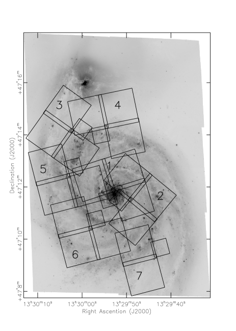
Figure 1: Footprints of the WFPC2 $U_{F336W}$ fields used in this study, overlaid on the ACS $B_{F435W}$ mosaic image. The numbers refer to the different datasets in Table 1.

Table 1: Overview of the different HST/WFPC2 $U_{F336W}$ band datasets used in this study.

Fielda	ID	PI	Dataset (association)	Exposure time	Observation date
1	5652	R. P. Kirshner	U2EW0205B	$3\times 400=1200$ s	12 May 1994
2	7375	N. Scoville	U50Q0105B	$2\times 600=1200$ s	21 Jul 1999
3			U9GA0201B	$2\times 1300=2600$ s	24 Jan 2006
4			U9GA5301B	$2\times 1200=2400$ s	28 May 2006
5	10501	R. Chandar	U9GA0401B	$2\times 1300=2600$ s	13 Nov 2005
6			U9GA0501B	$2\times 1300=2600$ s	13 Nov 2005
7			U9GA0601B	$2\times 1300=2600$ s	13 Nov 2005
a The numbers refer to the footprints in Fig. 1.

We used the individual chips (WF and PC) of the standard pipeline-reduced associations, i.e. no further data reduction was performed. On every chip between 6–11 sources were matched with sources on the ACS $B_{F435W}$ image. Using these sources the coordinate transformations between the WFPC2 chips and the ACS frame were calculated using the IRAF task geomap. The task geoxytran was used to transform the coordinates of the 7698 resolved sources of S07 on the ACS $B_{F435W}$ image to the WFPC2 chips. In most cases the root-mean-square accuracy in X and Y was better than one pixel, and in all cases better than 2 pixels.

Aperture photometry was performed at the transformed coordinates using DAOPHOT, allowing for a maximum centring shift of three pixels. For the PC chips a $(5,10,3)$ configuration was used for the radius of respectively the aperture, annulus and width of the annulus in pixels. For the WF chips the configuration was $(3,7,3)$. Aperture corrections to an aperture of 0.5″were measured using analytic cluster profiles with an effective radius of 3 pc, which were subsequently convolved with the PSF. These corrections for the WF and PC chips were $-0.14$ and $-0.19$ mag for the WF and PC chips, respectively. Zeropoints (calibrated for the 0.5″aperture) and CTE loss corrections were calculated following Dolphin (2000). We corrected for Galactic foreground extinction in the direction of M 51 according to Appendix B of Schlegel et al. (1998).

From the initial source list of 7698 resolved sources on the ACS $B_{F435W}$ image, we retrieved positive photometry on the WFPC2 $U_{F336W}$ images of 5502 sources. The remaining sources had either an aperture covering the edge of an image, a failure in daophot’s centring algorithm or a negative flux, caused by a combination of a faint source and noise in the background annulus. As can be seen in Fig. 1, there is some overlap between different WFPC2 chips. If a source had photometry in more than one $U_{F336W}$ chip, the photometry with the smallest error was selected.

In Fig. 2 we show the resulting photometry and error in the photometry for the $U_{F336W}$ passband. As expected, the photometry of fields 1 and 2 has larger errors compared to the photometry of fields 3–7, due to the deeper exposures of the latter fields. The horizontal line at $\sigma(\mbox{$U_{F336W}$})=0.2$ mag indicates the limit we applied to select only clusters with accurate photometry. The bin centred on $\mbox{$U_{F336W}$}=22$ mag indicates the magnitude at which approximately 10% of the clusters will be rejected from the sample by this $\sigma(\mbox{$U_{F336W}$})<0.2$ mag criterion. These limits will be used in Sect. 3.3 to select cluster samples.

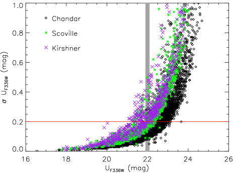
Figure 2: The error in the $U_{F336W}$ magnitude versus the $U_{F336W}$ magnitude for all 5502 sources for which we have photometry. The different symbols/colours refer to the different datasets listed in Table 1. The horizontal line indicates $\sigma\mbox{$U_{F336W}$}=0.2$ mag and the bin at $\mbox{$U_{F336W}$}=22$ mag indicates the magnitude range in which $\sim$90% of the clusters has $\sigma\mbox{$U_{F336W}$}<0.2$ mag.

3 Selection of the cluster samples

In this study we are primarily interested in the spatial distribution of young star clusters in the disc of M 51. We therefore used Simple Stellar Population (SSP) models to estimate the age, mass and extinction of all 5502 clusters for which we have $UBVI$ photometry (Sect. 3.1). The estimated ages were then used to select cluster samples with different ages (Sect. 3.3).

3.1 SSP model fitting

For our age determinations we used the galev SSP models (Schulz et al. 2002; Anders & Fritze-v. Alvensleven 2003) together with the analysed tool (Anders et al. 2004). In summary, analysed compares the broad-band spectral energy distribution (SED, in our case UBVI) of every cluster to a large grid of modelled SEDs for different ages, extinctions and metallicities. The model with the lowest $\chi^{2}$ is selected, and the (initial) mass of the cluster is derived by scaling the entire modelled SED to the observed SED. The models and the tool have been extensively tested (e.g. Anders et al. 2004; de Grijs et al. 2005; de Grijs & Anders 2006) and the uncertainty in the derived ages is typically $<0.4$ dex.

The galev models were preferred above other SSP models because of their freedom in stellar evolutionary models and metallicity and because their output and treatment of extinction is tailored to our specific HST/ACS filters. Therefore, no transformation between different photometric systems was necessary. We used the models based on the Geneva isochrones (Charbonnel et al. 1993; Schaerer et al. 1993), which are better suited for the age range we are interested in (i.e. age $\lesssim 100$ Myr) than e.g. Padova isochrones (Bertelli et al. 1994; Girardi et al. 2000), due to a higher time resolution in this age range. However, in Sect. 3.2 we will discuss the impact of the different isochrones on the derived cluster ages. For the models we further adopted a Kroupa (2001) stellar initial mass function (IMF) down to $0.1\mbox{$M_{\odot}$}$ and a metallicity between $0.4\mbox{$Z_{\odot}$}$ and $2.5\mbox{$Z_{\odot}$}$. This range in metallicity covers the observed metallicity of H II regions in the disc of M 51 (solar to twice solar, Diaz et al. 1991; Hill et al. 1997) and the slightly lower metallicity expected for older clusters. The extinction was varied between $0\leq\mbox{$E(B\!-\!V)$}\leq 1$ in steps of 0.05 and the Cardelli et al. (1989) extinction law was applied. Absolute magnitudes of all the clusters were calculated assuming $m-M=29.62$ (i.e. a distance to M 51 of $8.4\pm 0.6$ Mpc, Feldmeier et al. 1997). In Fig. 3 we compare the photometry of our clusters to the SSP models in two colour-colour diagrams.

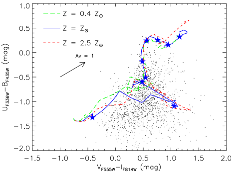
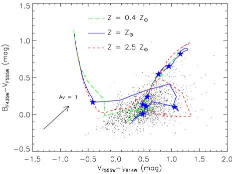
Figure 3: $\mbox{$U_{F336W}$}-\mbox{$B_{F435W}$}$ versus $\mbox{$V_{F555W}$}-\mbox{$I_{F814W}$}$ diagram (left) and $\mbox{$B_{F435W}$}-\mbox{$V_{F555W}$}$ versus $\mbox{$V_{F555W}$}-\mbox{$I_{F814W}$}$ diagram (right) of the 1580 clusters selected in Sect. 3.3 (not corrected for extinction), compared to galev SSP models using Geneva isochrones, a Kroupa IMF and three different metallicities, indicated in the figures. The stars indicated log(age/yr), starting from 6.6 (left) to 9.8 (top right) in steps of 0.4 dex.

3.2 Systematic uncertainties

Due to either the discreteness of the model isochrones or the rapid colour evolution of the models at certain ages in combination with the photometric uncertainties of the data, some fitting artefacts, or “chimney’s” will generally appear in the log(mass) vs. log(age) plane of the clusters (Bastian et al. 2005a; Gieles et al. 2005). We find that these artefacts depend on the SSP model parameters such as the adopted isochrones and the range in metallicity. In Fig. 4 we compare the ages of clusters fitted with our adopted parameters (Geneva isochrones, Z free between $0.4\mbox{$Z_{\odot}$}$ – $2.5\mbox{$Z_{\odot}$}$) to the ages fitted with metallicity fixed to solar or using Padova isochrones.

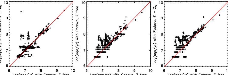
Figure 4: Comparison of cluster ages determined using different galev SSP model parameters, for the 1580 clusters selected in Sect. 3.3. The line shows the one-to-one correlation. Left: Geneva isochrones for solar metallicity versus Geneva isochrones for $\mbox{$Z_{\odot}$}<Z<2.5\mbox{$Z_{\odot}$}$. Middle: Padova isochrones versus Geneva isochrones, both for $\mbox{$Z_{\odot}$}<Z<2.5\mbox{$Z_{\odot}$}$. Right: Padova isochrones for solar metallicity versus Geneva isochrones for $\mbox{$Z_{\odot}$}<Z<2.5\mbox{$Z_{\odot}$}$.

First of all, Fig. 4 (left) shows that restricting the metallicity to be solar, leads to a more discrete distribution of ages and the exchange of clusters between the different chimney’s: many clusters from the $\log(\mathrm{age/yr})=7.2$ chimney (on the x-axis) are now fitted with log(age/yr) between 7.6–8 or around 6.7 (on the y-axis), i.e. they show a vertical scatter. Similarly, many clusters from the range $\log(\mathrm{age/yr})=6.7$–8.0 (x-axis) end up in the $\log(\mathrm{age/yr})=7.2$ chimney (y-axis), representing the horizontal scatter.

Secondly, Fig. 4 (middle & right) shows that with the Padova isochrones we generally fit older cluster ages for $\log(\mathrm{age})\la 7.5$ (x-axis). These panels also show the limited time resolution of the galev models based on Padova isochrones, in the first $\sim 16$ Myr. This is caused by the fact that in the galev models the resolution can only be as high as the lowest possible age, which is 4 Myr when using the Padova isochrones. The preference of Geneva based models for younger ages is likely a combination of a stronger contribution from red supergiants, leading to redder colours, and the higher age resolution, which lead to less “smoothing” of the colour fluctuations compared to the Padova based models.

We conclude from Fig. 4 that cluster age determinations based on UBVI broad-band photometry can be very uncertain in the first $\sim 100$ Myr due to the uncertainties in the adopted model parameters. These uncertainties will translate into uncertainties in the different age samples, which we will select in Sect. 3.3. Although we will use the ages based on the models using Geneva isochrones and $0.4\mbox{$Z_{\odot}$}<Z<2.5\mbox{$Z_{\odot}$}$ as our “standard ages” in the remainder of this work, we will check, when necessary, how robust our results are against using the other models of Fig. 4.

3.3 Selection of the different age samples

After fitting the SSP models to our sample of 5502 clusters with $UBVI$ photometry, we applied the following selection criteria to reject clusters with unreliable fits and to minimize incompleteness effects:

1. Photometry in $B_{F435W}$, $V_{F555W}$ and $I_{F814W}$ brighter than the 90% magnitude completeness limits determined by S07 for a source with an effective (half-light) radius of 3 pc in a high background region (respectively 24.2, 23.8 and 22.7 mag).

2. Photometric accuracy in $B_{F435W}$, $V_{F555W}$, $I_{F814W}$ and $U_{F336W}$ better than 0.2 mag.

These two criteria reduced our cluster sample from 5502 to 2089 clusters. Since the $U_{F336W}$ imaging was not part of the source detection, we do not have a well defined completeness limit in the $U_{F336W}$ passband. We can, however, make a rough estimate of the 90% completeness limit in $U_{F336W}$, since we performed the $U_{F336W}$ aperture photometry at the coordinates of all the resolved clusters on the $B_{F435W}$ image. This photometry was followed by the $\sigma\mbox{$U_{F336W}$}<0.2$ mag criterion. Using bins of $0.2$ mag wide, we measured that the magnitude at which this $\sigma\mbox{$U_{F336W}$}$ criterion recovers $\sim$90% of the clusters from the total sample is $\mbox{$U_{F336W}$}=22.0$ (see also Fig. 2). This magnitude can be considered as a rough estimate of the $U_{F336W}$ 90% completeness limit, since in a real completeness test the recovered fraction is measured as a function of the input magnitude and not of the measured (possibly extincted) magnitude. Also, in a proper completeness test the recovered clusters are compared to an input sample which is (by definition) 100% complete. In our case we can only measure the effect of the $\sigma\mbox{$U_{F336W}$}$ criterion on the detected sample, which is probably already affected by some incompleteness due to extinction. Keeping this in mind, we used the estimated $U_{F336W}$ limit as an extra criterion to select our cluster samples:

1. $\mbox{$U_{F336W}$}<22.0$ mag,

which further reduced our sample to 1580 clusters.

To estimate the impact of an extinction induced bias, we can do the following: if we would assume that $\mbox{$U_{F336W}$}=22.0$ mag is the detection limit for extinction free sources, we could correct the measured $U_{F336W}$ photometry of every source according to their best-fitting extinction, before applying the magnitude cut. This would include another 271 clusters in our sample. Still, such a correction would not account for the most extincted sources, which are not detected in the first place. This shows that extinction effects can introduce biases of the order of $\sim 15$% of the sample size. Unfortunately we have to accept that we simply can not fully correct for such extinction effects by the proper choice of magnitude cuts.

The extinction distribution is shown in Fig. 5 and is in excellent agreement with the results of Bik et al. (2003). Since the distribution is peaked towards low extinctions, most of the extra clusters, if we could correct for extinction, would be located close to the $U_{F336W}$ detection limit. We therefore note that, although one can use 90% completeness limits, since extinction (and also crowding, see e.g. S07) can not properly be taken into account, one will always end up with a sample being less than 90% complete. This also holds for the remainder of this work, where we nevertheless will use terms like “90% complete” for the sake of simplicity.

Figure 5: Distribution of the best-fitting extinctions ($E(B\!-\!V)$) of the 5502 clusters for which we have UBVI photometry.

The age-mass diagram for the clusters fullfilling criteria 1–3, is shown in Fig. 6. In this diagram two trends are immediately visible. First, we see that the mass of the most massive cluster generally increases with age. This is most likely a statistical size-of-sample effect caused by the logarithmic age interval (see e.g. Hunter et al. 2003; Gieles & Bastian 2008). Second, we see that the mass of the least massive clusters increases steadily with age. This is a selection effect caused by the detection limit (i.e. the most limiting 90% magnitude completeness limit, see criterium 1 above). For the $BVI$ passbands we also plotted the mass evolution with age, corresponding to the 90% magnitude completeness limit. For the $U_{F336W}$ passband we plotted the corresponding mass evolution for the applied $\mbox{$U_{F336W}$}=22.0$ limit. We see that for log(age/yr)$>6.7$ $U_{F336W}$ is the most limiting factor that sets the lower mass limit. These mass evolution curves were calculated using galev models with solar metallicity. The slope of these detection limits is caused by the evolutionary fading of the clusters: a less massive cluster reaches a constant magnitude limit much faster compared to a more massive cluster. These curves show that after $\sim 20$ Myr the limiting mass in $U_{F336W}$ evolves faster with age compared to the other passbands, because the integrated flux in $U_{F336W}$ is always dominated by the hottest (and therefore fastest evolving) stars. We see some clusters with best-fitted masses below the predicted limiting $U_{F336W}$ mass. This is possible because of two effects. First of all, the mass of a cluster is determined by scaling of the complete modelled SED (i.e. $UBVI$) and not by scaling a single passband only. Secondly, the curve for the limiting mass is for solar metallicity, while the best-fitting model can have a different metallicity.

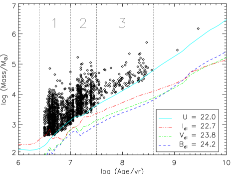
Figure 6: Log(mass) versus log(age) diagram of the 1580 clusters with photometric accuracies $<0.2$ mag and extinction corrected magnitudes brighter than the 90% completeness limits in $B_{F435W}$, $V_{F555W}$ and $I_{F814W}$ and $\mbox{$U_{F336W}$}<22.0$, as indicated in the lower-right corner. The corresponding mass limits as a function of age are indicated by the coloured lines. Note that the masses are initial masses (i.e. corrected for stellar evolution but not for secular evolution). The three magnitude-limited age samples are indicated by the numbered regions.

We selected three magnitude-limited cluster samples with different ages for the remainder of this study:

• Sample 1:
  $6.4\leqslant\mathrm{log(age/yr)}<7.0$
  Number of clusters: 895

• Sample 2:
  $7.0\leqslant\mathrm{log(age/yr)}<7.5$
  Number of clusters: 556

• Sample 3:
  $7.5\leqslant\mathrm{log(age/yr)}<8.6$
  Number of clusters: 127

These three cluster samples are indicated by the numbered regions in Fig. 6. The total number of clusters in these three samples is 1578.

Due to the systematic effects described in Sect. 3.2, our cluster samples will change significantly if we adopt the Padova stellar isochrones instead of the Geneva isochrones. This results in $\sim 230$ clusters less in sample 1, and $\sim 200$ clusters more in sample 3.

As can be seen from Fig. 6, our cluster samples have different lower-mass limits. Our youngest cluster sample contains clusters down to estimated masses of log($M/\mbox{$M_{\odot}$}$)$\approx 2.6$, but is 90% complete down to $\log(M/\mbox{$M_{\odot}$})=3.1$, while the lowest possible mass in our oldest cluster sample is log($M/\mbox{$M_{\odot}$}$)$\approx 3.7$. An electronic table with the photometry, ages, masses and extinctions of the clusters will be published together with a forthcoming paper (Scheepmaker et al. 2009).

4 Star formation rates, gas densities and spiral arms

4.1 Spiral arms

In order to study the relation between star and cluster formation and spiral structure, we first defined the two spiral arms in M 51 using data from the Two Micron All Sky Survey (2MASS), which we downloaded from the NASA/IPAC Extragalactic Database (NED). The background subtracted $H$-band (1.65$\mu$m) image was used, which is part of the 2MASS Large Galaxy Atlas (Jarrett et al. 2003). We used near-infrared data to trace the spiral arms, since the near-infrared is most sensitive to older stellar populations. This means that we are tracing the dominant mass component in the disc of M 51, independent of the dominant flux in the near-UV and optical of young star clusters and massive star formation.

We enhanced the spiral structure by first masking the companion galaxy, the inner 750 pc region, bright point sources and negative pixels. We then subtracted radial averages and convolved the resulting image with a Gaussian kernel with a FWHM of $25\arcsec$ ($\approx 1\leavevmode\nobreak\ kpc$). In the resulting smoothed image we identified 23 peaks tracing the two spiral arms using IRAF/DAOPHOT, and transformed their positions into polar coordinates. Finally, the regions in between the peaks were interpolated using cubic splines of the form $\ln(R(\theta))$. The resulting interpolated spiral arms are shown in Fig. 7, overplotted on the original background subtracted $H$-band image (left) and the enhanced image (right). We will refer to the arm extending towards the south-west (i.e. bottom-right) as “Spiral arm 1”, and to the arm extending towards the nort-east (top-left) as “Spiral arm 2”, as indicated in the figure.

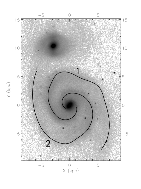
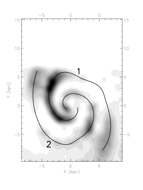
Figure 7: Left: Location of the two spiral arms, overlaid on the 2MASS Large Galaxy Atlas $H$-band image of M 51. The few black points are foreground stars. Right: Same spiral arms, overlaid on the enhanced (masked, radial average subtracted and smoothed) image.

4.2 Star formation rates and gas surface densities

In a recent paper Kennicutt et al. (2007, from here on referred to as “K07”) studied the locally resolved SFRs and gas densities in M 51, based on H$\alpha$, Pa$\alpha$, CO, H I and Spitzer Space Telescope 24$\mu$m imaging. For a series of 257 circular apertures with a diameter of $13\arcsec$ (corresponding to $\sim$530 pc) and distributed across the disc of M 51, these authors present extinction corrected SFR surface densities, as well as hydrogen gas and total gas surface densities. The SFRs are derived from the H$\alpha$ line emission (after extinction correction using Pa$\alpha$) using the transformation from Kennicutt (1998a), and are therefore tracing the current star formation up to $\sim$10 Myr (Calzetti et al. 2005). We used Table 1 of K07 to retrieve their list of aperture positions and the corresponding SFR surface densities and total gas surface densities.

The aperture positions were transformed to the frame of the ACS $V_{F555W}$ image using the IRAF task rd2xy. In Fig. 8 (left) we show the resulting positions of the $13\arcsec$ apertures. The mean SFR surface density in every aperture is indicated in greyscale. In the regions where two or more apertures are overlapping the average value was used.

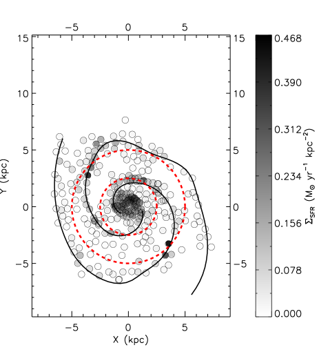
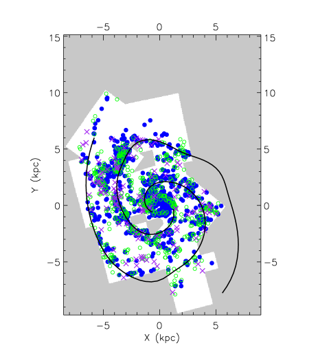
Figure 8: Left: Locations of the Kennicutt et al. (2007) $13\arcsec$ apertures used to trace the SFR and gas surface density in M 51. The greyscale indicates the mean SFR surface density. The spiral arms from Fig 7 are overplotted for reference. The two dashed circles are centred on the nucleus of M 51 and have a radius of 2.5 and 5 kpc, respectively. Right: Distribution of the cluster samples with different ages across the disc of M 51, in the same scale as the figure on the left. Filled blue (greyscale: black) circles: clusters with log(age/yr)$<7.0$. Open green (light grey) circles: clusters with $7.0\leqslant$ log(age/yr) $<7.5$. Purple (dark grey) crosses: clusters with $7.5\leqslant$ log(age/yr) $<8.6$. The regions not covered by the WFPC2 fields, i.e. for which we have no age estimation of the clusters, are indicated in grey. The spiral arms from Fig 7 are overplotted for reference.

5 Spatial distribution of star clusters and star formation

In Fig. 8 (right) we show the 2-dimensional spatial distribution of the three cluster samples in M 51. Also shown are the interpolated spiral arms from Fig. 7 and the regions (white) which are covered by the WFPC2 pointings, i.e. the regions for which we have derived ages of the clusters.

We can see from Fig. 8 that most current star formation is taking place in the centre of M 51 and at a galactocentric radius of $\sim 5$ kpc, and that these are also the locations where most of the young star clusters reside. We study these correlations more closely in Sect. 5.1 with the help of radial distributions.

Fig. 8 shows clearly that the majority of the clusters is closely tracing the spiral arms. This is expected, since the majority of the clusters are believed to be formed by the passing spiral density wave. Older clusters are expected to trace the spiral arms less closely, and we indeed see that the clusters from sample 3 ($\mathrm{log(age/yr)}\geqslant 7.5$) are more uniformly distributed. This is consistent with the result of Hwang & Lee (2008), who found that, using only the ACS $BVI$ data, the bluest clusters in M 51 are closely associated with the spiral structure and redder clusters are more uniformly distributed. We look at this in more detail in Sect. 5.2 using azimuthal distance distributions.

East (left) of the centre of M 51 the clusters are more concentrated on the convex (outward) side of spiral arm 1 compared to the concave (inward) side, up to $\sim$5 kpc. For spiral arm 2 in the south-west this effect is less obvious, although we note that for spiral arm 2 we are much more hampered by selection effects due to the incomplete WFPC2 coverage.

Fig. 8 also shows that the distribution of clusters itself is “clustered” in so-called cluster complexes (see e.g. Efremov 1995; Bastian et al. 2005b). These complexes are the largest groups in the hierarchy of star formation, which originates from the fractal distribution of the interstellar gas (Elmegreen & Efremov 1996; Efremov & Elmegreen 1998; Elmegreen & Elmegreen 2001). In such a hierarchy, the smallest observed structures are the youngest ones. This trend is visible in Fig. 8, were the spatial distribution of the youngest cluster sample shows most clustering and the amount of clustering decreases with the age of the cluster sample. We will quantify this more precisely in Sect. 5.3 with the help of two-point autocorrelation functions.

5.1 Radial distributions

From the 2-dimensional spatial distributions of SFR, gas surface densities and star clusters (Fig. 8) we derived radial density distributions using $13\arcsec$ wide circular annuli and, in case of the clusters, masking out the regions not covered by the WFPC2 fields (i.e. the grey area in Fig. 8 (right)). The SFR and gas apertures cover the entire field of view, so no masking was necessary for those. In Fig. 9 we compare the radial number density distributions of the different cluster samples directly to the SFR surface density distribution. Fig. 10 shows the radial distribution of the total gas surface density (including helium and metals), and in Fig. 11 we show the radial surface brightness distributions of the older stellar populations (no masking applied), derived from 2MASS $J$, $H$ and $K$-band imaging (Jarrett et al. 2003). In a recent paper, Schuster et al. (2007) also presented radial distributions of SFR and gas density in M 51 using 20 cm radio continuum data for the SFR density and a combination of CO and H I data for the gas density. These distributions can be used as an independent check to the data taken from K07 and are also shown in Figs. 9 & 10. We note that Schuster et al. (2007) have corrected their distributions (i.e. the galactocentric radii) for the inclination angle of the disc of M 51, while the cluster densities and the densities from K07 have only been divided by an additional factor of 1.07 to correct for the effect of the inclination on the projected area of the apertures/annuli. With an inclination angle of only $20\,^{\circ}$ (Tully 1974), however, this difference is negligible for our purposes. Figures 9 & 10 show that the Schuster et al. (2007) distributions are smoother than the K07 distributions. This is consistent with the radio data having a lower resolution (namely a half power beamwidth of $15\arcsec$ for the SFR data and $13\arcsec$ for the gas data, compared to the $13\arcsec$ apertures of K07). The offset in the gas surface densities (Fig. 10) between K07 and Schuster et al. (2007) is probably due to differences in the conversion factors used to calculate the ${\rm H}_{2}$ column density based on the CO data.

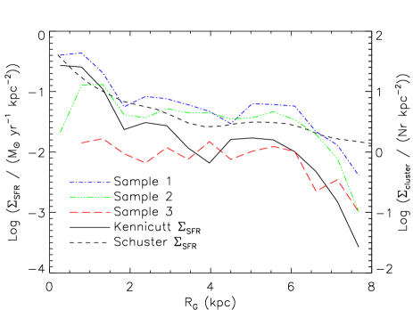
Figure 9: Radial number density distributions of the different cluster samples (right axis), compared to the radial distribution of the SFR surface density from Kennicutt et al. (2007) and Schuster et al. (2007) (left axis).

Figure 10: Radial distributions of the total gas (i.e. including helium and metals) surface density. The solid curve is derived from the data of Kennicutt et al. (2007), while the dashed curve is from Fig. 4 of Schuster et al. (2007).

Figure 11: Surface brightness distribution of M 51 in the 2MASS $J$, $H$ and $K$-band.

From Fig. 9 & 10 we see that both the SFR and gas density are peaking in the centre, and show two other distinct peaks at $\sim$2.5 and $\sim$5 kpc. These peaks are not simply a side effect of tracing a larger part of the spiral arms at these distances, as they are not clearly visible in the $K$-band surface brightness distribution (Fig. 11), while this band was used to define the spiral arms (Sect. 4.1). The locations of the peaks however, coincide with the locations of the four most active star forming regions in the spiral arms of M 51, as can be seen in Fig. 8 (left).

We see from Fig. 9 that the radial distribution of clusters younger than 10 Myr (sample 1) follows the SFR density distribution to a high degree (including the 2 peaks). Sample 2 shows a much flatter distribution but is still peaking towards the centre, followed by a dip within the inner $\sim$1 kpc, while the oldest cluster sample (sample 3) shows a flat distribution. These conclusions hold if we would use the Padova isochrones, and it agrees very well with the results of Hwang & Lee (2008), who find peaks at $\sim$3 and $\sim$6 kpc in the radial distribution of their “class 2” clusters (i.e. clusters which are more distorted and/or have multiple neighbours) and an increasing flattening of the radial distribution with increasing cluster colour (i.e. with increasing age, although some of their reddest clusters might be very young and extincted).

The peaks in $\Sigma_{\mathrm{SFR}}$, $\Sigma_{\mathrm{gas}}$ and $\Sigma_{\mathrm{cluster}}$ at $R_{\mathrm{G}}\approx 5$ kpc are consistent with an enhanced star formation activity caused by corotation (Elmegreen et al. 1989), since the corotation radius of M 51 is at $R_{\mathrm{G}}=5.4$ kpc, assuming a circular velocity of $V=200\mathrm{km}\,\mathrm{s}^{-1}$ (García-Burillo et al. 1993) and a pattern speed of $\Omega_{\mathrm{p}}=37\mathrm{km}\,\mathrm{s}^{-1}\mathrm{kpc}^{-1}$ (Zimmer et al. 2004). The peaks at $R_{\mathrm{G}}\approx 2.5$ kpc could be explained by the presence of the 4:1 resonance, which is were $\Omega-\kappa/4$ equals the pattern speed, $\Omega$ being the angular velocity of the stars and interstellar material and $\kappa$ the epicyclic frequency (Contopoulos & Grosbøl 1986, 1988). Elmegreen et al. (1989) have found evidence for a spiral arm amplitude minimum at this resonance, consistent with the gaps, orbital loops and stellar orbit crowding, that are expected for this resonance (Contopoulos & Grosbøl 1986). It is also suggested that orbit crowding and loops result in more gas shocking. This would lead to enhanced star formation at the 4:1 resonance radius, resulting in an enhancement of $\Sigma_{\mathrm{SFR}}$ at $\sim$2.5 kpc, which is then followed by an enhanced $\Sigma_{\mathrm{cluster}}$ for the youngest cluster sample.

5.2 Azimuthal distributions

If the formation of star clusters is triggered by gas shocking due to the passing spiral density wave (Roberts 1969), we expect the youngest star clusters to be located closer to the spiral arms compared to older clusters. Using the spiral arms from Fig. 7, we derived for every cluster their azimuthal distance from their closest spiral arm, assuming circular orbits. No corrections for the position angle (PA) and inclination angle ($i$) were applied, since these will practically be negligible for the almost face-on orientation of M 51 ($\mathrm{PA}=170\degr$, $i=20\degr$, Tully 1974). In Fig. 12 we show the distribution of the azimuthal distances for the three cluster samples (sometimes referred to as the “circular distribution”, e.g. Boeshaar & Hodge (1977)), normalized by the total number of clusters in every sample. The figure shows that all cluster samples are peaking at the location of the spiral arms (i.e. an azimuthal distance of $0\degr$). Although the youngest clusters (sample 1) show the most smooth distribution (i.e. with less scatter) compared to the other two samples, K-S tests do not indicate statistically significant differences between the samples. This result is robust against the variations of the SSP model parameters, used to derive the cluster ages, as described in Sect. 3.2.

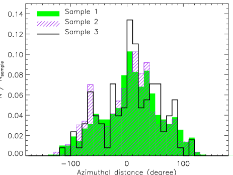
Figure 12: Normalized distribution of the azimuthal distance of the clusters to their closest spiral arm.

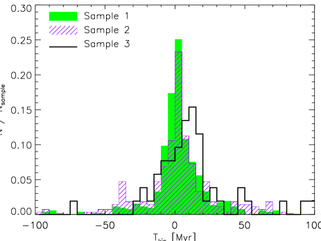
Figure 13: Normalized distribution of the kinematic ages of the clusters from their closest spiral arm, for the clusters with a galactocentric distance $<4$ kpc.

The fact that the oldest cluster sample is peaking at the centre of the spiral arms is likely a side effect of the enhanced cluster formation around the co-rotation radius (Sect. 5.1). Around the co-rotation radius the drift velocity away from the spiral arms is very low, meaning that older clusters once formed in these regions are still located close to the arms. The azimuthal distance of the clusters from the spiral arms expressed in terms of “kinematic age” will therefore be a better description of the differences in the circular distributions between the three cluster samples. In Fig. 13 we show the circular distributions in units of kinematic age, $T_{\mathrm{kin}}$, which is the azimuthal distance to the closest spiral arm, divided by the local drift velocity at the location ($R_{\mathrm{G}}$) of the cluster. A negative $T_{\mathrm{kin}}$ implies that the cluster is still approaching its closest spiral arm. In Fig. 13 we only plotted clusters with $R_{\mathrm{G}}<4$ kpc, i.e. well within the co-rotation radius, since close to co-rotation $T_{\mathrm{kin}}$ will diverge and outside the co-rotation radius the “kinks” or near-circularity of the spiral arms could make the intersection of the cluster orbit and spiral arm ambiguous. Note that this prescription for $T_{\mathrm{kin}}$ does not account for the passing of multiple spiral arm, e.g. an old cluster which has passed numerous spiral arms in its orbit can still be appointed a very low kinematic age, if it currently happens to be located close to an arm.

This notwithstanding, we see in Fig. 13 that the oldest cluster sample is peaking at older kinematic ages (10–15 Myr) compared to the younger two cluster samples, which peak at 0–5 Myr. We also see that sample 1 has a larger fraction of clusters at the youngest kinematic ages left of the peak compared to sample 2. The kinematic ages of the peaks in the distributions are younger than the typical ages of the clusters in the samples, indicating that the majority of the clusters formed $\sim 5$–20 Myr before their parental gas cloud would have reached the centre of the spiral arm. This is in agreement with the sharp edge of the dust clouds, seen on the HST/ACS image (see e.g. the dust lane covered by field 1 and 2 in Fig. 1). For a collapse time of the order of $10^{6}$ years we expect most contracting clouds to have formed a cluster well before the centre of the spiral arm is reached. Tamburro et al. (2008) find a timescale of 3.3 Myr in M 51 for the transition from H I emission, via CO emission to 24$\mu$m emission from current star formation. Since H I first has to condense to $\mathrm{H}_{2}$, the collapse time has to be shorter than 3.3 Myr.

The circular distributions are reasonably symmetrical around their peaks, which is consistent with the circular distributions found for H II regions in other spiral galaxies (e.g. in NGC 4321, Anderson et al. 1983) and it is in qualitative agreement with the density wave models which predict a more smoothed surface brightness distribution across spiral arms (e.g. Bash 1979), as opposed to the models which predict an asymmetric distribution (Roberts 1969).

5.3 Clustering of star clusters

The degree of clustering for different cluster samples can be quantified and compared by using the two-point correlation function (Peebles 1980, § 45). Applied to clusters from the same cluster sample, the two-point correlation function becomes an autocorrelation function. In the following, we broadly follow the method described in Peebles (1980) and Zhang et al. (2001). Zhang et al. applied two-point correlation functions to star clusters in NGC 4038/39 (the “Antennae”). The autocorrelation function is defined as:

$$1+\xi(r)=\frac{1}{\bar{n}N}\sum_{i=1}^{N}n_{i}(r),$$ (1)

where $n_{i}(r)$ is the number density of clusters found in an aperture of radius $r$ centred on, but excluding cluster $i$. $N$ is the total number of clusters and $\bar{n}$ is the average number density of clusters (excluding the grey regions in Fig. 8 (right)). In general, $\xi(r)$ is defined such that $\bar{n}[1+\xi(r)]\mathrm{d}V$ is the probability of finding a neighbouring cluster in a volume $\mathrm{d}V$ within a distance of $r$ from a random cluster in the sample (Peebles 1980). For our spatial distribution of clusters this means that $1+\xi(r)$ is a measure for the mean surface density within radius $r$ from a cluster, divided by the mean surface density of the total sample (i.e. the surface density enhancement within radius $r$ w.r.t. the global mean). Therefore, a random distribution of clusters will have a constant $1+\xi(r)=1$, while for a clustered distribution $1+\xi(r)>1$.

Since the star clusters in M 51 reside primarily in the disc, while the observations cover a larger projected area, all cluster samples will show some degree of autocorrelation and the absolute scaling of $1+\xi(r)$ will be arbitrary. We can, however, compare the relative scaling of $1+\xi(r)$ between the different cluster samples as well as the different functional forms.

In Fig. 14 we show the autocorrelation functions as a function of radius for the three cluster samples. Before the autocorrelation was calculated, the original ACS coordinates were mapped onto a new image with $1\arcsec$ resolution to reduce computing time. We took into account that as a result of this binning, one pixel could contain multiple clusters. For the errorbars we used (Peebles 1980, § 49):

$$\delta(r)=\left(\frac{1}{2}\sum_{i=1}^{N}n_{\mathrm{p}}(r)\right)^{-1/2},$$ (2)

where $n_{\mathrm{p}}(r)$ is the number of pairs formed with the central cluster $i$ of the current aperture, and the factor $1/2$ accounts for not counting every pair twice.

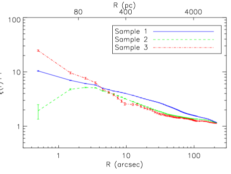
Figure 14: The autocorrelation function as function of radius for the three cluster samples.

Fig. 14 shows that for $r>4\arcsec$ ($\sim 160$ pc) the clusters with ages $<10$ Myr (sample 1) are most clustered (largest $\xi(r)$) and that the amount of clustering decreases with age. This is consistent with the visual interpretation of Fig. 8 (right). This result is robust against variations in the isochrones (Padova or Geneva) or metallicity range used in the SSP model fitting of our clusters. Below $r\sim 10\arcsec$ (i.e. $\sim 400$ pc) we see a steady increase in the clustering of sample 3, surpassing sample 1 below $r\sim 4\arcsec$. We also see that below this radius the amount of clustering for sample 2 decreases. However, if we would use the Padova isochrones we find that the autocorrelation function of sample 3 is much flatter, while the turnover of sample 2 decreases. Due to this degeneracy, we can not draw any firm conclusions on the age dependency of the autocorrelation function on scales below $\sim 4\arcsec$.

Moreover, on these smallest scales we can be biased by selection effects in the original sample selection of resolved sources of Scheepmaker et al. (2007). In this sample selection, sources with a neighbouring source within 5 ACS pixels (i.e. 0.25″) were rejected, possibly lowering the amount of autocorrelation in the first radius bin in Fig. 14. Crowding effects and the high background in the most compact regions in which the star clusters form, will also introduce a bias against the detection of clusters on the smallest scales. This bias will be stronger for younger clusters, since in a hierarchical (i.e. “scale free”) model of star formation the youngest structures are also the most compact ones. Correcting for such biases will increase the autocorrelation function of our youngest sample (sample 1), as we will show below.

The general trend of $1+\xi$ decreasing with radius is expected for hierarchical (i.e. “scale free” or “fractal”) star formation (e.g. Gomez et al. 1993; Larson 1995; Bate et al. 1998). If we consider a compact, isolated grouping of newly formed star clusters, we expect such grouping to disperse with a typical velocity dispersion $<10\leavevmode\nobreak\ \mathrm{km}\,\mathrm{s}^{-1}$ (Whitmore et al. 2005). For a 10 and 30 Myr old population of clusters, autocorrelation is therefore expected to increase on scales smaller than roughly 100 and 300 pc, respectively (which are lower limits, considering the initial size $>0$ pc of the GMC that formed the grouping). On larger scales, the autocorrelation for an isolated grouping of clusters is expected to level off. However, this will only hold if the grouping was not part of a larger hierarchy of star formation. In a hierarchical model, on the other hand, the clusters will be correlated with other clusters from other groupings on larger scales, together forming a group higher up in the hierarchy of star formation. The smooth decline of $1+\xi$ with radius, observed for our cluster samples on scales $r>3\arcsec$, is therefore consistent with these populations being part of this hierarchy. The velocity dispersion will cause an overall decrease of the amount of clustering of the star clusters with time (Bate et al. 1998), consistent with Fig. 14.

For a hierarchical, or fractal, distribution of stars or clusters, the autocorrelation function will show a powerlaw dependency with radius of the form $1+\xi(r)\propto r^{\eta}$ (Gomez et al. 1993). For such a distribution, the total number of clusters ($N$) within an aperture increase with radius as $N\propto r^{\eta}\cdot r^{2}=r^{\eta+2}$, which shows that $\eta$ is related to the (two-dimensional or projected) fractal dimension $D_{2}$ as $D_{2}=\eta+2$ (Mandelbrot 1983; Larson 1995). The distribution of star formation and interstellar gas over a large range of environments is observed to show a (three-dimensional) fractal dimension of $D_{3}\sim 2.3$ (e.g. Elmegreen & Falgarone 1996; Elmegreen & Elmegreen 2001) Projecting this three-dimensional fractal on a plane will result in a two-dimensional fractal dimension $D_{2}\approx D_{3}-1=1.3$ (Mandelbrot 1983; Beech 1992; Elmegreen & Elmegreen 2001). In the spiral galaxy NGC 628, Elmegreen et al. (2006) observe star-forming regions with $D_{2}=1.5$.

If we fit powerlaws to the straight parts of the autocorrelation functions in Fig. 14 ($4\arcsec<r<50\arcsec$), we find that the decreasing trend of sample 1 and 2 can be approximated with a power law index of around $-0.4$ (fractal $D_{2}=1.6$). Sample 3 has a lower index of around $-0.8$ ($D_{2}=1.2$), but as mentioned before, this index depends strongly on the stellar isochrones used: using the Padova isochrones, some clusters from sample 2 are fitted with older ages (see Fig. 4) and move to sample 3, flattening the autocorrelation function to a power law with an index of around $-0.4$. Interestingly, an index of $-0.4$ is similar to the index Zhang et al. (2001) find for candidate young stars in the Antennae galaxies (namely an index of $-0.41$), while the same authors find steeper slopes for the autocorrelation functions of young (5–160 Myr) star clusters (namely indices between $-0.74$ and $-1.06$). In an attempt to minimize the possible bias due to crowding of the youngest clusters, we also determined the autocorrelation function of all clusters in sample 1 with $\log(M/\mbox{$M_{\odot}$})>3.7$. This sample will have a higher completeness in the densest star forming regions. For this mass-limited sample we find a power law index of $-0.8$ ($D_{2}=1.2$, Geneva) or $-0.7$ ($D_{2}=1.3$, Padova), similar to the indices of Zhang et al. (2001) and consistent with the fractal dimension of $\sim 1.3$, mentioned above. This suggest that the flatter slope of the full sample 1 population of clusters is indeed biased, and that the unbiased index of the autocorrelation function of young clusters is similar for different galaxies. In other words, this hints towards a universal fractal dimension of hierarchical star formation. More studies in different galaxies and of different nature are necessary to strengthen this point.

5.4 Spatial correlation between star clusters and star formation

The crosscorrelation function (Eq. 1) can also be used to study the correlation between star clusters and the flux from any image. We can rewrite Eq. 1 as:

$$1+\xi(r)=\frac{1}{\bar{f}N}\sum_{i=1}^{N}f_{i}(r),$$ (3)

following Zhang et al. (2001, their Eq. 2), where $f_{i}(r)$ is now the intensity (i.e. flux per pixel) in an aperture with radius $r$ centred on cluster $i$, and $\bar{f}$ is the mean intensity over the whole image. For both the calculation of $f_{i}(r)$ and $\bar{f}$ the areas not covered by $U$-band imaging are masked out. To study the crosscorrelation between star clusters and star formation, we used the 20 cm radio continuum (RC) map (Patrikeev et al. 2006), and the HST/ACS H$\alpha$ mosaic image of M51 (Mutchler et al. 2005), which we continuum subtracted using a combination of the ACS $V_{F555W}$ and $I_{F814W}$ images. The 20 cm RC map was also used by Schuster et al. (2007) to derive the radial SFR distribution (shown in Fig. 9). The SFRs from the apertures of Kennicutt et al. (2007) (Fig. 8) are not suitable to be directly used in Eq. 3 due to their incomplete spatial sampling.

The 20 cm RC is tracing star formation through the synchrotron radiation coming from cosmic rays, emitted by supernovae explosions of massive stars. The exact relation between SFR and RC emission, however, is not well defined. It depends on the scaling between RC and far-infrared dust continuum emission, of which the general form and radial dependencies are still under debate (see e.g. Helou et al. 1985; Marsh & Helou 1995; Niklas & Beck 1997; Niklas 1997; Murgia et al. 2005; Murphy et al. 2006, 2008). For our current study, however, we are not interested in the exact scaling between RC or H$\alpha$ flux and SFR. We simply use the RC and H$\alpha$ flux to study how star clusters and two spatially complete tracers of star formation correlate for differently aged cluster samples.

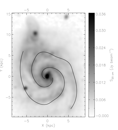
Figure 15: Radio continuum (20 cm) image of M 51, with the spiral arms of Fig. 7 overplotted for reference.

Before we applied the crosscorrelation function (Eq. 3) to the 20 cm RC image (shown in Fig. 15), the image was cropped to match the ACS mosaic frame and resampled to a pixel scale of $1\arcsec$ (the original image had a pixel scale of $2\arcsec$ and a beam size of $15\arcsec$). Due to computational issues the H$\alpha$ image, with a resolution of $0.05\arcsec$ was binned by a factor of 10 to a pixel scale of $0.5\arcsec$. For the uncertainty in $1+\xi(r)$ we again followed Zhang et al. (2001), adopting only the statistical uncertainty in the number of clusters per sample ($N$), leading to:

$$\delta(r)=N^{-1/2}(1+\xi(r)).$$ (4)

In Fig. 16 we show the resulting crosscorrelation functions between the three cluster samples and the RC flux. The crosscorrelation functions are flat on scales $<10\arcsec$, which is very likely a result of the beam size of the radio data. It is evident that the youngest cluster sample is most correlated (i.e. largest $\xi(r)$) with the RC emission on all scales smaller than $\sim 100\arcsec$ (i.e. $\sim 4$ kpc), and that the correlation drops with the age of the cluster population. A random distribution of clusters would have a constant $\xi(r)+1=1$. In other words, most of the radio flux is concentrated around the youngest clusters, as expected.

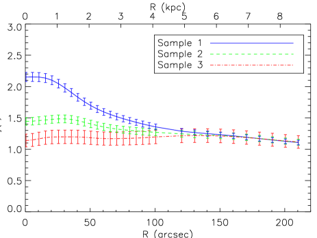
Figure 16: Crosscorrelation function between the three cluster samples and the 20 cm radio continuum image.

The crosscorrelation function between the 20 cm RC emission and the youngest cluster sample drops to half its peak value at $R\approx 2$ kpc. This shows that the RC emission is tracing star formation in a very diffuse way, consistent with the long path length of the cosmic rays, before they stop emitting RC emission.

In Fig. 17 we show the crosscorrelation functions between the three cluster samples and the (continuum subtracted) H$\alpha$ flux. The youngest clusters are strongly correlated to the H$\alpha$ flux. The correlation peaks at the resolution limit of $R=0.5\arcsec\approx 20$ pc and drops to half the peak value at $R\approx 100$ pc. This radius is consistent with the typical expansion speed ($\sim$10 $\mathrm{km}\,\mathrm{s}^{-1}$) of the ionized bubbles of hot stars (e.g. Lamers & Cassinelli 1999, p. 369). At a radius larger than the typical travel distance of an H$\alpha$ bubble in 10 Myr (i.e. $\sim$100 pc) the correlation is expected to level off. For sample 2 clusters the correlation with H$\alpha$ is considerably less and the sample 3 clusters shows a crosscorrelation function with H$\alpha$ consistent with a random distribution (i.e. $\xi(r)+1=1$, although a slight offset from 1 is expected due the large scale structure or M 51, see below).

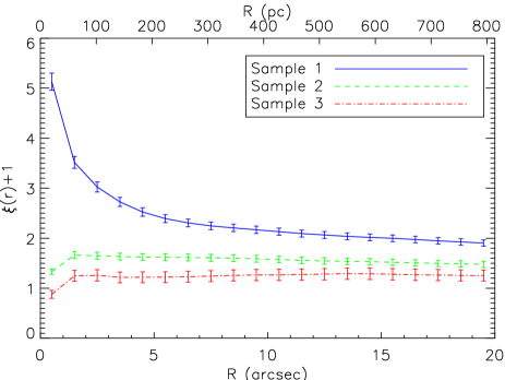
Figure 17: Crosscorrelation function between the three cluster samples and the (continuum subtracted) H$\alpha$ image. Note the difference in X- and Y-scaling compared to Figs. 16 & 18. On a larger scale, the three curves would converge to $\xi+1=1.1$ at $R\approx 120\arcsec\approx 5$ kpc, similarly to Fig. 16.

As a consistency check, we also derived the crosscorrelation functions between the star clusters and the flux from the 2MASS $H$-band image, which we used to define the spiral arms (Fig. 7). Since this near-infrared data is mostly tracing older stellar populations, no enhanced correlation with young star clusters is expected. In Fig. 18 the crosscorrelation functions are indeed shown to be indistinguishable. All three clusters samples, however, show an increased correlation towards smaller radii. This is likely an effect of the large scale structure of M 51. Both the cluster and $H$-band flux density are higher in the disc and spiral arms of M 51, while the observations (and thus the normalisation factor $\bar{f}$ in Eq. 3) cover a larger area. This leads to some degree of correlation towards smaller scales. The fact that this correlation is similar for all cluster ages confirms that the $H$-band flux is a good tracer of stellar density and not of current star formation.

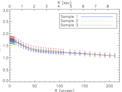
Figure 18: Crosscorrelation function between the three cluster samples and the 2MASS $H$-band image of M 51.

6 Summary and conclusions

We have studied the spatial correlations between star clusters and star formation across the spiral galaxy M 51. We combined published data of the resolved star formation law in M 51 (SFR and gas surface densities, Kennicutt et al. 2007) with the star cluster data of Scheepmaker et al. (2007). We combined the star cluster data with new HST/WFPC2 $U_{F336W}$ data of 1580 clusters in order to estimate ages, masses and extinctions of these clusters using SSP models. We used radial and azimuthal distributions and cross-correlation functions to study the spatial correlation between star formation, star clusters and spiral structure. We used auto-correlation functions to study how the clustering of star clusters depends on age and spatial scale. The main conclusions of this work can be summarized as follows:

1. We find that age determinations of young ($\lesssim 100$ Myr) star clusters based on broad-band UBVI photometry can depend strongly on the adopted stellar isochrones used in the SSP models. Using models based on the Padova isochrones, we generally find older, and therefore more massive, clusters compared to the same models based on the Geneva isochrones (Fig. 4).

2. The radially averaged distributions of star formation and gas surface density in M 51 peak in the centre and subsequently at $\sim 2.5$ and $\sim 5$ kpc. These distributions are matched by the number surface density distribution of our youngest star cluster sample (ages $<10$ Myr, Fig. 9), while for the older clusters the distributions are more flat. We note that the location of the peaks coincide approximately with the locations where the spiral arms meet the 4:1 resonance and the co-rotation radius.

3. The distributions of azimuthal distances from the spiral arms show that most of the young and old star clusters are located at the centre of the spiral arms, with the youngest star clusters showing the most smooth distribution (Fig. 12). In terms of kinematic age and for $R_{\mathrm{G}}<4$ kpc, the azimuthal distribution of the oldest clusters peaks at the largest separation downstream of the spiral arms (10–15 Myr), while the majority of the younger clusters are within 0–5 Myr downstream of the arms. This indicates that the majority of the clusters formed $\sim 5$–20 Myr before their parental gas cloud would have reached the centre of the spiral arm.

4. We find that the amount of clustering of star clusters decreases both with spatial scale and age (Fig. 14), consistent with hierarchical star formation. The slope of the autocorrelation functions of the youngest clusters ($\log(\mathrm{age})<7.5$) is consistent with a projected fractal dimension of 1.6. We find a lower fractal dimension of 1.2 for the clusters with $\log(\mathrm{age})<7.0$, if we use a higher mass limit and thus, for this smaller mass range, a more complete sample. On spatial scales smaller than 400 pc, the amount of clustering of the oldest cluster samples is very uncertain due to uncertainties in the assumed SSP model parameters.

5. The locations of the youngest star clusters are highly correlated with the flux from 20 cm radio-continuum emission and continuum subtracted H$\alpha$ emission, but not with near-infrared $H$-band emission. The correlation with the radio emission is more diffuse compared to the correlation with H$\alpha$, and both correlations decreases with the age of the cluster population.

In a follow-up paper (Scheepmaker et al. 2009) we will focus on the quantitative comparison between star and cluster formation, discussing the fraction of total star formation taking place in optically visible star clusters.