Electroweak symmetry breaking as a proximity effect

Abstract:

The proximity effect in condensed matter physics is a mechanism that naturally produces weak superconductivity. We argue that a braneworld can similarly produce a low-energy breaking of the electroweak symmetry, provided that in addition to the “normal” region, occupied by the conventional phase of QCD, there is a bulk region where the color is in an anisotropic (layered) state with a larger confinement scale. The $W$ and $Z$ bosons, as well as the quarks, acquire masses by scattering off the layered region. A peculiar feature of this scenario is that the strongly interacting sector responsible for the symmetry breaking can be much lighter than the conventional 1 TeV.

1 Introduction

The proximity effect in condensed matter physics is a mechanism by which a material becomes weakly superconducting when placed in the proximity of a conventional (“strong”) superconductor. Given the parallel between superconductivity and the electroweak symmetry breaking, one may wonder if a similar mechanism is at work also in the latter case.

A natural framework for exploring this possibility is anisotropic states of higher-dimensional lattice gauge theories. Perhaps the best known of these is the layer phase [1, 2, 3, 4, 5, 6], in which the gauge field is localized in $d$-dimensional layers, so that the charges within each layer interact according to the Coulomb law. The requirement that the Coulomb phase be present is the reason why for $d=4$ the genuine layer phase can exist only in Abelian gauge theories [1].

For our purposes, however, the Coulomb law is unnecessary and, indeed, detrimental. We are interested in the situation when the layers are confining, but the confinement (correlation) length within the layers is much larger than in the direction perpendicular to them. We do not require such states to form a separate phase; in fact, we expect them to be a corner of the usual confining phase of the higher-dimensional theory.

We refer to such a state as a layered state or a layered region, as opposed to a layer phase. In Sec. 2, we argue that for the ${\rm SU}(3)$ gauge group in $d+1=5$ dimensions it is separated from the weakly-coupled phase by a first-order phase transition.

Additional possibilities appear when the fifth dimension is appreciably curved, as in the case, for example, of a brane bounding space with a negative cosmological constant [7]. For ${\rm SU}(3)$, the resulting variation of the gauge coupling produces a weakly-coupled “normal” region near the brane and a layered region further away, with a well defined phase boundary between them. Because the length of the “normal” region (indeed, in our case, of the entire fifth dimension) is finite, we expect that at large 4-dimensional distances the 5-dimensional theory there reduces to its 4-dimensional counterpart. So, in this limit, both the “normal” and layered regions are confining, but with different confinement scales: in the “normal”region, the confinement scale is the usual $\Lambda_{\rm QCD}$, while in the layers it is a much larger $\Lambda$. We suggest that the quark condensates of the layered ${\rm SU}(3)$ color are the origin of the masses of the $W$ and $Z$ bosons.

The argument of Sec. 2 is based on the mean-field theory [8], which had been a reliable guide to the phase structure of anisotropic 5-dimensional Abelian theories [1, 2, 3, 4, 5, 6]. At the mean-field level, the “normal” phase is ordered, with respect to the link variable connecting individual 4-dimensional hyperplanes. In the non-Abelian case (with a finite fifth dimension), we expect that this order is destroyed by confinement, and in this sense the mean field is formally in error. However, if the mean-field phase transition is strongly first-order, and the confinement length is large, we do not expect the transition to disappear altogether. This is the rationale on which we proceed here.

Instead of a full 5-dimensional lattice, one could use deconstruction [9, 10]—the approach where one latticizes only the additional, fifth dimension or, in other words, considers multiple instances of the 4-dimensional theory connected to one another by sigma-model variables. These sigma-model variables correspond to the link variables $U_{\tilde{\alpha}}$ of the lattice gauge theory (${\tilde{\alpha}}$ labels the links). The simplest version of the proximity effect is realized when there is a first-order phase transition in the sigma model. If, as in the present case, $U_{\tilde{\alpha}}$ are elementary ${\rm SU}(3)$ fields living on the sites of a 4-dimensional lattice, there is evidence for such a transition already at the mean-field level [11]. We expect very similar physics in the case when the nonlinear sigma model is replaced with a linear one (i.e., $U_{\tilde{\alpha}}^{\dagger}U_{\tilde{\alpha}}$ is allowed to fluctuate), as in one version of deconstruction [9, 10]. In another version [9], $U_{\tilde{\alpha}}$ are composites of new confining gauge theories. To explain quark masses, we require that there are quark hopping terms, of the form $\bar{q}_{\alpha}U_{\tilde{\alpha}}q_{\alpha+1}$. The presence of such terms suggests that, if $U_{\tilde{\alpha}}$ are “mesons” of a new confining theory, the quarks must be “baryons,” meaning that they are also composite. This is a fascinating possibility, but also one more challenging to explore than the fully latticized theory considered here.

Our proposal can also be compared to Higgsless models [12, 13], where the electroweak symmetry is broken by boundary conditions in the extra dimension. Unlike the boundary conditions, the layered-state quark condensates deform the profiles of $W$ and $Z$ relatively little, provided the fifth dimension is sufficiently short. (These profiles are discussed further in Sec. 3.) As a result, no new gauge symmetries are required to avoid a large tree-level contribution to the ratio of the $W$ and $Z$ masses (the $\rho$ parameter).

Overall, we find that the layered-state color functions much like the conventional technicolor [14, 15, 16], with the following differences.

(i) The confinement scale $\Lambda$ of the layer theories does not have to be of order $v\sim 250$ GeV: because more than one layer can contribute to the $W$ mass, it can be much smaller than that. The masses of various new particles produced by the strongly coupled sector are then much smaller than the conventional 1 TeV. TeV-scale masses of new particles are a major reason why the conventional technicolor runs into conflict with the measured value of the $S$ parameter [17]. A lower confinement scale may improve prospects for obtaining an acceptable value (although we have not yet ascertained whether it actually does so).

(ii) Quarks acquire masses by scattering off the layered region (a process similar to Andreev reflection [18] in a superconductor-normal-superconductor junction). So, the problem of quark masses, which is quite formidable in the conventional technicolor, has a natural solution here.

(iii) The quark scattering off the layers can break flavor symmetries. This may help to lift the masses of pseudo-Goldstone bosons produced by chiral symmetry breaking in the layers to an acceptable level.

2 Layered states in five-dimensional gauge theories

Consider a background of the Randall-Sundrum type [7], with the line element

$$ds^{2}=dz^{2}+a^{2}(z)\eta_{\mu\nu}dx^{\mu}dx^{\nu}\equiv g_{MN}dx^{M}dx^{N}\,.$$ (1)

Greek indices run from 0 to 3, and $\eta_{\mu\nu}=\mbox{diag}(-1,1,1,1)$ is the Minkowski metric tensor. Similarly to Ref. [7], we consider an orbifolded $z$ direction, $z\in S^{1}/Z_{2}$, with two branes at the orbifold’s fixed points: one, near which we live, at $z=0$, where the warp factor $a(z)$ is maximal, and the other at $z=\pi R$. We do not, however, take $R$ to infinity, so the fifth dimension remains compact. A gauge field $A_{\mu}$ is assumed even under the orbifold group $Z_{2}$, $A_{5}$ odd; the orbifold projection of fermions will be defined in Sec. 4.

The naive continuum action of a 5-dimensional gauge theory is

$$S_{\rm cont}=-\frac{1}{4g_{5}^{2}}\int d^{4}xdz\sqrt{-g}g^{\mu\nu}\left(g^{\rho\sigma}G^{a}_{\mu\rho}G^{a}_{\nu\sigma}+2g^{zz}G^{a}_{\mu z}G^{a}_{\nu z}\right),$$ (2)

where $G^{a}_{\mu\rho}$ and $G^{a}_{\mu z}$ are the field strengths. The two terms in Eq. (2) contain different metric functions, which leads to an anisotropy of the gauge coupling.

There is a degree of arbitrariness in choosing the lattice discretization of Eq. (2). The choice matters: at large $z$, where the theory is in the layered state, the 4-dimensional hyperplanes decouple from each other, so we are dealing with a collection of individual 4-dimensional gauge theories. The inverse coupling constants of these theories are

$$\frac{1}{g_{4}^{2}}=\frac{\Delta z}{g_{5}^{2}}\;,$$ (3)

where $\Delta z$ is the lattice spacing in the $z$ direction. Here we discretize the imaginary-time version of Eq. (2) in such a way that both $\Delta z$ and $\Delta x$, the spacing in the $x^{\mu}$ directions, are independent of $z$. In this case, $g_{4}$ and the confinement scale $\Lambda$ of the 4-dimensional theories are also $z$-independent. We assume that $\Lambda\ll 1/\Delta x$, so that the layer theories are in the continuum limit. Then, at one loop,

$$\Lambda=\frac{1}{\Delta x}\exp\left\{-\frac{b}{g_{5}^{2}}\Delta z\right\}\;,$$ (4)

where $b$ is the coefficient of the one-loop beta-function.

In contrast to $g_{4}$, the usual coupling constant of QCD, $g_{\rm QCD}$, is determined by the “normal” region near the brane (see Fig. 1):

$$\frac{1}{g_{\rm QCD}^{2}}=\frac{z_{\rm eff}}{g_{5}^{2}}\;,$$ (5)

where $z_{\rm eff}$ is the effective length of that region (it may be different from the geometrical length due to effects at the phase boundary). If $z_{\rm eff}$ is sufficiently large in comparison with $\Delta z$, the confinement scale (4) is much larger than $\Lambda_{\rm QCD}$. So, when quarks are added, the chiral symmetry breaking in the layers will be correspondingly stronger. This is the basis of the proximity-effect scenario.

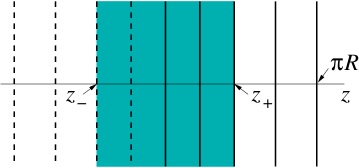
Figure 1: Arrangement of 4-dimensional hyperplanes along the $z$ direction. The dashed lines are hyperplanes obtained upon “unfolding” the orbifold, a convenience in the discussion of fermions in Sec. 4. The phase boundaries are at $z_{\pm}$. The shaded region is “normal”; the rest of the hyperplanes are in the layered state.

The imaginary-time lattice action corresponding to Eq. (2) is

$$S=-\sum_{\alpha,p}\beta_{\alpha}\chi(U_{\alpha,p})-\sum_{{\tilde{\alpha}},{\tilde{p}}}\beta^{\prime}_{\tilde{\alpha}}\chi(U_{{\tilde{\alpha}},{\tilde{p}}})\;.$$ (6)

The integer $\alpha$ labels different (4-dimensional) hyperplanes perpendicular to the $z$ axis, ${\tilde{\alpha}}$ labels the interval between $\alpha$ and $\alpha+1$, $p$ are plaquettes within a hyperplane, ${\tilde{p}}$ are plaquettes connecting the hyperplanes; $\chi(U)={\rm Tr}U$ for ${\rm SU}(n)$ (where the trace is taken in the fundamental representation), and $\chi(U)=\mbox{Re}U$ for ${\rm U}(1)$.

To simplify notation, we first write down the mean-field equations for the Abelian group ${\rm U}(1)$. These are similar to the equations obtained in Ref. [8] for the isotropic Abelian theory. Once the physics responsible for formation of the layer phase becomes apparent, we switch back to the non-Abelian case.

We seek to minimize the mean-field energy, whose 4-dimensional density (the potential) in the Abelian case is

$${\cal E}_{\rm mf}=-\sum_{\alpha}\left\{4[u(\Phi_{\alpha})-\Phi_{\alpha}u^{\prime}(\Phi_{\alpha})]+6\beta_{\alpha}[u^{\prime}(\Phi_{\alpha})]^{4}\right\}$$ (7)

$${}-\sum_{\tilde{\alpha}}\left\{u(\Phi_{\tilde{\alpha}})-\Phi_{\tilde{\alpha}}u^{\prime}(\Phi_{\tilde{\alpha}})+4\beta^{\prime}_{\tilde{\alpha}}\phi_{\alpha}\cdot\phi_{\alpha+1}u^{\prime}(\Phi_{\alpha})u^{\prime}(\Phi_{\alpha+1})[u^{\prime}(\Phi_{\tilde{\alpha}})]^{2}\right\}.$$

Here $\Phi_{\alpha}$ and $\Phi_{\tilde{\alpha}}$ are the mean fields conjugate, respectively, to the link variables $U_{\alpha\mu}$ and $U_{\tilde{\alpha}}$ and represented as two-dimensional vectors, $\phi_{\alpha}$ is the unit vector in the direction of $\Phi_{\alpha}$, a dot ($\cdot$) denotes the dot product of such vectors, and $u(\Phi)=\ln I_{0}(\Phi)$, where $I_{0}$ is the modified Bessel function. The numerical coefficients in Eq. (7) reflect the number of links (four) and plaquettes (six) per site of a 4-dimensional hyperplane.

Suppose that in the region of interest $\beta_{\alpha}$ is large, in comparison with both $\beta^{\prime}_{\tilde{\alpha}}$ and unity. Then, we can first minimize the in-plane potential—the first term in Eq. (7)—and use the obtained value of $\Phi_{\alpha}$ in the second, interplane, term. We find that the in-plane field is large, $\Phi_{\alpha}\gg 1$, so that

$$\langle U_{\alpha\mu}\rangle=u^{\prime}(\Phi_{\alpha})\approx 1\;.$$ (8)

The interplane potential becomes

$${\cal E}^{\prime}_{\rm mf}=-\sum_{\tilde{\alpha}}\left\{u(\Phi_{\tilde{\alpha}})-\Phi_{\tilde{\alpha}}u^{\prime}(\Phi_{\tilde{\alpha}})+4\beta^{\prime}_{\tilde{\alpha}}\phi_{\alpha}\cdot\phi_{\alpha+1}[u^{\prime}(\Phi_{\tilde{\alpha}})]^{2}\right\}.$$ (9)

This is essentially the mean-field potential of the 4-dimensional ${\rm O}(2)$ nonlinear sigma model. We expect this theory to have a second-order phase transition at some critical value $\beta^{\prime}_{\tilde{\alpha}}=\beta^{\prime}_{\rm cr}$. Indeed, at small $\Phi_{\tilde{\alpha}}$,

$${\cal E}^{\prime}_{\rm mf}\approx\sum_{\tilde{\alpha}}\left\{\frac{1}{4}\Phi_{\tilde{\alpha}}^{2}-\frac{3}{64}\Phi_{\tilde{\alpha}}^{4}-\beta^{\prime}_{\tilde{\alpha}}\phi_{\alpha}\cdot\phi_{\alpha+1}\left(\Phi_{\tilde{\alpha}}^{2}-\frac{1}{4}\Phi_{\tilde{\alpha}}^{4}\right)\right\}\;,$$ (10)

which shows that, at the mean-field level, there is a second-order transition at $\beta^{\prime}_{\tilde{\alpha}}=1/4$.

In the case of a spatially-varying $\beta^{\prime}_{\tilde{\alpha}}$, the critical value will be reached at some ${\tilde{\alpha}}={\tilde{\alpha}}_{+}$. The corresponding value of $z$ is $z=z_{+}$. Propagation of charges in the region $0\leq z\leq z_{+}$ is 5-dimensional, as shown by the nonzero expectation value

$$\langle U_{\tilde{\alpha}}\rangle=u^{\prime}(\Phi_{\tilde{\alpha}})\neq 0\;.$$ (11)

On the other hand, outside this region,

$$\langle U_{\tilde{\alpha}}\rangle=0\;.$$ (12)

This is the layer phase of the Abelian theory [1, 2]. We interpret Eq. (12) as the absence of coherent propagation of charges across many layers. It is in this sense that individual layers “decouple”: a short-distance correlation (e.g., between nearest neighbors) remains.

Monte Carlo studies confirm the presence of a second-order phase transition for the ${\rm U}(1)$ gauge group [4, 6]. The mean-field theory predicts a second-order transition also for ${\rm SU}(2)$, but not for ${\rm SU}(3)$, the case of main interest to us. In the case of ${\rm SU}(3)$, the mean field $\Phi$ is a $3\times 3$ matrix, and this allows for a trilinear term, proportional to ${\rm det}\Phi$, in the potential. This term drives the sigma-model transition first-order already at the mean-field level [11].

For non-Abelian fields, the would-be layer phase acquires a mass gap via confinement. On the other hand, by choosing $\beta_{\alpha}$ to be large enough, we can make the confinement length $\Lambda$ of the layers as large as we please. This means that, while for non-Abelian groups there is no genuine layer phase in five dimensions, there can be a layered state with a large but finite confinement length [1].

Outside the mean-field theory, the nonzero expectation values (8) and (11) cannot survive without gauge fixing [19]. We therefore should be looking at a gauge-invariant correlator of the sigma-model variables, namely,

$$G_{\tilde{\alpha}}(x)=\langle{\rm Tr}[U_{\tilde{\alpha}}(x)\ldots U_{\tilde{\alpha}}^{\dagger}(0)\ldots]\rangle\,,$$ (13)

where the trace is in the fundamental representation of ${\rm SU}(3)$, and the dots stand for link variables (in the $x^{\mu}$ directions) taken along the shortest path connecting $x$ to the origin. Thus, the correlator is a Wilson loop stretched in the $x^{\mu}$ directions. The corresponding correlation length $\lambda_{\tilde{\alpha}}$ can be defined by

$$\int d^{4}xG_{\tilde{\alpha}}(x)=\lambda_{\tilde{\alpha}}^{4}\,.$$ (14)

In the “normal” region, $\lambda_{\tilde{\alpha}}$ is large—we expect it to go to infinity in the limit when $\Lambda_{\rm QCD}$ goes to zero. On the other hand, in the layers, $\lambda_{\tilde{\alpha}}$ is at most a few times $\Delta x$ (unless the sigma-model phase transition is very weakly first-order). This disparity means that the boundary between the weakly-coupled phase and the layers remains sharp even for a compact fifth dimension, despite the absence of a genuine order parameter.

Now let us add quarks to the theory. Eq. (12) shows that, in the layered state, these will preferentially propagate along the layers and therefore behave as ordinary 4-dimensional quarks. As a result, each layer has a copy of chiral symmetry that acts on quarks and is spontaneously broken by the quark condensates. The pattern of chiral symmetry breaking can then be described in the same way as in QCD, namely, with the help of $N_{f}\times N_{f}$ unitary matrices ${\cal U}_{\alpha}$ (one per layer), governed by a chiral effective Lagrangian,

$${}^{(4)}{\cal L}_{\rm chiral}=-f^{2}\sum_{\alpha}\eta^{\mu\nu}{\rm Tr}(D_{\mu}{\cal U}_{\alpha}^{\dagger}D_{\nu}{\cal U}_{\alpha})\,.$$ (15)

Here $f\sim\Lambda$, and the covariant derivative includes the electroweak gauge fields. The sum extends over all hyperplanes that are in the layered state. In our scenario, this chiral Lagrangian is responsible for the masses of the $W$ and $Z$ bosons.

3 Masses of $W$ and $Z$

The covariant derivative in Eq. (15) is

$$D_{\mu}{\cal U}_{\alpha}=\left(\partial_{\mu}+iA_{\mu}^{a}\frac{\tau^{a}}{2}\right){\cal U}_{\alpha}-i{\cal U}_{\alpha}B_{\mu}\frac{\tau^{3}}{2}\;,$$ (16)

where $A_{\mu}^{a}$ and $B_{\mu}$ are respectively the ${\rm SU}(2)_{W}$ and ${\rm U}(1)_{Y}$ gauge fields, and $\tau^{a}$ are the Pauli matrices.

In the absence of quark condensates, the lowest-energy mode of a gauge field is a constant and has zero mass. This follows directly from the mode equation at zero 3-momentum. In a suitable gauge, it reads

$$-\partial_{z}(a^{2}\partial_{z}A)=E^{2}A\;,$$ (17)

where $A$ is any of $A_{\mu}^{a}$ and $B_{\mu}$, and $E$ is the energy (mass) of the mode.

If the mass term produced by the condensates is sufficiently small (the condition for this will be discussed below), the leading corrections to the eigenvalues $E^{2}$ can be found by first-order perturbation theory. For the lowest mode, this means computing the Lagrangian (15) on constant fields. Setting ${\cal U}=1$ and the gauge fields to constants turns Eq. (15) into

$${}^{(4)}{\cal L}_{\rm chiral}=-\frac{1}{2}f^{2}n_{g}N_{\rm layer}\left[(A_{\mu}^{1})^{2}+(A_{\mu}^{2})^{2}+(A_{\mu}^{3}-B_{\mu})^{2}\right]\;,$$ (18)

where $n_{g}$ is the number of quark doublets, $N_{\rm layer}$ is the number of hyperplanes in the layered region, and $(A_{\mu})^{2}\equiv\eta^{\mu\nu}A_{\mu}A_{\nu}$. This is the same as the mass Lagrangian in the minimal standard model, provided we identify the symmetry-breaking scale $v\sim 250$ GeV as

$$v^{2}=4f^{2}n_{g}N_{\rm layer}\;.$$ (19)

We see that, for a large $N_{\rm layer}$, the parameter $f$ and, hence, the confinement scale $\Lambda$ are much smaller than $v$.

To obtain the condition of applicability of Eq. (18), consider how much the lowest mode is deformed by the condensates. The mode equation now reads

$$-\partial_{z}(a^{2}\partial_{z}A)+M^{2}(z)A=E^{2}A\;,$$ (20)

where $M(z)$ is a constant, $M_{0}$, at $z_{+}<z\leq\pi R$ and zero otherwise. Details of the solution depend on the form of the warp factor. We will describe results for

$$a(z)=e^{-\kappa|z|}\;,$$ (21)

which represents a region of the anti-de Sitter (AdS) space bounded by the branes [7]. In this case, expanding Eq. (20) in small $M_{0}$ and $E$, we obtain, to the leading nontrivial order,

$$A(y) = 1-\frac{1}{2}E^{2}y^{2}\left(\ln\frac{y}{y_{0}}-\frac{1}{2}\right),\hskip 70.0001pty_{0}<y<y_{+}\,,$$ (22)

$$A(y) = C\left\{1+\frac{1}{2}(M_{0}^{2}-E^{2})y^{2}\left(\ln\frac{y}{y_{R}}-\frac{1}{2}\right)\right\},\hskip 10.00002pty_{+}<y<y_{R}\,,$$ (23)

where $y=\kappa^{-1}e^{\kappa z}$ (so that $z=0$ maps to $y_{0}=\kappa^{-1}$, $z=z_{+}$ to $y=y_{+}$, and $z=\pi R$ to $y=y_{R}$) and $C$ is a constant. Matching Eqs. (22) and (23) at $y=y_{+}$, we find

$$E^{2}=M_{0}^{2}\left(1-\frac{z_{+}}{\pi R}\right)\;,$$ (24)

which is the same as $E^{2}$ obtained by using Eq. (18). This value of $E$ is identified with the mass of $W$ or $Z$, depending on which value of $M_{0}$ is used in Eq. (20). The requisite condition of applicability is that the variation of $A(y)$, caused by the corrections in Eqs. (22) and (23), is small compared to unity. For example, if $z_{+}\sim\pi R$, the condition becomes $m_{W}\ll\kappa e^{-\pi\kappa R}$.

4 Fermions

Propagation of quarks is 5-dimensional in the “normal” region $0\leq z\leq z_{+}$ but, as we have seen in Sec. 2, becomes 4-dimensional in the layered state. Because of the twisted boundary conditions (discussed below), it is convenient to consider first propagation of quarks with the “normal” region unfolded into $z_{-}\leq z\leq z_{+}$ (see Fig. 1) and impose the $Z_{2}$ symmetry later. Thus, we begin with the 5-dimensional Dirac equation supplemented by boundary conditions at $z=z_{\pm}$. These boundary conditions encode the way in which the quarks are reflected from the layered region.

For computation of the quark masses, it is sufficient to consider solutions that are independent of the spatial coordinates $x^{i}$. Then, the fermions can be assumed two-component, and the $\gamma$-matrices two-dimensional. We use the representation in which $\gamma^{0}=\sigma^{1}$ and $\gamma^{z}=-i\sigma^{2}$, where $\sigma^{a}$ are the Pauli matrices.

Let us first neglect the penetration of “normal” quarks into the layered region. Then, the space for them ends at $\alpha=\alpha_{\pm}$, and the lattice Lagrangian of a single free quark is

$${}^{(4)}{\cal L}_{F}=\sum_{\alpha=\alpha_{-}}^{\alpha_{+}}iw_{\alpha}\psi_{\alpha}^{\dagger}\partial_{t}\psi_{\alpha}+\beta_{F}\sum_{\alpha=\alpha_{-}}^{\alpha_{+}-1}(i\psi_{\alpha}^{\dagger}\sigma^{3}\psi_{\alpha+1}+\mbox{H.c.})\,,$$ (25)

with some weights $w_{\alpha}>0$ and $\beta_{F}\equiv 1/2\Delta z$. (We will discuss shortly how this is related to the continuum Lagrangian.) For $\psi_{\alpha}$ depending on time as $e^{-iEt}$, the discrete Dirac equation following from Eq. (25) reads

$$-i\beta_{F}\sigma^{3}(\psi_{\alpha+1}-\psi_{\alpha-1})=Ew_{\alpha}\psi_{\alpha}$$ (26)

at the interior points, and

$$-i\beta_{F}\sigma^{3}\psi_{\alpha_{-}+1} = Ew_{\alpha_{-}}\psi_{\alpha_{-}}\;,$$ (27)

$$i\beta_{F}\sigma^{3}\psi_{\alpha_{+}-1} = Ew_{\alpha_{+}}\psi_{\alpha_{+}}$$ (28)

at the ends.

Five-dimensional fermions hop between the 4-dimensional hyperplanes in such a way that, if a fermion is left-handed (in the 4-dimensional sense) at site $\alpha$, it will be right-handed at $\alpha+1$, and vice versa. As a consequence, existence of purely chiral (left- or right-handed) modes depends on whether the total number of sites in the “normal” region is even or odd. Here we consider the case when it is odd, and such modes exist (the logic being that we are looking for a discretization that produces phenomenologically viable spectra).

In this case, both $\alpha_{+}$ and $\alpha_{-}$ can be made even (by relabeling the sites if necessary), and the system (26)–(28) has a $E=0$ solution: $\psi_{\alpha}=\psi_{0}$ (a constant nonzero spinor) at even $\alpha$, and $\psi_{\alpha}=0$ at odd. Decomposing $\psi_{0}$ into left- and right-handed components, we obtain two purely chiral solutions—one left- and one right-handed.

Now, let us take into account the mixing of the left- and right-handed species due to quark condensation in the layered region. The effect is most easily computed directly in the continuum limit. Consider two continuum 5-dimensional fermions $\Psi_{1}$ and $\Psi_{2}$, Combining them into a single column, called $\Psi$, we can write the kinetic term in the action as

$$S_{F}=i\int d^{4}xdz\sqrt{-g}\bar{\Psi}\gamma^{A}e_{A}^{~{}N}(\partial_{N}+\Gamma_{N})\Psi\;,$$ (29)

where $e_{A}^{~{}N}$ are basis vectors, and $\Gamma_{N}$ is the spin connection ($A,N=0,\ldots,4$). For the metric (1), the nontrivial entries are

$$e_{\alpha}^{~{}\nu} = \frac{1}{a}\delta^{\nu}_{\alpha}\;,$$ (30)

$$\Gamma_{\nu} = -\frac{1}{2}a^{\prime}\eta_{\nu\alpha}\gamma^{\alpha}\gamma^{z}$$ (31)

($\alpha,\nu=0,\ldots,3$). The Dirac equation then reads

$$-i\gamma^{0}\left[\gamma^{i}\partial_{i}+a\gamma^{z}\left(\partial_{z}+\frac{2a^{\prime}}{a}\right)\right]\Psi=E\Psi\;.$$ (32)

Thus, the effect of the spin connection can be absorbed by redefinition of the field into $\psi=\Psi a^{2}$. In the continuum problem, it is convenient to make a further change of variables—from $z$ to

$$\eta=\int_{0}^{z}\frac{dz^{\prime}}{a(z^{\prime})}\,.$$ (33)

These redefinitions bring Eq. (32) to the usual flat-space form.

As in the lattice version, we concentrate on solutions that are independent of $x^{i}$. Then, $\psi_{1}$ and $\psi_{2}$ can each be assumed two-component, and Eq. (32) becomes

$$-i\sigma^{3}\partial_{\eta}\psi=E\psi\;.$$ (34)

Here $\psi=(\psi_{1},\psi_{2})^{T}$ has the total of four components, and $\sigma^{3}$ acts individually on $\psi_{1}$ and $\psi_{2}$. For each of those, Eq. (34) is a continuum version of Eq. (26) with $w_{\alpha}=1/a(z_{\alpha})$.

To reproduce the chiral spectrum obtained on the lattice, we choose the boundary conditions at $\eta=\eta_{\pm}$ in such a way that, in the absence of any mixing between the species, one of $\psi_{1,2}$ would have a purely left-handed and the other a purely right-handed zero-energy mode. This is conveniently achieved by extending the range of $\eta$ to the entire infinite line and adding a mass term that produces chiral modes in the region $\eta_{-}\leq\eta\leq\eta_{+}$:

$${\cal L}_{M}=-M(\eta)(\bar{\psi}_{1}\psi_{1}-\bar{\psi}_{2}\psi_{2})\;,$$ (35)

where

$$M(\eta)=\left\{\begin{array}[]{cc}M_{-},&\eta<\eta_{-},\\ 0,&\eta_{-}<\eta<\eta_{+},\\ M_{+},&\eta<\eta_{+},\end{array}\right.$$ (36)

and $M_{-}$ and $M_{+}$ are of opposite signs. This mechanism of producing chiral fermions is similar to the domain-wall mechanism of Ref. [20], but instead of localizing fermions on a domain wall [21] it confines them to the entire “normal” region. Condensation of quarks in the layered region is represented by the off-diagonal term

$${\cal L}_{m}=-\mu(\eta)\bar{\psi}_{1}\psi_{2}-\mu^{*}(\eta)\bar{\psi}_{2}\psi_{1}\;,$$ (37)

where $\mu(\eta)$ has the same form as Eq. (36) but with asymptotic values $\mu_{-}$ and $\mu_{+}$. The total mass Lagrangian density is ${\cal L}_{M}+{\cal L}_{m}$.

We wish to stress that adding these mass terms is merely a convenient way to describe scattering of quarks off the layered region. Indeed, all the mass parameters appearing in Eqs. (35) and (37) can in the end be taken to infinity; all that matters is their ratios.

The mass matrix of $\psi_{1}$ and $\psi_{2}$ (we will refer to these components as “doublers”) can be diagonalized at $\eta>\eta_{+}$ by a unitary transformation involving only the generators $\tau^{1}$ and $\tau^{2}$ of the doubler ${\rm SU}(2)$:

$$\left(\begin{array}[]{cc}M_{+}&\mu_{+}\\ \mu_{+}^{*}&-M_{+}\end{array}\right)=e^{i\theta^{j}_{+}\tau^{j}}\left(\begin{array}[]{cc}\widetilde{M}_{+}&0\\ 0&-\widetilde{M}_{+}\end{array}\right)e^{-i\theta^{j}_{+}\tau^{j}}\,,$$ (38)

where $j=1,2$ and $\widetilde{M}_{+}^{2}=M_{+}^{2}+|\mu_{+}|^{2}$. A similar transformation with parameters $\theta^{j}_{-}$ diagonalizes the mass matrix at $\eta<\eta_{-}$. In general, there is no reason why the parameters of these two transformations should be the same: the mass matrices in the two regions can be misaligned. Such a misalignment is analogous to a difference in the phase of the superconducting order parameter on two sides of a Josephson junction. By this analogy, we expect it to lead to persistent vacuum currents in the $z$ direction, $\langle J^{z}\rangle\neq 0$, where

$$J^{z}={\bar{\psi}}\gamma^{z}T\psi\,,$$ (39)

and $T$ is $\tau^{1}$ or $\tau^{2}$.

It is possible to define the orbifold projection of fermions so as to preserve nonzero expectation values of these currents. Indeed, define the projection as invariance under $\psi(\eta)\to Z\psi(-\eta)$, where

$$Z=i\tau^{3}\gamma^{z}$$ (40)

(with $\tau^{3}$ acting in the doubler space). The current (39) is even under this transformation provided

$$ZTZ=-T\,,$$ (41)

which holds for both of the $\tau$ matrices in question.

The mass term $L_{M}$ is even under the orbifold transformation when $M_{+}=-M_{-}$, while $L_{m}$ is even when $\mu_{+}=\mu_{-}$ (no minus sign here!). Under these conditions, any nonzero $\mu_{+}$ leads to a misalignment of the mass matrices. Let us show that such a misalignment gives rise to a nonzero quark mass. When more quark flavors are added, misalignments in the flavor space will similarly break flavor symmetries.

In the layered region, the relevant wavefunctions are purely evanescent:

$$\psi(\eta<\eta_{-}) = \left\{c_{1}\left(\begin{array}[]{c}E-i\widetilde{E}_{-}\\ M_{-}\\ 0\\ \mu_{-}^{*}\end{array}\right)+c_{2}\left(\begin{array}[]{c}0\\ \mu_{-}\\ E-i\widetilde{E}_{-}\\ -M_{-}\end{array}\right)\right\}e^{\widetilde{E}_{-}(\eta-\eta_{-})},$$ (50)

$$\psi(\eta>\eta_{+}) = \left\{c_{3}\left(\begin{array}[]{c}E+i\widetilde{E}_{+}\\ M_{+}\\ 0\\ \mu_{+}^{*}\end{array}\right)+c_{4}\left(\begin{array}[]{c}0\\ \mu_{+}\\ E+i\widetilde{E}_{+}\\ -M_{+}\end{array}\right)\right\}e^{-\widetilde{E}_{+}(\eta-\eta_{+})},$$ (59)

where $\widetilde{E}_{\pm}=[\widetilde{M}_{\pm}^{2}-E^{2}]^{1/2}$, and $c_{i}$ are constants. Matching these evanescent solutions to the solution of Eq. (34) for the interior region, we obtain the ratios of the constants and an equation for the eigenvalues:

$$2\widetilde{M}_{-}\widetilde{M}_{+}\cos[2EL+\delta(E)]=2M_{+}M_{-}+\mu_{-}^{*}\mu_{+}+\mu_{+}^{*}\mu_{-}\;,$$ (60)

where $\delta(E)$ is a phase, defined as follows:

$$\frac{E-i\widetilde{E}_{-}}{E+i\widetilde{E}_{+}}=\frac{\widetilde{M}_{-}}{\widetilde{M}_{+}}e^{i\delta(E)}\;,$$ (61)

and

$$L=\eta_{+}-\eta_{-}=\int_{z_{-}}^{z_{+}}\frac{dz}{a(z)}\;.$$ (62)

(Recall that $M_{+}$ and $M_{-}$ are of opposite signs.)

In the orbifolded case, $M_{+}=-M_{-}\equiv M$ and $\mu_{+}=\mu_{-}\equiv\mu$. When $|\mu|,1/L\ll|M|$, there are light states, for which $|E|\ll\widetilde{M}_{\pm}$, i.e., $\delta\approx-\pi$. Setting $\delta=-\pi$ leads to the following spectrum:

$$E_{n}=E_{0}+\frac{\pi}{L}n\;,$$ (63)

where $E_{0}\ll 1/L$, and $n\geq 0$ is an integer. We identify $E_{0}$ with the mass of a standard-model quark.

A sufficiently small $L$ will render the modes with $n\geq 1$ unobservable. For example, for the AdS case (21),

$$L=\frac{2}{\kappa}\left(e^{\kappa z_{+}}-1\right)\;.$$ (64)

The condition that $E_{1}$ is much larger than the weak scale $m_{W}$ becomes $\kappa e^{-\kappa z_{+}}\gg m_{W}$.

5 Conclusion

In this paper, we explored the possibility that, by suitably discretizing a warped fifth dimension, one obtains a bulk region in which quantum chromodynamics is in a layered state, and the proximity effect due to the presence of such a region reproduces the physics of the standard model. In our scenario, the layered state is characterized by technicolor-like confining dynamics, but instead of technicolor we have the usual color, which is stronger in the layers than in the “normal” world.

Both the vector bosons and the quarks acquire masses by scattering off the layered region. The “normal” quarks couple appreciably only to the outermost of the layers, but the $W$ and $Z$ to all of them. As a result, the confinement scale of the layer theories can be much lower than the conventional $v\sim 250$ GeV, with potentially interesting phenomenological consequences.

The mechanism described here produces masses for the quarks but not for the leptons. Can masses of the leptons be produced in a similar way? One possibility is that electromagnetism becomes strongly-coupled in the bulk and forms a layer phase of its own (a genuine one, as the theory is Abelian). In the layer phase, hopping of individual electrons between the layers is inhibited, but an electron-positron pair, being neutral, can hop freely. As a result, there is an effective short-distance attraction between opposite charges, which may be strong enough to cause condensation in the $\bar{e}_{L}e_{R}$ channel. Such condensates would give masses to all the charged leptons while leaving the neutrinos massless.

- [1] Y. K. Fu and H. B. Nielsen, A Layer Phase In A Non-isotropic U(1) Lattice Gauge Theory: A New Way In Dimensional Reduction, Nucl. Phys. B 236 (1984) 167.
- [2] Y. K. Fu and H. B. Nielsen, Some Properties Of The Layer Phase, Nucl. Phys. B 254 (1985) 127.
- [3] D. Berman and E. Rabinovici, Layer Phases In Non-isotropic Lattice Gauge Theories, Phys. Lett. B 157 (1985) 292.
- [4] A. Hulsebos, C. P. Korthals-Altes and S. Nicolis, Gauge theories with a layered phase, Nucl. Phys. B 450 (1995) 437 [hep-th/9406003].
- [5] P. Dimopoulos, K. Farakos, A. Kehagias and G. Koutsoumbas, Lattice evidence for gauge field localization on a brane, Nucl. Phys. B 617 (2001) 237 [hep-th/0007079].
- [6] P. Dimopoulos, K. Farakos and S. Vrentzos, The 4-D layer phase as a gauge field localization: Extensive study of the 5-D anisotropic U(1) gauge model on the lattice, Phys. Rev. D 74 (2006) 094506 [hep-lat/0607033].
- [7] L. Randall and R. Sundrum, An alternative to compactification, Phys. Rev. Lett. 83 (1999) 4690 [hep-th/9906064].
- [8] R. Balian, J. M. Drouffe and C. Itzykson, Gauge Fields On A Lattice. I. General Outlook, Phys. Rev. D 10 (1974) 3376.
- [9] N. Arkani-Hamed, A. G. Cohen and H. Georgi, (De)constructing dimensions, Phys. Rev. Lett. 86 (2001) 4757 [hep-th/0104005].
- [10] C. T. Hill, S. Pokorski and J. Wang, Gauge invariant effective Lagrangian for Kaluza-Klein modes, Phys. Rev. D 64 (2001) 105005 [hep-th/0104035].
- [11] J. B. Kogut, M. Snow and M. Stone, Mean Field And Monte Carlo Studies Of SU(N) Chiral Models In Three Dimensions, Nucl. Phys. B 200 (1982) 211.
- [12] C. Csaki, C. Grojean, H. Murayama, L. Pilo and J. Terning, Gauge theories on an interval: Unitarity without a Higgs, Phys. Rev. D 69 (2004) 055006 [hep-ph/0305237].
- [13] C. Csaki, C. Grojean, L. Pilo and J. Terning, Towards a realistic model of Higgsless electroweak symmetry breaking, Phys. Rev. Lett. 92 (2004) 101802 [hep-ph/0308038].
- [14] S. Weinberg, Implications Of Dynamical Symmetry Breaking: An Addendum, Phys. Rev. D 19 (1979) 1277.
- [15] L. Susskind, Dynamics Of Spontaneous Symmetry Breaking In The Weinberg-Salam Theory, Phys. Rev. D 20 (1979) 2619.
- [16] E. Farhi and L. Susskind, Technicolor, Phys. Rept. 74 (1981) 277.
- [17] M. E. Peskin and T. Takeuchi, New constraint on a strongly interacting Higgs sector, Phys. Rev. Lett. 65, 964 (1990).
- [18] A. F. Andreev, The thermal conductivity of the intermediate state in superconductors, Zh. Exp. Teor. Fiz. 46 (1964) 1823 [Sov. Phys. JETP 19 (1964) 1228].
- [19] S. Elitzur, Impossibility Of Spontaneously Breaking Local Symmetries, Phys. Rev. D 12 (1975) 3978.
- [20] V. A. Rubakov and M. E. Shaposhnikov, Do We Live Inside A Domain Wall?, Phys. Lett. B 125 (1983) 136 .
- [21] R. Jackiw and C. Rebbi, Solitons With Fermion Number 1/2, Phys. Rev. D 13 (1976) 3398.
- [22] J. Scherk and J. H. Schwarz, Spontaneous Breaking Of Supersymmetry Through Dimensional Reduction, Phys. Lett. B 82 (1979) 60.
- [23] J. Scherk and J. H. Schwarz, How To Get Masses From Extra Dimensions, Nucl. Phys. B 153 (1979) 61.
- [24] J. A. Bagger, F. Feruglio and F. Zwirner, Generalized symmetry breaking on orbifolds, Phys. Rev. Lett. 88 (2002) 101601 [hep-th/0107128].