Tunnel leveling, depth, and bridge numbers

Abstract.

We use the theory of tunnel number $1$ knots introduced in [5] to strengthen the Tunnel Leveling Theorem of Goda, Scharlemann, and Thompson. This yields considerable information about bridge numbers of tunnel number $1$ knots. In particular, we calculate the minimum bridge number of a knot as a function of the maximum depth invariant $d$ of its tunnels. The growth of this value is on the order of $(1+\sqrt{2})^{d}$, which improves known estimates of the rate of growth of bridge number as a function of the Hempel distance of the associated Heegaard splitting. We also find the maximum bridge number as a function of the number of cabling constructions needed to produce the tunnel, showing in particular that the maximum bridge number of a knot produced by $n$ cabling constructions is the $(n+2)^{nd}$ Fibonacci number. Finally, we examine the special case of the “middle” tunnels of torus knots.

Introduction

The Tunnel Leveling Theorem of H. Goda, M. Scharlemann, and A. Thompson [10] says that when a tunnel number one knot is in minimal bridge position, any of its tunnel arcs can be slid to lie in a single horizontal level. Using the theory of tunnel number $1$ knots developed in [5], we will prove the Tunnel Leveling Addendum. Roughly speaking, it says that when a tunnel arc is in level position as in the conclusion of the Tunnel Leveling Theorem, the other two knots from the $\theta$-curve which is the union of the knot and its tunnel arc are also (after trivial repositioning) in minimal bridge position. Its full statement is given near the start of Section 5.

The Tunnel Leveling Addendum gives a great deal of information about bridge numbers of tunnel number $1$ knots. Some of these applications involve the depth invariant, which is defined using the theory from [5]. The depth of a tunnel, $0pt(\tau)$, is somewhat similar to the (Hempel) distance $\operatorname{dist}(\tau)$ (see J. Johnson [11] and Y. Minsky, Y. Moriah, and S. Schleimer [13]), but unlike the distance, the depth is very easy to calculate in terms of the parameter description of tunnels given in [5]. The two invariants are related by the inequality

$$\operatorname{dist}(\tau)-1\leq 0pt(\tau)$$

but the depth can be much larger than the distance. Indeed, the “middle” tunnels of torus knots that we examine below are easily seen to have distance $2$, but we will see their depths can be arbitrarily large.

The depth invariant can be defined geometrically in terms of the cabling constructions of [5], but it also has a geometric interpretation in terms of a construction that first appeared in [10]. That construction, which we call a giant step, is studied in [7].

There is no upper bound for the bridge number of a knot in terms of the depths of its tunnels, but among our applications of the Tunnel Leveling Addendum is a sharp lower bound:

Theorem 7.2 (Minimum Bridge Number).

For $d\geq 1$, the minimum bridge number of a knot having a tunnel of depth $d$ is given recursively by $a_{d}$, where $a_{1}=2$, $a_{2}=4$, and $a_{d}=2a_{d-1}+a_{d-2}$ for $d\geq 3$. Explicitly,

$$a_{d}=\frac{(1+\sqrt{2})^{d}}{\sqrt{2}}-\frac{(1-\sqrt{2})^{d}}{\sqrt{2}}$$

and consequently ${\displaystyle\lim_{d\to\infty}}a_{d}-\frac{(1+\sqrt{2})^{d}}{\sqrt{2}}=0$.

This improves Lemma 2 of [11], which is that bridge number grows at least linearly with distance. It also improves Proposition 1.11 of [10], which implies that bridge number grows at least as fast as $2^{d}$.

Actually, the Minimum Bridge Number Theorem can be proven using only the Tunnel Leveling Theorem, which give the lower bounds, and some explicit constructions to realize the minimum values. Our upper bound result, however, uses the full strength of the Tunnel Leveling Addendum:

Theorem 7.3 (Maximum Bridge Number).

Write the Fibonacci sequence $(1,1,2,3,\ldots)$ as $(F_{1},F_{2},\ldots)$. The maximum bridge number of a knot having a tunnel produced by $n$ cabling constructions, of which the first $m$ produce simple or semisimple tunnels, is $mF_{n-m+2}+F_{n-m+1}$.

(The terms “simple” and “semisimple” are recalled in Section 2.) For fixed $n$, the largest value for the upper bound in Theorem 7.3 occurs when $m=2$, giving the following absolute maximum:

Corollary 7.4.

The maximum bridge number of a knot having a tunnel produced by $n$ cabling operations is $F_{n+2}$.

In fact, this maximum bridge number is achieved by a sequence of torus knot tunnels, as we will see in Proposition 8.3.

In addition to giving general bounds, the Tunnel Leveling Addendum places very strong restrictions on the possible bridge numbers that can occur:

Theorem 6.3 (Bridge Number Set).

Suppose that a knot $K$ has a tunnel $\tau$ produced by $n\geq 2$ cabling operations, of which the first $m$ produce simple or semisimple tunnels. Then $\operatorname{br}(K)$ is one of the $2m-2$ values $F_{\tau}(a,b)$ for $2\leq a\leq b\leq a+1\leq m+1$.

Here, $F_{\tau}$ is the Fibonacci function of $\tau$, defined in Section 6. It appears almost certain that all $2m-2$ possible values in the Bridge Number Set Theorem do occur as bridge numbers. As explained in Remark 6.4, this is easy to see for $m=2$ and $m=3$, but for the general case we have not been able to verify all the necessary examples.

We will also examine the interesting case of the “middle” tunnels of torus knots. In our paper [6], we calculated the invariants of [5] for all torus knot tunnels. Using that information, we will show that torus knot tunnels achieve the minimum rate of growth of bridge numbers in terms of depth, but not the minimum possible values, while they do achieve the maximum possible bridge numbers in terms of the number of cabling constructions.

Here is an outline of the sections of the paper. The first two sections constitute a concise review of the material from [5] that we will need for the present applications. Section 3 introduces the distance and depth invariants, and gives a few results that follow quickly from [5] and work of other authors. Section 4 reviews the Tunnel Leveling Theorem, and Section 5 states and proves the Tunnel Leveling Addendum. Fibonacci functions are introduced in Section 6, which also contains the more technical results on bridge number, including the Bridge Number Set Theorem. The Minimum and Maximum Bridge Number Theorems are proved in Section 7, and torus knot tunnels are studied in Section 8. Finally, most of the results apply to the case of tunnel number $1$ links, and in Section 9, we briefly discuss these adaptations.

1. The disk complex of the genus-$2$ handlebody

Let $H$ be a genus $2$ orientable handlebody, regarded as the standard unknotted handlebody in $S^{3}$. For us, a disk in H means a properly imbedded disk in $H$, which is assumed to be nonseparating unless otherwise stated. The disk complex $\operatorname{{\mathcal{D}}}(H)$ is the $2$-dimensional, contractible simplicial complex whose vertices are the isotopy classes of disks in $H$, such that a collection of $k+1$ vertices spans a $k$-simplex if and only if they admit a set of pairwise-disjoint representatives. Each $1$-simplex of $\operatorname{{\mathcal{D}}}(H)$ is a face of countably many $2$-simplices. As suggested by Figure 1, $\operatorname{{\mathcal{D}}}(H)$ grows outward from any of its $2$-simplices in a treelike way. In fact, it deformation retracts to the tree $\widetilde{\operatorname{{\mathcal{T}}}}$ seen in Figure 1.

Figure 1. A portion of the nonseparating disk complex $\operatorname{{\mathcal{D}}}(H)$ and the tree $\widetilde{\operatorname{{\mathcal{T}}}}$. Countably many $2$-simplices meet along each edge.

Each disk $\tau$ in $H$ is the cocore disk of a tunnel of the knot $K_{\tau}$ which is a core circle of the solid torus obtained by cutting $H$ along $\tau$. On the other hand, each tunnel of a tunnel number 1 knot in $S^{3}$ determines a collection of disks in $H$ as follows. The tunnel is a $1$-handle attached to a regular neighborhood of the knot to form an unknotted genus-$2$ handlebody. An isotopy carrying this handlebody to $H$ carries a cocore $2$-disk of that $1$-handle to a nonseparating disk in $H$, and carries the tunnel number $1$ knot to a core circle of the solid torus obtained by cutting $H$ along the image disk in $H$. The indeterminacy of this disk due to the choice of isotopy is the group of isotopy classes of orientation-preserving homeomorphisms of $S^{3}$ that preserve $H$. This group is called the Goeritz group $\operatorname{{\mathcal{G}}}$. Work of M. Scharlemann [16] and E. Akbas [2] proves that $\operatorname{{\mathcal{G}}}$ is finitely presented, and even provides a simple presentation of it.

Since two disks in $H$ determine equivalent tunnels exactly when they differ by an isotopy moving $H$ through $S^{3}$, the collection of all (equivalence classes of) tunnels of all tunnel number $1$ knots corresponds to the set of orbits of vertices of $\operatorname{{\mathcal{D}}}(H)$ under $\operatorname{{\mathcal{G}}}$. So it is natural to examine the quotient complex $\operatorname{{\mathcal{D}}}(H)/\operatorname{{\mathcal{G}}}$, which is illustrated in Figure 2.

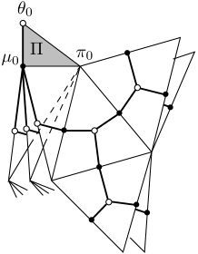
Figure 2. A portion of $\operatorname{{\mathcal{D}}}(H)/\operatorname{{\mathcal{G}}}$ and $\operatorname{{\mathcal{T}}}$ near the primitive orbits.

Through work of the first author [4], the action of $\operatorname{{\mathcal{G}}}$ on $\operatorname{{\mathcal{D}}}(H)$ is well-understood. A disk $D$ in $H$ is called primitive if there is a disk $E$ in $\overline{S^{3}-H}$ for which $\partial D$ and $\partial E$ intersect transversely in one point in $\partial H$. The primitive disks (regarded as vertices) span a contractible subcomplex $\operatorname{{\mathcal{P}}}(H)$ of $\operatorname{{\mathcal{D}}}(H)$, called the primitive subcomplex. The action of $\operatorname{{\mathcal{G}}}$ on $\operatorname{{\mathcal{P}}}(H)$ is as transitive as possible, indeed the quotient $\operatorname{{\mathcal{P}}}(H)/\operatorname{{\mathcal{G}}}$ is a single $2$-simplex $\Pi$ which is the image of any $2$-simplex of the first barycentric subdivision of $\operatorname{{\mathcal{P}}}(H)$. The vertices of $\Pi$ are $\pi_{0}$, the orbit of all primitive disks, $\mu_{0}$, the orbit of all pairs of disjoint primitive disks, and $\theta_{0}$, the orbit of all triples of disjoint primitive disks.

On the remainder of $\operatorname{{\mathcal{D}}}(H)$, the stabilizers of the action are as small as possible. A $2$-simplex which has two primitive vertices and one nonprimitive is identified with some other such simplices, then folded in half and attached to $\Pi$ along the edge $\langle\mu_{0},\pi_{0}\rangle$. The nonprimitive vertices of such $2$-simplices are exactly the disks in $\operatorname{{\mathcal{D}}}(H)$ that are disjoint from some primitive pair, and these are called simple disks. As tunnels, they are the upper and lower tunnels of $2$-bridge knots. The remaining $2$-simplices of $\operatorname{{\mathcal{D}}}(H)$ receive no self-identifications, and descend to portions of $\operatorname{{\mathcal{D}}}(H)/\operatorname{{\mathcal{G}}}$ that are treelike and are attached to one of the edges $\langle\pi_{0},\tau_{0}\rangle$ where $\tau_{0}$ is simple.

The tree $\widetilde{\operatorname{{\mathcal{T}}}}$ shown in Figure 1 is constructed as follows. Let $\operatorname{{\mathcal{D}}}^{\prime}(H)$ be the first barycentric subdivision of $\operatorname{{\mathcal{D}}}(H)$. Denote by $\widetilde{\operatorname{{\mathcal{T}}}}$ the subcomplex of $\operatorname{{\mathcal{D}}}^{\prime}(H)$ obtained by removing the open stars of the vertices of $\operatorname{{\mathcal{D}}}(H)$. It is a bipartite graph, with “white” vertices of valence $3$ represented by triples and “black” vertices of (countably) infinite valence represented by pairs. The valences reflect the fact that moving along an edge from a triple to a pair corresponds to removing one of its three disks, while moving from a pair to a triple corresponds to adding one of infinitely many possible third disks to a pair. The possible disjoint third disks that can be added are called the slope disks for the pair.

The image $\widetilde{\operatorname{{\mathcal{T}}}}/\operatorname{{\mathcal{G}}}$ of $\widetilde{\operatorname{{\mathcal{T}}}}$ in $\operatorname{{\mathcal{D}}}^{\prime}(H)/\operatorname{{\mathcal{G}}}$ is a tree $\operatorname{{\mathcal{T}}}$. The vertices of $\operatorname{{\mathcal{D}}}^{\prime}(H)/\operatorname{{\mathcal{G}}}$ that are images of vertices of $\operatorname{{\mathcal{D}}}(H)$ are not in $\operatorname{{\mathcal{T}}}$, but their links in $\operatorname{{\mathcal{D}}}^{\prime}(H)/\operatorname{{\mathcal{G}}}$ are subcomplexes of $\operatorname{{\mathcal{T}}}$. These links are known to be infinite trees. For each such vertex $\tau$ of $\operatorname{{\mathcal{D}}}^{\prime}(H)/\operatorname{{\mathcal{G}}}$, i. e. each tunnel, there is a unique shortest path in $\operatorname{{\mathcal{T}}}$ from $\theta_{0}$ to the vertex in the link of $\tau$ that is closest to $\theta_{0}$. This path is called the principal path of $\tau$, and this closest vertex is a triple, called the principal vertex of $\tau$. The two disks in the principal vertex, other than $\tau$, are called the principal pair of $\tau$. They are exactly the disks called $\mu^{+}$ and $\mu^{-}$ that play a key role in [17]. Figure 4 below shows the principal path of a certain tunnel.

The white vertices of $\operatorname{{\mathcal{T}}}$ correspond to unknotted $\theta$-curves in $S^{3}$, up to isotopy. For a white vertex gives a triple of nonseparating disks, dual to a $\theta$-curve in $H$ in which each arc crosses one of the disks and not the others. These are exactly the unknotted $\theta$-curves, in that a regular neighborhood is isotopic to $H$ which is part of a Heegaard splitting of $S^{3}$. Two such $\theta$-curves in $H$ are isotopic in $S^{3}$ exactly when they are equivalent under the Goeritz group, so the white vertices of $\operatorname{{\mathcal{T}}}$ give the isotopy classification.

2. The cabling construction and the binary invariants

In a sentence, the cabling construction is to “Think of the union of $K$ and the tunnel arc as a $\theta$-curve, and rationally tangle the ends of the tunnel arc and one of the arcs of $K$ in a neighborhood of the other arc of $K$.” We sometimes call this “swap and tangle,” since one of the arcs in the knot is exchanged for the tunnel arc, then the ends of other arc of the knot and the tunnel arc are connected by a rational tangle. Figure 3 illustrates two cabling constructions, one starting with the trivial knot and obtaining the trefoil, then another starting with the tunnel of the trefoil.

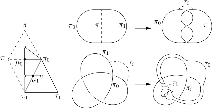
Figure 3. Examples of the cabling construction.

More precisely, begin with a triple $\{\lambda,\rho,\tau\}$, where $\{\lambda,\rho\}$ is the principal pair of $\tau$. Choose one of the disks of $\{\lambda,\rho\}$, say $\rho$, and a slope disk $\tau^{\prime}$ of the pair $\{\rho,\tau\}$, other than $\lambda$. This is a cabling operation producing the tunnel $\tau^{\prime}$ from $\tau$. The principal vertex of $\tau^{\prime}$ is $\{\rho,\tau,\tau^{\prime}\}$.

Unless otherwise stated, the slope disk $\tau^{\prime}$ is chosen to be nonseparating in $H$. A cabling operation using a separating disk as $\tau^{\prime}$ produces a tunnel number $1$ link, and the cabling process cannot be continued. This case will be discussed in Section 9.

Theorem 13.2 of [5] shows that every tunnel of every tunnel number $1$ knot can be obtained by a uniquely determined sequence of cabling constructions. A tunnel $\tau_{0}$ produced from the tunnel of the trivial knot by a single cabling construction is called a simple tunnel. As already noted, these are the “upper and lower” tunnels of $2$-bridge knots. A tunnel is called semisimple if it is disjoint from a primitive disk, but not from any primitive pair.

A $(1,1)$-knot is a knot that can be put into $1$-bridge position with respect to a Heegaard torus of $S^{3}$. Let $K$ be a $(1,1)$-knot, whose Heegaard torus splits $S^{3}$ into two solid tori $V$ and $W$. Associated to this $(1,1)$-position are two tunnels obtained as follows. Let $\alpha_{V}$ be an arc in $V$ with endpoints in $K$, such that the union of $\alpha_{V}$ with the arc in $K\cap V$ bounded by the endpoints of $\alpha_{V}$ is a core circle of $V$. Then $\alpha_{V}$ determines a tunnel of $K$; the corresponding tunnel constructed in $W$ is the other one. Tunnels arising in this way are called $(1,1)$-tunnels, and are exactly the simple and semisimple tunnels.

A tunnel is called regular if it is not primitive, simple, or semisimple.

There is a procedure for assigning rational slopes which record the rational tangle used in a cabling construction. We will not need these slopes in our study of depth, although we will include them, in an inessential way, in our discussion of the torus knot examples in Section 8, and they also appear briefly in Remark 6.4. The slope invariants are usually not needed for working with depth because the depth is completely determined by the second set of invariants associated to a tunnel, the “binary” invariants $s_{2},s_{3},\ldots\,$, $s_{n}$, which we now define.

We have already mentioned that for every tunnel $\tau$, there is a unique sequence of tunnels $\tau_{0},\ldots\,$, $\tau_{n}=\tau$ such that $\tau_{0}$ is simple and for each $i\geq 1$, $\tau_{i}$ is obtained from $\tau_{i-1}$ by a cabling construction. The cabling that produces $\tau_{i}$ retains one arc of the associated knot $K_{\tau_{i-1}}$ of $\tau_{i-1}$, and replaces the other with a tangle, producing $K_{\tau_{i}}$. The invariant $s_{i}$ is $1$ exactly when this cabling replaces the arc that was retained by the previous cabling, otherwise $s_{i}$ is $0$.

A tunnel is simple or semisimple if and only if all $s_{i}=0$. The reason is that both conditions characterize cabling sequences in which one of the original primitive disks is retained in every cabling; this corresponds to the fact that the union of the tunnel arc and one of the arcs of the knot is unknotted.

There are two formal definitions of the binary invariants. The first is in terms of the principal path $\theta_{0}$, $\mu_{0}$, $\mu_{0}\cup\{\tau_{0}\}$, $\mu_{1},\ldots\,$, $\mu_{n}$, $\mu_{n}\cup\{\tau_{n}\}$, where the $\mu_{i}$ are the “black” vertices, the $\mu_{i}\cup\{\tau_{i}\}$ are the “white” vertices, and $\tau=\tau_{n}$: $s_{i}=0$ or $s_{i}=1$ according to whether or not the unique disk of $\mu_{i}\cap\mu_{i-1}$ equals the unique disk of $\mu_{i-1}\cap\mu_{i-2}$. Equivalently, each cabling operation begins with a triple of disks $\{\lambda_{i-1},\rho_{i-1},\tau_{i-1}\}$ and finishes with $\{\lambda_{i},\rho_{i},\tau_{i}\}$. For $i\geq 2$, put $s_{i}=1$ if $\{\lambda_{i},\rho_{i},\tau_{i}\}=\{\tau_{i-2},\tau_{i-1},\tau_{i}\}$, and $s_{i}=0$ otherwise. Figure 4 shows the principal path of a tunnel with binary invariants $0011100011100$.

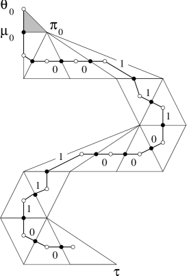
Figure 4. The principal path of a tunnel $\tau$ having binary invariants $0011100011100$, or equivalently with step sequence “DRRRDRDLLLDLDRR”.

From the viewpoint of a traveler along the principal path, $s_{i}=1$ means a change from making right turns (at the white vertices) to left turns, or from left turns to right, while $s_{i}=0$ means a turn in the same direction as the previous turn. Let us say that a step of the principal path is a portion between successive white vertices. A principal path can then be described as a step sequence. This is a string of symbols “L”, “R”, or “D”, for “left”, “right”, and “down” as seen from the reader’s viewpoint (as opposed to the “left” and “right” of a traveler along the path). For the example of Figure 4, the step sequence is “DRRRDRDLLLDLDRR”. In general, the initial step of a principal path is always “D”, and the second step, due to the standard way that we draw the picture, is “R”. Each subsequent step corresponds to a binary invariant. An “L” can only be followed by another “L” or a “D”, according as the corresponding binary invariant $s$ is $0$ or $1$, and similarly an “R” is followed by another “R” or a “D”, according as $s$ is $0$ or $1$. When the previous step is “D”, the effect of $s$ depends on the step before one that produces the “D”. If the “D” is in a sequence “LD”, then the next step is “R” or “L” according as $s$ is $0$ or $1$, while if it is in “RD”, then the next step is “L” or “R” according as $s$ is $0$ or $1$.

Functions that translate between the binary sequence and step sequence descriptions are included in the software at [8]. The main functions there accept either form of input for principal paths.

3. Distance and depth

The (Hempel) distance $\operatorname{dist}(\tau)$ is the shortest distance in the curve complex of $\partial H$ from $\partial\tau$ to a loop that bounds a disk in $\overline{S^{3}-H}$ (see J. Johnson [11] and Y. Minsky, Y. Moriah, and S. Schleimer [13]). It is well-defined since the action of the Goeritz group on $\partial H$ preserves the set of loops that bound disks in $H$ and the set that bound in $\overline{S^{3}-H}$.

A nonseparating disk has distance $1$ if and only if it is primitive, since both conditions are equivalent to the condition that cutting $H$ along the disk produces an unknotted solid torus. Therefore the tunnel of the trivial knot is the only tunnel of distance $1$. A simple or semisimple tunnel has distance $2$, since it is disjoint from a primitive disk. There are, however, regular tunnels of distance $2$. It is an easy observation that the “middle” tunnels of torus knots all have distance $2$, and in most cases these are regular.

When $\Sigma_{\tau}=(\overline{H-\operatorname{Nbd}(K_{\tau})},\overline{S^{3}-H})$ is a Heegaard splitting of the complement of $K_{\tau}$, the (Hempel) distance $\operatorname{dist}(\Sigma_{\tau})$ is the minimal distance in the curve complex of $\partial H$ between the boundary of a disk in $\overline{H-\operatorname{Nbd}(K_{\tau})}$ and the boundary of a disk in $\overline{S^{3}-H}$ (where the disks may be separating). Clearly, $\operatorname{dist}(\Sigma_{\tau})\leq\operatorname{dist}(\tau)$. On the other hand, Johnson [11, Lemma 11] proved that

Lemma 3.1 (Johnson).

$\operatorname{dist}(\tau)\leq\operatorname{dist}(\Sigma_{\tau})+1$.

M. Scharlemann and M. Tomova [18] proved the following stability result:

Theorem 3.2 (Scharlemann-Tomova).

Genus-$g$ Heegaard splittings of distance more than $2g$ are isotopic.

Using Lemma 3.1 and Theorem 3.2, Johnson [11, Corollary 13] deduced the following:

Theorem 3.3 (Johnson).

If $\tau$ is a tunnel of a tunnel number $1$ knot $K_{\tau}$ and $\operatorname{dist}(\tau)>5$, then $\tau$ is the unique tunnel of $K_{\tau}$.

Theorem 15.2 of [5] determines all orientation-reversing self-equivalences of tunnels:

Theorem 3.4.

Let $\tau$ be a tunnel of a tunnel number $1$ knot or link. Suppose that $\tau$ is equivalent to itself by an orientation-reversing equivalence. Then $\tau$ is the tunnel of the trivial knot, the trivial link, or the Hopf link.

Combining Theorems 3.3 and 3.4 gives the following:

Corollary 3.5.

If $\tau$ is a tunnel of a tunnel number $1$ knot, and $\operatorname{dist}(\tau)>5$, then $K_{\tau}$ is not amphichiral.

For Theorem 3.4 shows that an orientation-reversing equivalence from $K_{\tau}$ to $K_{\tau}$ would produce a second tunnel for $K_{\tau}$.

Distance also has implications for hyperbolicity:

Theorem 3.6.

If $K_{\tau}$ is a torus knot or a satellite knot, then $\operatorname{dist}(\tau)\leq 2$. Consequently, if $\operatorname{dist}(\tau)\geq 3$, then $K_{\tau}$ is hyperbolic.

Proof.

We have already mentioned the fact [6] that the middle tunnels of torus knots have distance $2$. The other tunnels of torus knots are simple or semisimple, so also have distance $2$. K. Morimoto and M. Sakuma [15] found all tunnels of tunnel number $1$ satellite knots, showing in particular that they are semisimple. ∎

The depth of $\tau$ is the simplicial distance $0pt(\tau)$ in the $1$-skeleton of $\operatorname{{\mathcal{D}}}(H)/\operatorname{{\mathcal{G}}}$ from $\tau$ to the primitive vertex $\pi_{0}$. From the definitions, $\tau$ is primitive if and only if $0pt(\tau)=0$, is simple or semisimple if and only if $0pt(\tau)=1$, and is regular if and only if $0pt(\tau)\geq 2$.

The inequality

$$\operatorname{dist}(\tau)-1\leq 0pt(\tau)$$

mentioned in the introduction is immediate from the definitions. On the other hand, we have already noted that the middle tunnels of torus knots have distance $2$, but we will see in Section 8 that their depths can be arbitrarily large.

In terms of the step sequence describing the principal path of a tunnel, the depth is simply the number of D’s that appear. One can, of course, determine the depth directly from the binary invariants. A maximal block of $1$’s in the binary word $s_{2}\cdots s_{n}$ has the following effect: its first, third, fifth, and so on terms will produce a downward step, increasing the depth, while the other terms correspond to horizontal steps, keeping the same depth. This gives the following simple algorithm to compute $0pt(\tau)$ from the binary invariants of $\tau$:

1. Write the binary word $s_{2}s_{3}\cdots s_{n}$ as $O_{1}Z_{1}O_{2}Z_{2}\cdots O_{k}Z_{k}$, where $O_{i}$ and $Z_{i}$ are respectively maximal blocks of ones and zeros (thus $O_{1}$ and $Z_{k}$ may have length $0$, while all others have positive length).

2. The depth of $\tau$ is $1+\displaystyle\sum_{j=1}^{k}\lceil\operatorname{length}(O_{i})/2\rceil$, where $\lceil\operatorname{length}(O_{i})/2\rceil$ denotes the least integer greater than or equal to $\operatorname{length}(O_{i})/2$.

4. Tunnel leveling

Roughly speaking, the Tunnel Leveling Theorem of Goda, Scharlemann, and Thompson says that a tunnel arc of a tunnel number one knot can be slid so that it lies in a level sphere of some minimal bridge position of the knot. Here is the rather technical version of the Tunnel Leveling Theorem that we will need. Illustrations of conclusions (i) and (ii) of the theorem appear in the first drawings of Figure 5 and Figure 6 respectively.

Theorem 4.1 (Goda-Scharlemann-Thompson).

Let $\{\lambda,\rho\}$ be the principal pair of a tunnel $\tau$, and let $\theta$ be the $\theta$-curve associated to the principal vertex $\{\lambda,\rho,\tau\}$ of $\tau$. Write $T$ for the arc dual to $\tau$, and $L$ and $R$ for the other two arcs of $\theta$ that are dual to $\lambda$ and $\rho$, so that $K_{\tau}=L\cup R$, $K_{\lambda}=R\cup T$, and $K_{\rho}=L\cup T$. Then there is a minimal bridge position of $K_{\tau}$ for which either:

1. $T$ is slid to an arc in a level sphere, and $T$ connects two bridges of $K_{\tau}$. Moreover, $K_{\tau}\cup T$ is isotopic to the original $\theta$. Or,

2. $T$ is slid to an eyeglass in a level sphere. The endpoints of $T$ can be slid slightly apart, moving $T$ out of the level sphere, producing $K_{\tau}\cup T$ isotopic to the original $\theta$, and showing that one of $K_{\lambda}$ or $K_{\rho}$ is a trivial knot, and consequently $\tau$ is simple or semisimple.

and furthermore, in the $n$-strand trivial tangle above the level sphere:

1. In case (i), the arcs are parallel to a collection of disjoint arcs in the level sphere, which meet $T$ only in its endpoints.

2. In case (ii), the $n-1$ arcs not meeting $T$ are parallel to a collection of disjoint arcs in the level sphere, each meeting the eyeglass in a single point.

Proof.

By Theorem 1.8 of [10], we may move $K_{\tau}\cup T$, possibly using slide moves of $T$ as well as isotopy, so that $K_{\tau}$ is in minimal bridge position and $T$ either lies on a level sphere and connects two bridges of $K_{\tau}$, or $T$ is slid to an “eyeglass”. Since the leveling process involves sliding the tunnel arc $T$, there is a priori no reason for the resulting $\theta$-curve to be isotopic to the original $\theta$. But Corollary 3.4 and Theorem 3.5 (combined with Lemma 2.9) of [17] show that in (i) and (ii), the dual disks to the other two arcs of the $\theta$-curve are the disks called $\mu^{+}$ and $\mu^{-}$ there. By Lemma 14.1 of [5], these disks are the principal pair of $\tau$, that is, $\lambda$ and $\rho$. Therefore the resulting $\theta$-curve is isotopic to the original $\theta$. Finally, the description of the trivial tangle above the level sphere in (iii) is from Theorem 6.1 of [10], and in (iv) from Corollary 6.2 of [10], which relies on [9]. ∎

A tunnel arc $T$ satisfying conclusion (i) of the Tunnel Leveling Theorem is said to be in level arc position, while for conclusion (ii), after sliding the endpoints apart to produce $\theta$, it is in eyeglass position. If it is in one of these two positions, it may be said to be in level position.

A tunnel arc satisfying all the requirements of level position except that the number of bridges of $K_{\tau}$ is not necessarily minimal is said to be in weak level position. The number of bridges is then called the bridge count, denoted $\operatorname{bc}(K_{\tau})$ and dependent, of course, on the choice of weak level position.

Suppose that $\tau$ is in weak level arc position. The endpoints of $\tau$ cut $K_{\tau}$ into two arcs, one dual to $\lambda$ and the other dual to $\tau$. By a simple isotopy, we may assume that one end of the arc dual to $\lambda$ leaves the endpoints of the tunnel arc in the upward direction, and the other leaves in the downward direction. For if both leave in the same direction, we can slide an endpoint of the tunnel arc over one of the arches, achieving a level position for which the two ends leave in different directions. We then call this an admissible weak level arc position.

When $\tau$ is in weak level arc position, each of the local maxima of $K_{\tau}$ lies in exactly one of $K_{\lambda}$ or $K_{\rho}$. The numbers that lie in each are called the relative bridge counts of $K_{\lambda}$ and $K_{\rho}$ for the weak level arc position of $\tau$, and denoted by $\operatorname{rbc}(K_{\lambda})$ and $\operatorname{rbc}(K_{\rho})$. Clearly $\operatorname{bc}(K_{\tau})=\operatorname{rbc}(K_{\lambda})+\operatorname{rbc}(K_{\rho})$. If $\tau$ is in weak eyeglass position, with $K_{\lambda}$ a trivial knot, then we define $\operatorname{rbc}(K_{\lambda})=1$ and $\operatorname{rbc}(K_{\rho})=\operatorname{bc}(K_{\tau})$. One always has $\operatorname{br}(K_{\gamma})\leq\operatorname{rbc}(K_{\gamma})$.

A first consequence of Theorem 4.1 is the following.

Lemma 4.2.

Let $\tau$ be a tunnel of a nontrivial knot, and let $\{\lambda,\rho\}$ be the principal pair of $\tau$. Then $\operatorname{br}(K_{\lambda})+\operatorname{br}(K_{\rho})-1\leq\operatorname{br}(K_{\tau})$. If $\tau$ is regular, then $\operatorname{br}(K_{\lambda})+\operatorname{br}(K_{\rho})\leq\operatorname{br}(K_{\tau})$.

Proof.

Apply Theorem 4.1 to $\tau$. If the tunnel arc is in level arc position, which may be assumed to be admissible, then we have $\operatorname{br}(K_{\lambda})+\operatorname{br}(K_{\tau})\leq\operatorname{rbc}(K_{\lambda})+\operatorname{rbc}(K_{\tau})=\operatorname{br}(K_{\tau})$. If the tunnel arc is in eyeglass position, producing, say, $K_{\lambda}$ trivial, then we have $\operatorname{br}(K_{\lambda})+\operatorname{br}(K_{\rho})\leq 1+\operatorname{rbc}(K_{\rho})=1+\operatorname{br}(K_{\tau})$, giving the inequality. If $\tau$ is regular, then the eyeglass configuration cannot occur, giving the stronger inequality. ∎

5. Efficient cabling and the Tunnel Leveling Addendum

In this section, we will prove the following theorem:

Theorem 5.1 (Tunnel Leveling Addendum).

Let $\tau$ be a tunnel with principal vertex $\{\lambda,\rho,\tau\}$. If $\tau$ is not simple, choose notation so that $\rho$ is the tunnel directly preceding $\tau$ in the cabling sequence for $\tau$. Assume that $\tau$ is not the tunnel of the trivial knot or a simple tunnel of a $(2n+1,2)$ torus knot. Then either

1. All level positions of $\tau$ are level arc positions, and $\operatorname{br}(K_{\tau})=\operatorname{br}(K_{\rho})+\operatorname{br}(K_{\lambda})$, or

2. All level positions of $\tau$ are eyeglass positions, $\tau$ is semismiple, and $\operatorname{br}(K_{\tau})=\operatorname{br}(K_{\rho})$.

The exceptional case of the Tunnel Leveling Addendum is detailed in the next theorem, which is simply a restatement of some results from the work of K. Morimoto and M. Sakuma on tunnels of $2$-bridge knots [15]:

Theorem 5.2.

The trefoil knots have unique tunnels, which are simple and can be put into either level arc position or eyeglass position. For the other $(2n+1,2)$ torus knots, there are two simple tunnels, of which one can be put into both kinds of level position, and the other only into level arc position.

Of course the trivial knot has a unique tunnel, which can only be leveled in eyeglass position.

It is important to understand the geometric content of the Tunnel Leveling Addendum from the viewpoint of the Tunnel Leveling Theorem 4.1. Apart from the exceptional cases, the Addendum says that when a tunnel $\tau$ is leveled, giving a positioning of the $\theta$-curve associated to the principal vertex $\{\lambda,\rho,\tau\}$ of $\tau$, then (possibly after trivial repositioning) the copies of $K_{\lambda}$ and $K_{\rho}$ in that $\theta$-curve are in minimal bridge position.

In this section we will prove the Tunnel Leveling Addendum and Theorem 5.2, and in preparation for this we now introduce the technique of efficient cabling. The basic construction is shown in Figure 5, whre notation is selected so that the cabling will replace $\lambda$ and retain $\rho$. We start with $\tau$ in admissible weak level arc position, as shown in the left-hand drawing. There may, of course, be many more bridges, some in $K_{\rho}$ and some in $K_{\lambda}$. A cabling of some arbitrary slope replaces $\lambda$ with a new tunnel $\tau^{\prime}$; the rational tangle in $K_{\tau^{\prime}}$ created by the cabling is inside a ball represented by the circle in the middle drawing. We may then reposition $K_{\tau^{\prime}}$ as in the right-hand drawing of Figure 5, by “moving the ball up to engulf infinity,” in such a way that the rectangle in the drawing contains a $4$-strand braid. The arc dual to $\tau^{\prime}$ is in weak level arc position, and by a further isotopy, if necessary, we may assume that it is in admissible weak level arc position.

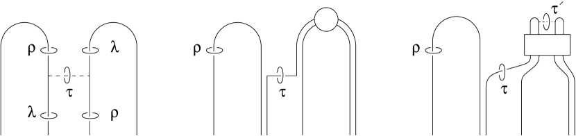
Figure 5. Efficient cabling from admissible weak level arc position.

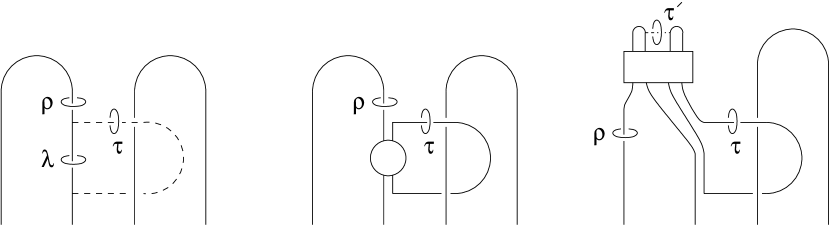
Figure 6. Efficient cabling from eyeglass position, producing a semisimple tunnel.

The corresponding construction for a tunnel in weak eyeglass position can produce either another semisimple tunnel or a regular tunnel. The resulting tunnel is in weak level arc position, which by isotopy is also assumed to be admissible. Efficient cablings for each of the two possibilities are shown in Figures 6 and 7, and the constructions should be clear from the discussion of the weak level arc case.

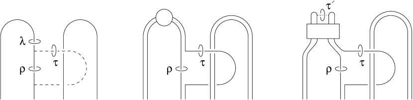
Figure 7. Efficient cabling from eyeglass position, producing a regular tunnel.

The next result details the effect of efficient cabling on bridge counts. The notations $K$ and $K^{\prime}$ are used to indicate knots obtained from the $\theta$-curves associated to $\{\lambda,\rho,\tau\}$ and $\{\rho,\tau,\tau^{\prime}\}$ respectively:

Proposition 5.3.

Suppose that $\tau$ is in weak level arc or weak eyeglass position, and that a cabling operation as in Figure 5, 6, or 7 is performed, producing a new tunnel $\tau^{\prime}$ with principal vertex $\{\rho,\tau,\tau^{\prime}\}$, and producing a tunnel arc $T^{\prime}$ for which $\tau^{\prime}$ is in level arc position. Then

1. $\operatorname{rbc}(K_{\rho}^{\prime})=\operatorname{rbc}(K_{\rho})$.

2. $\operatorname{rbc}(K_{\tau}^{\prime})=\operatorname{bc}(K_{\tau})$.

3. $\operatorname{bc}(K_{\tau^{\prime}}^{\prime})=\operatorname{bc}(K_{\tau})+\operatorname{rbc}(K_{\rho})$.

Proof.

The third equality follows from the first two. The first two are seen by examination of Figures 5, 6, and 7. For example, let us consider Figure 5. In the leftmost drawing, denote the arcs dual to $\lambda$, $\rho$, and $\tau$ by $L$, $R$, and $T$ respectively. In the rightmost drawing, after the cabling producing $K_{\tau^{\prime}}^{\prime}$ has been performed, denote the dual arcs by $R_{1}$, $T_{1}$, and $T_{1}^{\prime}$, where the latter is horizontal. By isotopy we may assume that $\tau^{\prime}$ is also in admissible weak level arc position. The number of bridges that we see in $R_{1}\cup T_{1}^{\prime}$ equals the number that appeared in $R$ plus the number that appeared in $L$, showing that $\operatorname{rbc}(K_{\tau}^{\prime})=\operatorname{bc}(K_{\tau})$. The number of bridges in $T_{1}\cup T_{1}^{\prime}$ is the number that appeared in $L$, so $\operatorname{rbc}(K_{\rho}^{\prime})=\operatorname{rbc}(K_{\rho})$. The arguments for Figures 6 and 7 are similar. ∎

We are now ready to prove the Tunnel Leveling Addendum and Theorem 5.2 simultaneously. The tunnel called $\tau$ in the statement of the Addendum will be denoted by $\tau^{\prime}$ in our argument. Its principal vertex will be written as $\{\rho,\tau,\tau^{\prime}\}$. If $\tau^{\prime}$ is not simple, then we assume that $\tau$ is the tunnel that precedes $\tau^{\prime}$ in the cabling sequence of $\tau^{\prime}$, and the principal vertex of $\tau$ will be written as $\{\lambda,\rho,\tau\}$. As in Proposition 5.3, we use $K$ and $K^{\prime}$ to indicate knots obtained from the $\theta$-curves associated to $\{\lambda,\rho,\tau\}$ and $\{\rho,\tau,\tau^{\prime}\}$ respectively. Note, however, that $K_{\rho}$ and $K_{\tau}$ are equivalent to $K^{\prime}_{\rho}$ and $K^{\prime}_{\tau}$ and hence $\operatorname{br}(K^{\prime}_{\rho})=\operatorname{br}(K_{\rho})$ and $\operatorname{br}(K^{\prime}_{\tau})=\operatorname{br}(K_{\tau})$.

We will induct on the length of the cabling sequence of $\tau^{\prime}$. If the length is $1$, then $\tau^{\prime}$ is an upper or lower tunnel of the $2$-bridge knot $K^{\prime}_{\tau^{\prime}}$, so can be put into level arc position. Each of $K^{\prime}_{\tau}$ and $K^{\prime}_{\rho}$ is a trivial knot so has bridge number $1$. Therefore we have $\operatorname{br}(K^{\prime}_{\tau^{\prime}})=\operatorname{br}(K^{\prime}_{\rho})+\operatorname{br}(K^{\prime}_{\tau})$. So conclusion (a) of the Tunnel Leveling Addendum holds for $\tau^{\prime}$, provided that $\tau^{\prime}$ cannot also be put into eyeglass position.

The homeomorphism classfication of tunnels of $2$-bridge knots is given in Table 5.2(B) of [15], and only in the cases called $2$, $3$, and $6$ there does there exist a simple tunnel which can also be put into eyeglass position. Those cases are defined in Lemma 5.1 of [15], and upon examination are found to be exactly the $2$-bridge torus knots. Since this is the excluded case in the Tunnel Leveling Addendum, the Addendum holds for tunnels whose cabling sequences have length $1$. Closer examination of the tunnel classification in [15] verifies the precise statement in Theorem 5.2, whose proof is now complete.

Assume now that the length of the cabling sequence of $\tau^{\prime}$ is greater than $1$. Put $\tau$ in level position and obtain $\tau^{\prime}$ by efficient cabling as in one of Figures 5, 6, or 7.

Suppose first that the resulting weak level arc position for $\tau^{\prime}$ is actually a level arc position. Using Proposition 5.3 and induction, we have $\operatorname{br}(K^{\prime}_{\tau^{\prime}})=\operatorname{rbc}(K^{\prime}_{\tau})+\operatorname{rbc}(K^{\prime}_{\rho})=\operatorname{bc}(K_{\tau})+\operatorname{rbc}(K_{\rho})=\operatorname{br}(K_{\tau})+\operatorname{br}(K_{\rho})$.

Suppose now that the weak level arc position for $\tau^{\prime}$ is not level arc position. Then $\operatorname{br}(K^{\prime}_{\tau^{\prime}})<\operatorname{bc}(K^{\prime}_{\tau^{\prime}})=\operatorname{rbc}(K^{\prime}_{\tau})+\operatorname{rbc}(K^{\prime}_{\rho})=\operatorname{bc}(K_{\tau})+\operatorname{rbc}(K_{\rho})=\operatorname{br}(K_{\tau})+\operatorname{br}(K_{\rho})$, so Lemma 4.2 tells us that $\tau^{\prime}$ is semisimple and $\operatorname{br}(K_{\tau^{\prime}}^{\prime})=\operatorname{br}(K_{\tau})+\operatorname{br}(K_{\rho})-1$. But $\rho$ is primitive, since the principal vertex of every semismiple tunnel contains a primitive disk, and $\tau$ is not primitive since $\tau^{\prime}$ is not simple. Therefore $\operatorname{br}(K_{\rho})=1$ and $\operatorname{br}(K_{\tau})=\operatorname{br}(K^{\prime}_{\tau^{\prime}})$.

In the latter case, $\tau^{\prime}$ cannot be put into level arc position, since then we would have $\operatorname{br}(K^{\prime}_{\tau^{\prime}})=\operatorname{rbc}(K^{\prime}_{\tau})+\operatorname{rbc}(K^{\prime}_{\rho})\geq\operatorname{br}(K^{\prime}_{\tau})+\operatorname{br}(K^{\prime}_{\rho})>\operatorname{br}(K_{\tau})$. So either all level positions are level arc positions, or all are eyeglass positions. This completes the proof of the Tunnel Leveling Addendum and Theorem 5.2.

The next two corollaries are convenient restatements of parts of the Tunnel Leveling Addendum.

Corollary 5.4.

Let $\tau$ be a regular tunnel with principal vertex $\{\lambda,\rho,\tau\}$. Then $\operatorname{br}(K_{\rho})+\operatorname{br}(K_{\lambda})=\operatorname{br}(K_{\tau})$.

Corollary 5.5.

Let $\tau$ be a semisimple tunnel with principal vertex $\{\pi_{0},\rho,\tau\}$. Then $\operatorname{br}(K_{\rho})=\operatorname{br}(K_{\tau})$ or $\operatorname{br}(K_{\tau})=\operatorname{br}(K_{\rho})+1$, according to whether all level positions for $\tau$ are eyeglass positions or all are level arc positions.

6. Fibonacci functions

Let $\tau$ be a tunnel and write the cabling sequence of $\tau$ as $\tau_{0}$, $\tau_{1}\,\ldots$, $\tau_{m-1}$, $\tau_{m},\ldots\,$, $\tau_{n-1}=\tau$, where $\tau_{i}$ is simple or semisimple exactly when $i\leq m-1$. That is, $\tau$ is produced by $n$ cablings, the first $m$ of which produce depth-$1$ tunnels. In particular, $n=m$ when $0pt(\tau)=1$.

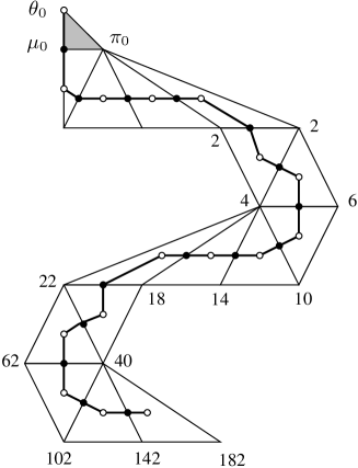
Figure 8.

The principal vertex of $\tau_{0}$ has the form $\{\pi_{0},\pi_{1},\tau_{0}\}$, where $\pi_{0}$ and $\pi_{1}$ are primitive. If we put $\tau_{-1}=\pi_{0}$, the trivial tunnel, then for each $k\geq 1$, the principal vertex of $\tau_{k}$ is of the form $\{\tau_{i},\tau_{k-1},\tau_{k}\}$ for some $i$. If $n>m$, that is, if $\tau$ is regular, then the first tunnel of depth $2$ is $\tau_{m}$, and its principal vertex is $\{\tau_{m-2},\tau_{m-1},\tau_{m}\}$. We then define the Fibonacci function $F_{\tau}$ of a regular tunnel $\tau$ as follows. To compute $F_{\tau}(a,b)$, put $b_{m-2}=a$, $b_{m-1}=b$, and for $m\leq k\leq n-1$, put $b_{k}=b_{i}+b_{k-1}$, where $\{\tau_{i},\tau_{k-1},\tau_{k}\}$ is the principal vertex of $\tau_{k}$. Then, put $F_{\tau}(a,b)=b_{n-1}$. Figure 8 shows how to calculate that $F_{\tau}(2,2)=182$ for a certain depth-$5$ tunnel with $m=4$ and $n=15$.

Theorem 6.1.

Let $\tau$ be a simple or semisimple tunnel produced by $m$ cablings. Then $2\leq\operatorname{br}(K_{\tau})\leq m+1$.

Proof.

Induct on $m$, using Corollary 5.5. ∎

Theorem 6.2.

Let $\tau$ be a regular tunnel whose cabling sequence contains $m$ tunnels of depth $1$. Let $b_{i}=\operatorname{br}(K_{\tau_{i}})$ for $i\in\{m-2,m-1\}$. Then $\operatorname{br}(K_{\tau})=F_{\tau}(b_{m-2},b_{m-1})$.

Proof.

Induct on the length of the cabling sequence of $\tau$, using Corollary 5.4. ∎

Theorem 6.3 (Bridge Number Set).

Suppose that a knot $K$ has a tunnel $\tau$ produced by $n\geq 2$ cabling operations, of which the first $m$ produce simple or semisimple tunnels. Then $\operatorname{br}(K)$ is one of the $2m-2$ values $F_{\tau}(a,b)$ for $2\leq a\leq b\leq a+1\leq m+1$.

Proof.

By Theorem 6.1, we have $2\leq\operatorname{br}(K_{\tau_{m-2}})\leq m$, and by Corollary 5.5, $\operatorname{br}(K_{\tau_{m-2}})\leq\operatorname{br}(K_{\tau_{m-1}})\leq\operatorname{br}(K_{\tau_{m-2}})+1$. The result now follows from Theorem 6.2. ∎

Remark 6.4.

We believe that for every principal path, each of the $2m-2$ possible values given in the Bridge Number Set Theorem occurs as a bridge number for some knots having a tunnel constructed using the given principal path. This is clear for $m=2$. In that case, the cabling sequence has only two tunnels $\tau_{0}$ and $\tau_{1}$ of depth $1$. When $\tau_{1}$ is a semisimple tunnel of a $2$-bridge knot, $\operatorname{br}(K_{\tau_{0}})=\operatorname{br}(K_{\tau_{1}})=2$, and there are many examples where $\operatorname{br}(K_{\tau_{0}})=2$ and $\operatorname{br}(K_{\tau_{1}})=3$, such as semisimple tunnels of torus knots [6]. So choosing cabling sequences that start with these two types of examples gives tunnels whose knots have bridge numbers $F_{\tau}(2,2)$ and $F_{\tau}(2,3)$.

For $m=3$, we need to produce the sequences $(2,2,2)$, $(2,2,3)$, $(2,3,3)$, and $(2,3,4)$ for $(\operatorname{br}(K_{\tau_{0}}),\operatorname{br}(K_{\tau_{1}}),\operatorname{br}(K_{\tau_{2}}))$. Semisimple tunnels of $2$-bridge knots give $(2,2,2)$. For $(2,2,3)$, we choose $\tau_{1}$ to be a semisimple tunnel of a $2$-bridge knot and choose any cabling with slope not of the form $\pm 2+1/k$ to produce $\tau_{2}$; the results of [5, Section 15] then show that $K_{\tau_{2}}$ cannot be $2$-bridge. By Corollary 5.5, $\operatorname{br}(K_{\tau_{2}})=3$. For $(2,3,3)$, we start by constructing $\tau_{1}$ to be an upper tunnel of a $3$-bridge torus knot, say the $(4,3)$ torus knot, as explained in [6]. The tunnel arc shown in [6] can be put into eyeglass level position with $K_{\tau_{1}}$ having three bridges, then a cabling which is geometrically like those of Figure 14 of [5] does not raise bridge number, so $\operatorname{br}(K_{\tau_{2}})=3$ as well. Finally, for $(2,3,4)$ we can just use the upper tunnel of the $(5,4)$ torus knot, obtained by three cablings as in [6].

For larger $m$, from upper tunnels of torus knots we obtain the bridge number sequence $(2,3,4,\ldots,m+1)$, and hence realize $F_{\tau}(m,m+1)$. And the idea for $(2,2,3)$ extends to realized $(2,2,\ldots,2,3)$, so $F_{\tau}(2,3)$ occurs as a bridge number. If we start with such an upper tunnel sequence, for which the upper tunnel is in eyeglass position, and then at some point begin using cablings as in Figure 14 of [5], we obtain all sequences of the form $(2,3,4,\ldots,k-1,k,k,\ldots,k)$, giving the $m-1$ values $F_{\tau}(k,k)$. So at least these $m+1$ values in the bridge number set are known to occur. If we follow the latter procedure, but use a complicated tangle for the final cabling, then the sequences $(2,3,4,\ldots,k-1,k,k,\ldots,k,k+1)$ should also be obtained, giving the remaining $m-3$ values $F_{\tau}(k,k+1)$ for $3\leq k\leq m-1$. Unfortunately we lack a means to prove that the final knot has bridge number $k+1$ rather than $k$.

A peculiar consequence of Theorem 6.2 is the following:

Corollary 6.5.

Let $\tau$ be a regular tunnel and let $\tau_{m}$ be the first tunnel of depth $2$ in the cabling sequence of $\tau$. Then $\operatorname{br}(K_{\tau})$ is completely determined by the principal path of $\tau$ and the value of $\operatorname{br}(K_{\tau_{m}})$. In fact,

$$\operatorname{br}(K_{\tau})=F_{\tau}([\operatorname{br}(K_{\tau_{m}})/2],[(\operatorname{br}(K_{\tau_{m}})+1)/2])\ .$$

Proof.

By Corollary 5.4, $\operatorname{br}(K_{\tau_{m-2}})+\operatorname{br}(K_{\tau_{m-1}})=\operatorname{br}(K_{\tau_{m}})$. Since also $\operatorname{br}(K_{\tau_{m-2}})$ and $\operatorname{br}(K_{\tau_{m-1}})$ differ by at most $1$, their values must be as in the statement of the corollary. ∎

It is not difficult to implement Theorems 6.2 and 6.3 computationally [8]:

Depth> fibonacci( ’0011100011100’, 2, 2, verbose=True )

F $\backslash$tau( 2, 2 ) = 182

The iteration sequence is:

2, 2, 4, 6, 10, 14, 18, 22, 40, 62, 102, 142, 182

Depth> bridgeSet( ’0011100011100’ )

[182, 232, 273, 323, 364, 414]

7. Bounding bridge number

Using the results of Section 6, we can give some general bounds on bridge number.

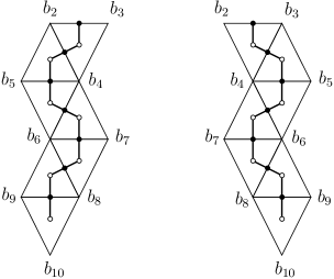
Figure 9. The path on the left is of cheapest descent. The path on the right is of cheapest descent if $b_{2}=b_{3}$.

First we examine lower bounds of bridge number as a function of depth. A bit of experimentation with Fibonacci functions shows that the fastest growth of depth relative to bridge number occurs for principal paths whose regular portions (i. e. the parts starting from $\tau_{m-2}$ and $\tau_{m-1}$) are the “paths of cheapest descent” seen in Figure 11. In that figure, the path on the left is always cheapest descent, and the one on the right is cheapest descent when $b_{2}=b_{3}$. Any principal path having more than two tunnels at a given depth will produce a larger bridge number, as will any principal path that emerges in the more costly direction out of a downward-pointing $2$-simplex. From Theorem 6.2 we now have:

Corollary 7.1.

Let $\tau$ be a regular tunnel of depth $d$, and in the principal path of $\tau$, let $\tau_{m}$ be the first tunnel of depth $2$, with principal vertex $\{\tau_{m-2},\tau_{m-1},\tau_{m}\}$. Put $b_{2}=\operatorname{br}(K_{\tau_{m-2}})$ and $b_{3}=\operatorname{br}(K_{\tau_{m-1}})$. For $n\geq 2$ let $b_{j}$ be given by the recursion

$$b_{2n}=b_{2n-1}+b_{2n-2}$$

$$b_{2n+1}=b_{2n}+b_{2n-2}$$

Then $\operatorname{br}(K_{\tau})\geq b_{2d}$.

We can now prove one of our main results.

Theorem 7.2 (Minimum Bridge Number).

For $d\geq 1$, the minimum bridge number of a knot having a tunnel of depth $d$ is given recursively by $a_{d}$, where $a_{1}=2$, $a_{2}=4$, and $a_{d}=2a_{d-1}+a_{d-2}$ for $d\geq 3$. Explicitly,

$$a_{d}=\frac{(1+\sqrt{2})^{d}}{\sqrt{2}}-\frac{(1-\sqrt{2})^{d}}{\sqrt{2}}\ .$$

and consequently ${\displaystyle\lim_{d\to\infty}}a_{d}-\frac{(1+\sqrt{2})^{d}}{\sqrt{2}}=0$.

Proof.

The smallest possible values for $\operatorname{br}(K_{\tau_{m-2}})$ and $\operatorname{br}(K_{\tau_{m-1}})$ in Corollary 7.1 are $2$. These occur for any $m$, since there are $2$-bridge knot tunnels with arbitrarily long cabling sequences, as seen in [5, Section 15]. Taking $b_{2}=b_{3}=2$ in Corollary 7.1 gives a $b_{2d}$ which is a general lower bound for the bridge number of a tunnel at depth $d$, and a little bit of algebra shows that $b_{2d}=a_{d}$ for the recursion in Theorem 7.2. As a matrix, the recursion is

$$\begin{bmatrix}a_{d+1}\\ a_{d}\end{bmatrix}=\begin{bmatrix}2&1\\ 1&0\end{bmatrix}\begin{bmatrix}a_{d}\\ a_{d-1}\end{bmatrix}\ .$$

The eigenvalues of this matrix are $1\pm\sqrt{2}$, and elementary linear algebra gives the formula $a_{d}=\frac{(1+\sqrt{2})^{d}}{\sqrt{2}}-\frac{(1-\sqrt{2})^{d}}{\sqrt{2}}$. ∎

We turn now to upper bounds. There is no upper bound in terms of depth, since there are depth $1$ tunnels with arbitrarily large bridge number, such as semisimple tunnels of torus knots [6]. We can, however, bound the bridge number of $K_{\tau}$ in terms of the number of cablings needed to produce $\tau$. This time, we use the principal path forced by choosing the larger of its two possible sums at every step, shown in Figure 10.

Figure 10. The fastest growing upper bounds for bridge number, starting with the last two semisimple tunnels in the cabling sequence.

Theorem 7.3 (Maximum Bridge Number).

Write the Fibonacci sequence $(1,1,2,3,\ldots)$ as $(F_{1},F_{2},\ldots)$. The maximum bridge number of a knot having a tunnel produced by $n$ cabling constructions, of which the first $m$ produce simple or semisimple tunnels, is $mF_{n-m+2}+F_{n-m+1}$.

Proof.

If $\tau$ is simple, then $\operatorname{br}(K_{\tau})=2$, $m=n=1$ and the expression $mF_{n-m+2}+F_{n-m+1}$ equals $2$. If $\tau$ is semisimple, then $m=n$ and $mF_{n-m+2}+F_{n-m+1}$ equals $m+1$, the upper bound given in Theorem 6.1. So we may assume that $\tau$ is regular.

In Figure 10, the top two vertices are $\tau_{m-2}$ and $\tau_{m-1}$, the last two semisimple tunnels that appear in the cabling sequence of $\tau_{n-1}$. There are semisimple tunnels $\tau_{m-1}$ produced by $m$ cabling constructions which have $\operatorname{br}(K_{\tau_{m-1}})=m+1$, such as the semisimple tunnels of the $(m+2,m+1)$ torus knot [6]. Therefore the maximum bridge number is that given by Theorem 6.2 applied to the principal path whose regular portion is shown in Figure 10. Using the fact that $m=m\cdot F_{1}$ and $m+1=m\cdot F_{2}+F_{1}$, one checks that this value is $mF_{n-m+2}+F_{n-m+1}$. ∎

Corollary 7.4.

The maximum bridge number of a knot having a tunnel produced by $n$ cabling operations is $F_{n+2}$.

Proof.

For a fixed $n$, the largest upper bound in Theorem 7.3 occurs when $m=2$. ∎

Proposition 8.3 below gives an explicit sequence of tunnels of torus knots that achieves the maximum value of Corollary 7.4.

8. Middle tunnels of torus knots

The tunnels of torus knots were classified by M. Boileau, M. Rost, and H. Zieschang [3] and independently by Y. Moriah [14].

For a $(p,q)$ torus knot $K_{p,q}$ contained in the standard torus $T$ in $S^{3}$, the middle tunnel is represented by an arc in $T$ that meets $K_{p,q}$ only in its endpoints. There are as many as two other tunnels, which always have depth $1$, but here we focus on the middle tunnels.

In this section, we will include some information on slope invariants, for those familiar with them. Slopes are not essential to the discussion, and can be ignored if the reader so chooses.

For the tunnels of torus knots, the slope and binary invariants were calculated in [6]. In particular, for the middle tunnels, we have the following theorem, in which $U=\begin{bmatrix}1&1\\ 0&1\end{bmatrix}$ and $L=\begin{bmatrix}1&0\\ 1&1\end{bmatrix}$:

Theorem 8.1.

Let $p$ and $q$ be relatively prime integers with $p>q\geq 2$. Write $p/q$ as a continued fraction $[n_{1},n_{2},\ldots,n_{k}]$ with all $n_{j}$ positive and $n_{k}\neq 1$. Let

$$A_{i}=\begin{cases}L&-n_{1}\leq i\leq-1\\ U&0\leq i\leq n_{2}-1\\ L&n_{2}\leq i\leq n_{2}+n_{3}-1\\ U&n_{2}+n_{3}\leq i\leq n_{2}+n_{3}+n_{4}-1\\ &\cdots\\ L&k\text{\ odd and\ }n_{2}+n_{3}+\cdots+n_{k-1}\leq i\leq n_{2}+n_{3}+\cdots+n_{k}-1\\ U&k\text{\ even and\ }n_{2}+n_{3}+\cdots+n_{k-1}\leq i\leq n_{2}+n_{3}+\cdots+n_{k}-1\ .\end{cases}$$

Put $N=n_{2}+n_{3}+\cdots+n_{k}-2$, and for $0\leq t\leq N$ put

$$\begin{bmatrix}a_{t}&b_{t}\\ c_{t}&d_{t}\end{bmatrix}=\prod_{i=t}^{-n_{1}}A_{i}\ ,$$

where the subscripts in the product occur in descending order. Then:

1. The middle tunnel of $K_{p/q}$ is produced by $N+1$ cabling constructions whose slopes $m_{0}$, $m_{1},\ldots\,$, $m_{N}$ are

   $$\left[\frac{1}{2n_{1}+1}\right],\;a_{1}d_{1}+b_{1}c_{1},\;a_{2}d_{2}+b_{2}c_{2},\;\ldots,\;a_{N}d_{N}+b_{N}c_{N}\ .$$

2. For each $t$, the cabling corresponding to the slope invariant $m_{t}$ produces the $(a_{t}+c_{t},b_{t}+d_{t})$ torus knot; in particular, the first cabling produces the $(2n_{1}+1,2)$ torus knot.

3. The binary invariants of the cabling sequence of this tunnel, for $2\leq t\leq N$, are given by $s_{t}=1$ if $A_{t}\neq A_{t-1}$ and $s_{t}=0$ otherwise.

Note that this enables one to find the invariants of the middle tunnels for all $(p,q)$ torus knots, since $K_{p,q}$ is isotopic to $K_{q,p}$ and $K_{p,-q}$ is equivalent to $K_{p,q}$ by an orientation-reversing homeomorphism taking middle tunnel to middle tunnel. Such an equivalence negates the slope invariants and does not change the binary invariants.

A bit of examination of the binary invariants yields a simple algorithm to find the depth of the middle tunnel of $K_{p,q}$, $p>q\geq 2$:

1. Write $p/q$ as a continued fraction $[n_{1},n_{2},\ldots,n_{k}]$ with all $n_{i}$ positive and $n_{k}\neq 1$.

2. Write the string $n_{2}\cdots n_{k}$ as $B_{1}B_{2}\cdots B_{\ell}$, where each $B_{i}$ is either $n_{i}n_{i+1}$ with $n_{i}=1$, or $n_{i}$ with $n_{i}\neq 1$.

3. The depth of the middle tunnel is $1+\ell$.

This is implemented in the software at [8].

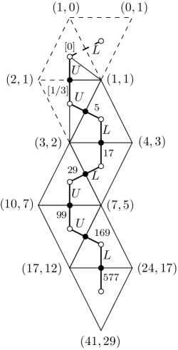
Figure 11. Slowest growth of bridge number as a function of depth for torus knot tunnels, corresponding to the continued fraction expansion $41/29=[1,2,2,2,2]$. The $(41,29)$ torus knot has the smallest bridge number of any torus knot with a depth $4$ tunnel.

Figure 11 shows an initial segment of the principal paths for the tunnels of the $(p,q)$-torus knots having continued fraction expansions of the form $p/q=[1,2,2,\ldots,2]$. Notice that this is the path of cheapest descent from Figure 9. The small numbers along the path are the slopes, the letters indicate whether the constructions correspond to multiplication by $U$ or by $L$, and the pairs show the $(p,q)$ for the torus knots determined by the tunnel at each step. The first nontrivial cabling, with $m_{0}=[1/3]$, produces a $(3,2)$-torus knot, and the second produces a $(4,3)$-torus knot with bridge number $3$. Since we always have $p>q$, the bridge number is simply the value of $q$. These obey the recursion of Corollary 7.1, starting with $b_{2}=2$ and $b_{3}=3$. Since the cabling sequence for the middle tunnel $\tau$ of any torus knot contains only one two-bridge knot (the $(2n_{1}+1,2)$-torus knot produced by the first nontrivial cabling), there is no regular torus knot tunnel which has $b_{3}=2$. Since the other tunnels of torus knots are semisimple, the maximum depth of any tunnel of a torus knot is the depth of its middle tunnel. Therefore each $b_{2d}$ in this sequence gives the minimum bridge number for a torus knot with a tunnel of depth $d$. This gives a version of the Minimum Bridge Number Theorem 7.2 for torus knot tunnels:

Theorem 8.2.

For $d\geq 1$, the minimum bridge number of a torus knot tunnel depth $d$ is given recursively by $t_{d}$, where $t_{1}=2$, $t_{2}=5$, and $t_{d}=2t_{d-1}+t_{d-2}$ for $d\geq 3$. Explicitly,

$$t_{d}=\frac{1}{2\sqrt{2}}(1+\sqrt{2})^{d+1}-\frac{1}{2\sqrt{2}}(1-\sqrt{2})^{d+1}\ ,$$

and consequently ${\displaystyle\lim_{d\to\infty}}t_{d}-\frac{1}{2\sqrt{2}}(1+\sqrt{2})^{d+1}=0$.

We note that $t_{d}$ is $a_{d+1}/2$, where $a_{d+1}$ is the lower bound in the Minimum Bridge Number Theorem 7.2. That is, the minimum bridge number of a torus knot having a tunnel of depth $d$ is exactly half the minimum bridge number for all knots having a tunnel of depth $d+1$, and is approximately $(1+\sqrt{2})/2$ times the minimum for all knots having a tunnel of depth $d$.

In fact, the middle tunnel any torus knot for which $p/q$ has an expansion $[n_{1},2,2,2,2,\ldots,2]$ will have a principal path as in the previous argument, since the first term in the continued fraction has no effect on the principal path. Middle tunnels for which the expansion is not of this form will have different principal paths, so we can state the following result:

Proposition 8.3.

The slowest growth of bridge number compared to depth for sequences of middle tunnels of torus knots occurs when the $p/q$ have continued fraction expansions of the form $\pm[n_{1},2,2,2,\ldots,2]$.

By similar considerations, one can obtain the upper bound version.

Proposition 8.4.

The fastest growth of bridge number of torus knots per number of cablings of the middle tunnels occurs for sequences of tunnels $\tau_{k}$ of $K_{p,q}$ for which the continued fraction expansions of $p/q$ are of the form $\pm[n_{1},1,1,1,\ldots,1]$, where there are $k$ $1$’s. For these tunnels, $K_{\tau_{k}}$ has bridge number $F_{k+2}$.

For these tunnels, the terminal part of the corridor is like that shown in Figure 10 with $m=2$. Since there are exactly $k$ cablings in the cabling sequence of $\tau_{k}$, these tunnels achieve the bridge numbers in the Maximum Bridge Number Theorem.

9. The case of tunnel number $1$ links

As explained in  [5], our entire theory of tunnel number $1$ knot tunnels can be adapted to include tunnels of tunnel number $1$ links, simply by adding the separating disks as possible slope disks. The full disk complex $\operatorname{{\mathcal{K}}}(H)$ is only slightly more complicated than $\operatorname{{\mathcal{D}}}(H)$. Each separating disk is disjoint from only two other disks, both nonseparating, so the additional vertices appear in $2$-simplices attached to $\operatorname{{\mathcal{D}}}(H)$ along the edge opposite the vertex that is a separating disk. The quotient $\operatorname{{\mathcal{K}}}(H)/\operatorname{{\mathcal{G}}}$ has only three types of additional $2$-simplices:

1. There is a unique orbit $\sigma_{0}$ of “primitive” separating disks, consisting of separating disks disjoint from a primitive pair, which are exactly the intersections of splitting spheres (see [16]) with $H$. In $\operatorname{{\mathcal{K}}}(H)/\operatorname{{\mathcal{G}}}$, $\sigma_{0}$ is a vertex of a “half-simplex” $\langle\sigma_{0},\pi_{0},\mu_{0}\rangle$ attached to $\operatorname{{\mathcal{D}}}(H)/\operatorname{{\mathcal{G}}}$ along $\langle\pi_{0},\mu_{0}\rangle$. It is the unique tunnel of the trivial $2$-component link.

2. Simple separating disks lie in half-simplices attached along $\langle\pi_{0},\mu_{0}\rangle$, just like nonseparating simple disks.

3. The remaining separating disks lie in $2$-simplices attached along edges of $\operatorname{{\mathcal{D}}}(H)/\operatorname{{\mathcal{G}}}$ spanned by two (orbits of) disks, at least one of which is nonprimitive.

For the spine, a single “Y” is added to $\operatorname{{\mathcal{T}}}$ for each added $2$-simplex as in (3), and a folded “Y” for each the half-simplices as in (1) and (2). The link in $\operatorname{{\mathcal{K}}}^{\prime}(H)/\operatorname{{\mathcal{G}}}$ of a link tunnel is simply the top edges (or top edge, for the trivial and simple tunnels) of such a “Y” (or folded “Y”).

The cabling operation differs only in allowing a separating slope disk, which produces a tunnel of a tunnel number $1$ link. The cabling sequence ends with the first separating slope disk. Thus the principal paths look exactly like those of the knot case, such as the one in Figure 4. The only difference is that no further continuation is possible if the final tunnel is the tunnel of a link.

For link tunnels, the distance and depth invariants are defined as for knot tunnels. Simple tunnels are the upper and lower tunnels of $2$-bridge links (and are the only tunnels of these links, see [1], [12], or [5, Theorem 16.3]). Depth $1$ tunnels are the tunnels of links with one component unknotted. The other component must be a $(1,1)$-knot, and the link must have torus bridge number $2$ [5, Theorem 16.4]. Lemma 3.1 holds when $\tau$ is separating, in fact the argument is an easier version of the argument in [11], so Theorem 3.3 and Corollary 3.5 hold for links as well as knots.

The Tunnel Leveling Addendum extends to tunnels of tunnel number $1$ links, since the efficient cabling construction of Section 5 works just as well in the link case. But the statement and proof are very much simpler, since only the level arc case need be considered.

Theorem 9.1 (Tunnel Leveling Addendum for Links).

Let $\tau$ be a tunnel of a tunnel number $1$ link, with principal vertex $\{\lambda,\rho,\tau\}$. Then $\operatorname{br}(K_{\tau})=\operatorname{br}(K_{\rho})+\operatorname{br}(K_{\lambda})$.

Using the Tunnel Leveling Addendum for Links, the computational results of Sections 6 and 7 hold as stated for tunnels of tunnel number $1$ links. Consequently, the software implementations of [8] also produce correct results for link tunnels.

References

- [1] C. Adams, A. Reid, Unknotting tunnels in two-bridge knot and link complements, Comment. Math. Helv. 71 (1996), 617–627.
- [2] E. Akbas, A presentation of the automorphisms of the -sphere that preserve a genus two Heegaard splitting, Pacific J. Math. 236 (2008), 201-222.
- [3] M. Boileau, M. Rost, and H. Zieschang, On Heegaard decompositions of torus knot exteriors and related Seifert fibre spaces, Math. Ann. 279 (1988), 553–581.
- [4] S. Cho, Homeomorphisms of the -sphere that preserve a genus Heegaard splitting, Proc. Amer. Math. Soc. 136 (2008), 1113–1123.
- [5] S. Cho and D. McCullough, The tree of knot tunnels, to appear in Geom. Top.
- [6] S. Cho and D. McCullough, Cabling sequences of tunnels of torus knots, to appear in Alg. Geom. Top.
- [7] S. Cho and D. McCullough, Constructing tunnels using giant steps, preprint.
- [8] S. Cho and D. McCullough, software available at www.math.ou.edu/dmccullough/ .
- [9] H. Goda, M. Ozawa, Makoto, and M. Teragaito, On tangle decompositions of tunnel number one links, J. Knot Theory Ramifications 8 (1999), 299–320.
- [10] H. Goda, M. Scharlemann, and A. Thompson, Levelling an unknotting tunnel, Geom. Topol. 4 (2000), 243–275.
- [11] J. Johnson, Bridge number and the curve complex, Mathematics ArXiv math.GT/0603102.
- [12] M. Kuhn, Tunnels of -bridge links, J. Knot Theory Ramifications 5 (1996), 167–171.
- [13] Y. Minsky, Y. Moriah, and S. Schleimer, High distance knots, Algebr. Geom. Topol. 7 (2007), 1471–1483.
- [14] Y. Moriah, Heegaard splittings of Seifert fibered spaces, Invent. Math. 91 (1988), 465–481.
- [15] K. Morimoto, M. Sakuma, On unknotting tunnels for knots, Math. Ann. 289 (1991), 143–167.
- [16] M. Scharlemann, Automorphisms of the 3-sphere that preserve a genus two Heegaard splitting, Bol. Soc. Mat. Mexicana (3) 10 (2004) 503–514.
- [17] M. Scharlemann and A. Thompson, Unknotting tunnels and Seifert surfaces, Proc. London Math. Soc. (3) 87 (2003), 523–544.
- [18] M. Scharlemann and M. Tomova, Alternate Heegaard genus bounds distance, Geom. Topol. 10 (2006), 593–617.