Cabling sequences of tunnels of torus knots

Abstract.

In previous work, we developed a theory of tunnels of tunnel number $1$ knots in $S^{3}$. It yields a parameterization in which each tunnel is described uniquely by a finite sequence of rational parameters and a finite sequence of $0$’s and $1$’s, that together encode a procedure for constructing the knot and tunnel. In this paper we calculate these invariants for all tunnels of torus knots.

Introduction

In previous work [4], we developed a theory of tunnels of tunnel number $1$ knots in $S^{3}$. It shows that every tunnel can be obtained from the unique tunnel of the trivial knot by a uniquely determined sequence of “cabling constructions”. A cabling construction is determined by a rational parameter, called its “slope,” so this leads to a parameterization of all tunnels of all tunnel number $1$ knots by sequences of rational numbers and “binary” invariants. Various applications of the theory are given in [4], [5] and [6], as well as other work in preparation.

Naturally, it is of interest to calculate these invariants for known examples of tunnels. In [4], they are calculated for all tunnels of $2$-bridge knots, and in the present paper we obtain them for all tunnels of torus knots. Tunnels of torus knots are a key example in our study of the “depth” invariant in [6]. Also, torus knots are special in that their complements have zero (Gromov) volume, so they should be critical to understanding how hyperbolic volumes of complements of tunnel number $1$ knots are related to the sequences of slope and binary invariants of their tunnels.

In the next section, we will give the main results. Sections 2, 3, and 4 provide a concise review of the parts of the theory from [4] that will be needed in this paper. The main results are proven in Section 5 for the middle tunnels and Section 6 for the upper and lower tunnels.

The calculations in this paper enable us to recover the classification of torus knot tunnels given by M. Boileau, M. Rost, and H. Zieschang [2] and Y. Moriah [8], although not their result that these are all the tunnels. We give this application in Section 7 below.

All of our algorithms to find the invariants are straightforward to implement computationally, and we have done this in software available at [7]. Sample computations are given in Section 1.

In work in progress, we are developing a general method for computing these invariants for all $(1,1)$-tunnels. In particular, this will recover the calculations for tunnels of $2$-bridge knots, given in [4], and for some of the tunnels of torus knots that we give here (the upper and lower tunnels, but not the middle tunnels). Still, we think it is worthwhile to give the method of this paper, which is more direct and more easily visualized.

We are grateful to the referee for a prompt and careful reading of the original manuscript.

1. The main results

To set notation, consider a (nontrivial) $(p,q)$ torus knot $K_{p,q}$, contained in a standard torus $T$ bounding a solid torus $V\subset S^{3}$. In $\pi_{1}(V)$, $K_{p,q}$ represents $p$ times a generator. The complementary torus $\overline{S^{3}-V}$ will be denoted by $W$.

The tunnels of torus knots were classified by M. Boileau, M. Rost, and H. Zieschang [2] and Y. Moriah [8]. The middle tunnel of $K_{p,q}$ is represented by an arc in $T$ that meets $K_{p,q}$ only in its endpoints. The upper tunnel of $K_{p,q}$ is represented by an arc $\alpha$ properly imbedded in $W$, such that the circle which is the union of $\alpha$ with one of the two arcs of $K_{p,q}$ with endpoints equal to the endpoints of $\alpha$ is a deformation retract of $W$. The lower tunnel is like the upper tunnel, but interchanging the roles of $V$ and $W$. In certain cases, some of these tunnels are equivalent, as we will detail in Section 7.

To state our results for the middle tunnels, assume for now that $p,q>1$. Since $K_{p,q}$ and $K_{q,p}$ are equivalent by an orientation-preserving homeomorphism of $S^{3}$ taking middle tunnel to middle tunnel, we may also assume that $p>q$. Put $U=\begin{pmatrix}1&1\\ 0&1\end{pmatrix}$ and $L=\begin{pmatrix}1&0\\ 1&1\end{pmatrix}$.

Theorem 1.1.

Let $p$ and $q$ be relatively prime integers with $p>q\geq 2$. Write $p/q$ as a continued fraction $[n_{1},n_{2},\ldots,n_{k}]$ with all $n_{j}$ positive and $n_{k}\neq 1$. Let

$$A_{i}=\begin{cases}L&-n_{1}\leq i\leq-1\\ U&0\leq i\leq n_{2}-1\\ L&n_{2}\leq i\leq n_{2}+n_{3}-1\\ U&n_{2}+n_{3}\leq i\leq n_{2}+n_{3}+n_{4}-1\\ &\cdots\\ L&k\text{\ odd and\ }n_{2}+n_{3}+\cdots+n_{k-1}\leq i\leq n_{2}+n_{3}+\cdots+n_{k}-1\\ U&k\text{\ even and\ }n_{2}+n_{3}+\cdots+n_{k-1}\leq i\leq n_{2}+n_{3}+\cdots+n_{k}-1\ .\end{cases}$$

Put $N=n_{2}+n_{3}+\cdots+n_{k}-2$, and for $0\leq t\leq N$ put

$$\begin{pmatrix}a_{t}&b_{t}\\ c_{t}&d_{t}\end{pmatrix}=\prod_{i=t}^{-n_{1}}A_{i}\ ,$$

where the subscripts in the product occur in descending order. Then:

1. The middle tunnel of $K_{p/q}$ is produced by $N+1$ cabling constructions whose slopes $m_{0}$, $m_{1},\ldots\,$, $m_{N}$ are

   $$\left[\frac{1}{2n_{1}+1}\right],\;a_{1}d_{1}+b_{1}c_{1},\;a_{2}d_{2}+b_{2}c_{2},\;\ldots,\;a_{N}d_{N}+b_{N}c_{N}\ .$$

2. For each $t$, the cabling corresponding to the slope invariant $m_{t}$ produces the $(a_{t}+c_{t},b_{t}+d_{t})$ torus knot; in particular, the first cabling produces the $(2n_{1}+1,2)$ torus knot.

3. The binary invariants of the cabling sequence of this tunnel, for $2\leq t\leq N$, are given by $s_{t}=1$ if $A_{t}\neq A_{t-1}$ and $s_{t}=0$ otherwise.

If $pq<0$, then $K_{p,q}$ is equivalent to $K_{|p|,|q|}$ by an orientation-reversing homeomorphism taking the middle tunnel to the middle tunnel, so the cabling slopes for the middle tunnel of $K_{p,q}$ are just the negatives of those of $K_{|p|,|q|}$ given in Theorem 1.1, while the binary invariants are unchanged.

It is not difficult to implement this calculation computationally, and we have made a script for this available [7]. For $K_{41,29}$, we find

TorusKnots$>$ middleSlopes(41, 29)
[ 1/3 ], 5, 17, 29, 99, 169, 577

and for $K_{181,-48}$

TorusKnots$>$ middleSlopes(181, -48)
[ 6/7 ], -15, -23, -31, -151, -271, -883, -2157, -3431

The torus knots that are the intermediate knots in the cabling sequence are found by

TorusKnots> intermediates( 41, 29 )
(3,2), (4,3), (7,5), (10,7), (17,12), (24,17), (41,29)

and the binary invariants by

TorusKnots> binaries(41, 29)
[1, 0, 1, 0, 1]

Now we consider the upper and lower tunnels. Since these are semisimple tunnels, their binary invariants $s_{i}$ are all $0$ (see Section 4). The cabling slopes are given as follows.

Theorem 1.2.

Let $p$ and $q$ be relatively prime integers, both greater than $1$. For integers $k$ with $1\leq k\leq q$, define integers $p_{k}$ by

$$p_{k}=\lceil kp/q\rceil=\min\{j\;|\;jq/p\geq k\}\ ,$$

and let $k_{0}=\min\{k\;|\;p_{k}>1\}$. Then the upper tunnel of $K_{p,q}$ is produced by $q-k_{0}$ cabling operations, whose slopes are

$$[1/(2p_{k_{0}}-1)],\;2p_{k_{0}+1}-1,\;\ldots\,,\;2p_{q-1}-1\ .$$

As before, when $pq<0$ the slopes are just the negatives of those given in Theorem 1.2 for $K_{|p|,|q|}$. The lower tunnel of $K_{p,q}$ is equivalent to the upper tunnel of $K_{q,p}$, so Theorem 1.2 also finds the slope sequences of all lower tunnels.

Again, this algorithm is easily scripted and is available at [7]. Sample calculations are:

TorusKnots$>$ upperSlopes( 18, 7 )
[ 1/ 5 ], 11, 15, 21, 25, 31

TorusKnots$>$ upperSlopes( 7, 18 )
[ 1/ 3 ], 3, 3, 5, 5, 7, 7, 7, 9, 9, 11, 11, 11, 13, 13

TorusKnots$>$ lowerSlopes( 18, 7 )
[ 1/ 3 ], 3, 3, 5, 5, 7, 7, 7, 9, 9, 11, 11, 11, 13, 13

Theorems 1.1 and 1.2 show immediately the following integrality result:

Corollary 1.3.

Let $\tau$ be a tunnel of a torus knot. Then the first slope invariant $m_{0}$ of $\tau$ is of the form $[1/n]$ for some odd integer $n$, and all other slopes are odd integers.

For the middle tunnels, the integrality of the slope invariants $m_{i}$ for $i\geq 1$ follows from the work of Scharlemann and Thompson [10] (which inspired our work in [4]). For as shown in [4, Section 14], their invariant $\rho(\tau)$ is our final (or “principal”) slope invariant $m_{N}$ reduced modulo $2$ (that is, viewed as an element of $\operatorname{{\mathbb{Q}}}/2\operatorname{{\mathbb{Z}}}$). Scharlemann and Thompson computed that the $\rho$-invariants of the middle tunnels are $1$, so it follows that $m_{N}$ must be an odd integer. As our construction in Section 5 will show, the intermediate slope invariants $m_{i}$ are principal slope invariants for middle tunnels of other torus knots, so they too must be odd integers.

2. Tunnels as disks

This section gives a brief overview of the theory in [4]. Fix a standard unknotted handlebody $H$ in $S^{3}$. Regard a tunnel of $K$ as a $1$-handle attached to a neighborhood of $K$ to obtain an unknotted genus-$2$ handlebody. Moving this handlebody to $H$, a cocore disk for the $1$-handle moves to a nonseparating disk in $H$. The indeterminacy due to the choice of isotopy is exactly the Goeritz group $\operatorname{{\mathcal{G}}}$, studied in [1, 3, 9]. Consequently, the collection of all tunnels of all tunnel number $1$ knots, up to orientation-preserving homeomorphism, corresponds to the orbits of nonseparating disks in $H$ under the action of $\operatorname{{\mathcal{G}}}$. From [1, 3, 9], the action can be understood and the equivalence classes, i.e. the tunnels, arranged in a treelike structure which encodes much of the topological structure of tunnel number $1$ knots and their tunnels.

When a nonseparating disk $\tau\subset H$ is regarded as a tunnel, the corresponding knot is a core circle of the solid torus that results from cutting $H$ along $\tau$. This knot is denoted by $K_{\tau}$.

A disk $\tau$ in $H$ is called primitive if there is a disk $\tau^{\prime}$ in $\overline{S^{3}-H}$ such that $\partial\tau$ and $\partial\tau^{\prime}$ cross in one point in $\partial H$. Equivalently, $K_{\tau}$ is the trivial knot in $S^{3}$. All primitive disks are equivalent under the action of $\operatorname{{\mathcal{G}}}$. This equivalence class is the unique tunnel of the trivial knot.

A primitive pair is an isotopy class of two disjoint nonisotopic primitive disks in $H$. A primitive triple is defined similarly.

3. Slope disks and cabling arcs

This section gives the definitions needed for computing slope invariants. Fix a pair of nonseparating disks $\lambda$ and $\rho$ (for “left” and “right”) in the standard unknotted handlebody $H$ in $S^{3}$, as shown abstractly in Figure 1. The pair $\{\lambda,\rho\}$ is arbitrary, so in the true picture in $H$ in $S^{3}$, they will typically look a great deal more complicated than the pair shown in Figure 1. Let $N$ be a regular neighborhood of $\lambda\cup\rho$ and let $B$ be the closure of $H-N$. The frontier of $B$ in $H$ consists of four disks which appear vertical in Figure 1. Denote this frontier by $F$, and let $\Sigma$ be $B\cap\partial H$, a sphere with four holes.

2pt $\lambda$ [B] at -18 136 $\rho$ [B] at 595 136

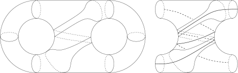
Figure 1. A slope disk of $\{\lambda,\rho\}$, and a pair of its cabling arcs contained in $B$.

A slope disk for $\{\lambda,\rho\}$ is an essential disk in $H$, possibly separating, which is contained in $B-F$ and is not isotopic to any component of $F$. The boundary of a slope disk always separates $\Sigma$ into two pairs of pants, conversely any loop in $\Sigma$ that is not homotopic into $\partial\Sigma$ is the boundary of a unique slope disk. (Throughout our work, “unique” means unique up to isotopy in an appropriate sense.) If two slope disks are isotopic in $H$, then they are isotopic in $B$.

An arc in $\Sigma$ whose endpoints lie in two different boundary circles of $\Sigma$ is called a cabling arc. Figure 1 shows a pair of cabling arcs disjoint from a slope disk. A slope disk is disjoint from a unique pair of cabling arcs, and each cabling arc determines a unique slope disk.

Each choice of nonseparating slope disk for a pair $\mu=\{\lambda,\rho\}$ determines a correspondence between $\operatorname{{\mathbb{Q}}}\cup\{\infty\}$ and the set of all slope disks of $\mu$, as follows. Fixing a nonseparating slope disk $\tau$ for $\mu$, write $(\mu;\tau)$ for the ordered pair consisting of $\mu$ and $\tau$.

Definition 3.1.

A perpendicular disk for $(\mu;\tau)$ is a disk $\tau^{\perp}$, with the following properties:

1. $\tau^{\perp}$ is a slope disk for $\mu$.

2. $\tau$ and $\tau^{\perp}$ intersect transversely in one arc.

3. $\tau^{\perp}$ separates $H$.

There are infinitely many choices for $\tau^{\perp}$, but because $H\subset S^{3}$ there is a natural way to choose a particular one, which we call $\tau^{0}$. It is illustrated in Figure 2. To construct it, start with any perpendicular disk and change it by Dehn twists of $H$ about $\tau$ until the core circles of the complementary solid tori have linking number $0$ in $S^{3}$.

2pt $\lambda^{+}$ [B] at 148 298 $\rho^{+}$ [B] at 437 300 $\lambda^{-}$ [B] at 149 -25 $\rho^{-}$ [B] at 433 -21 $\lambda$ [B] at -15 140 $\tau$ [B] at 376 141 $\rho$ [B] at 594 140 $K_{\rho}$ [B] at 210 222 $K_{\lambda}$ [B] at 369 222 $\tau^{0}$ [B] at 291 298

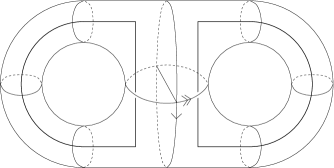
Figure 2. The slope-zero perpendicular disk $\tau^{0}$. It is chosen so that $K_{\lambda}$ and $K_{\rho}$ have linking number $0$.

For calculations, it is convenient to draw the picture as in Figure 2, and orient the boundaries of $\tau$ and $\tau^{0}$ so that the orientation of $\tau^{0}$ (the “$x$-axis”), followed by the orientation of $\tau$ (the “$y$-axis”), followed by the outward normal of $H$, is a right-hand orientation of $S^{3}$. At the other intersection point, these give the left-hand orientation, but the coordinates are unaffected by changing the choices of which of $\{\lambda,\rho\}$ is $\lambda$ and which is $\rho$, or changing which of the disks $\lambda^{+}$, $\lambda^{-}$, $\rho^{+}$, and $\rho^{-}$ are “$+$” and which are “$-$”, provided that the “$+$” disks both lie on the same side of $\lambda\cup\rho\cup\tau$ in Figure 2.

Let $\widetilde{\Sigma}$ be the covering space of $\Sigma$ such that:

1. $\widetilde{\Sigma}$ is the plane with an open disk of radius $1/8$ removed from each point with coordinates in $\operatorname{{\mathbb{Z}}}\times\operatorname{{\mathbb{Z}}}+(\frac{1}{2},\frac{1}{2})$.

2. The components of the preimage of $\tau$ are the vertical lines with integer $x$-coordinate.

3. The components of the preimage of $\tau^{0}$ are the horizontal lines with integer $y$-coordinate.

Figure 3 shows a picture of $\widetilde{\Sigma}$ and a fundamental domain for the action of its group of covering transformations, which is the orientation-preserving subgroup of the group generated by reflections in the half-integer lattice lines (that pass through the centers of the missing disks). Each circle of $\partial\widetilde{\Sigma}$ double covers a circle of $\partial\Sigma$.

2pt $\lambda^{+}$ [B] at 65 66 $\lambda^{-}$ [B] at 138 66 $\lambda^{+}$ [B] at 209 66 $\lambda^{-}$ [B] at 281 66 $\rho^{+}$ [B] at 65 142 $\rho^{-}$ [B] at 138 142 $\rho^{+}$ [B] at 209 142 $\rho^{-}$ [B] at 281 142 $\lambda^{+}$ [B] at 65 210 $\lambda^{-}$ [B] at 138 210 $\lambda^{+}$ [B] at 209 210 $\lambda^{-}$ [B] at 281 210 $\rho^{+}$ [B] at 65 286 $\rho^{-}$ [B] at 138 286 $\rho^{+}$ [B] at 209 286 $\rho^{-}$ [B] at 281 286 $\lambda^{+}$ [B] at 420 0 $\lambda^{-}$ [B] at 740 0 $\rho^{+}$ [B] at 420 310 $\rho^{-}$ [B] at 745 309 $\tau^{0}$ [B] at 738 158 $\tau$ [B] at 578 244

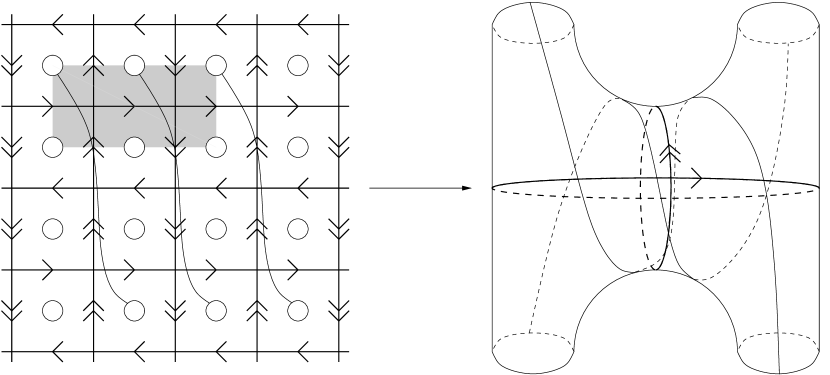
Figure 3. The covering space $\widetilde{\Sigma}\to\Sigma$, and some lifts of a pair of $[1,-3]$-cabling arcs. The shaded region is a fundamental domain.

Each lift of a cabling arc $\alpha$ of $\Sigma$ to $\widetilde{\Sigma}$ runs from a boundary circle of $\widetilde{\Sigma}$ to one of its translates by a vector $(p,q)$ of signed integers, defined up to multiplication by the scalar $-1$. In this way $\alpha$ receives a slope pair $[p,q]=\{(p,q),(-p,-q)\}$, and is called a $[p,q]$-cabling arc. The corresponding slope disk is assigned the slope pair $[p,q]$ as well.

An important observation is that a $[p,q]$-slope disk is nonseparating in $H$ if and only if $q$ is odd. Both happen exactly when a corresponding cabling arc has one endpoint in $\lambda^{+}$ or $\lambda^{-}$ and the other in $\rho^{+}$ or $\rho^{-}$.

Definition 3.2.

Let $\lambda$, $\rho$, and $\tau$ be as above, and let $\mu=\{\lambda,\rho\}$. The $(\mu;\tau)$-slope of a $[p,q]$-slope disk or cabling arc is $q/p\in\operatorname{{\mathbb{Q}}}\cup\{\infty\}$.

The $(\mu;\tau)$-slope of $\tau^{0}$ is $0$, and the $(\mu;\tau)$-slope of $\tau$ is $\infty$.

Slope disks for a primitive pair are called simple disks, and are handled in a special way. Rather than using a particular choice of $\tau$ from the context, one chooses $\tau$ to be some third primitive disk. Altering this choice can change $[p,q]$ to any $[p+nq,q]$, but the quotient $p/q$ is well-defined as an element of $\operatorname{{\mathbb{Q}}}/\operatorname{{\mathbb{Z}}}\cup\{\infty\}$. This element $[p/q]$ is called the simple slope of the slope disk. The simple slope is $[0]$ exactly when the slope disk is itself primitive, and has $q$ odd exactly when the simple disk is nonseparating. Simple disks have the same simple slope exactly when they are equivalent by an element of the Goeritz group.

4. The cabling construction

In a sentence, the cabling construction is to “Think of the union of $K$ and the tunnel arc as a $\theta$-curve, and rationally tangle the ends of the tunnel arc and one of the arcs of $K$ in a neighborhood of the other arc of $K$.” We sometimes call this “swap and tangle,” since one of the arcs in the knot is exchanged for the tunnel arc, then the ends of other arc of the knot and the tunnel arc are connected by a rational tangle.

Figure 4 illustrates two cabling constructions, one starting with the trivial knot and obtaining the trefoil, then another starting with the tunnel of the trefoil.

2pt $\pi_{0}$ [B] at -7 178 $\pi$ [B] at 65 178 $\pi_{1}$ [B] at 120 178 $\pi_{0}$ [B] at 177 178 $\tau_{0}$ [B] at 239 227 $\pi_{1}$ [B] at 304 177 $\pi_{1}$ [B] at 66 121 $\tau_{0}$ [B] at 127 93 $\pi_{0}$ [B] at 93 39 $\tau_{1}$ [B] at 226 54 $\pi_{0}$ [B] at 250 32 $\tau_{0}$ [B] at 290 99

Figure 4. Examples of the cabling construction.

More precisely, begin with a triple $\{\lambda,\rho,\tau\}$, regarded as a pair $\mu=\{\lambda,\rho\}$ with a slope disk $\tau$. Choose one of the disks in $\{\lambda,\rho\}$, say $\lambda$, and a nonseparating slope disk $\tau^{\prime}$ of the pair $\{\lambda,\tau\}$, other than $\rho$. This is a cabling operation producing the tunnel $\tau^{\prime}$ from $\tau$. In terms of the “swap and tangle” description of a cabling, $\lambda$ is dual to the arc of $K_{\tau}$ that is retained, and the slope disk $\tau^{\prime}$ determines a pair of cabling arcs that form the rational tangle that replaces the arc of $K_{\tau}$ dual to $\rho$.

Provided that $\{\lambda,\rho,\tau\}$ was not a primitive triple, we define the slope of this cabling operation to be the $(\{\lambda,\tau\};\rho)$-slope of $\tau^{\prime}$. When $\{\lambda,\rho,\tau\}$ is primitive, the cabling construction starts with the tunnel of the trivial knot and produces an upper or lower tunnel of a $2$-bridge knot, unless $\tau^{\prime}$ is primitive, in which case it is again the tunnel of the trivial knot and the cabling is called trivial. The slope of a cabling starting with a primitive triple is defined to be the simple slope of $\tau^{\prime}$. The cabling is trivial when the simple slope is $[0]$.

Theorem 13.2 of [4] shows that every tunnel of every tunnel number $1$ knot can be obtained by a uniquely determined sequence of cabling constructions. The associated cabling slopes form a sequence

$$m_{0},\;m_{1},\;\cdots\;,\;m_{n}=[p_{0}/q_{0}],\;q_{1}/p_{1},\;\cdots\;,\;q_{n}/p_{n}$$

where $m_{0}\in\operatorname{{\mathbb{Q}}}/\operatorname{{\mathbb{Z}}}$ and each $q_{i}$ is odd.

There is a second set of invariants associated to a tunnel. Each $m_{i}$ is the slope of a cabling that begins with a triple of disks $\{\lambda_{i-1},\rho_{i-1},\tau_{i-1}\}$ and finishes with $\{\lambda_{i},\rho_{i},\tau_{i}\}$. For $i\geq 2$, put $s_{i}=1$ if $\{\lambda_{i},\rho_{i},\tau_{i}\}=\{\tau_{i-2},\tau_{i-1},\tau_{i}\}$, and $s_{i}=0$ otherwise. In terms of the swap-and-tangle construction, the invariant $s_{i}$ is $1$ exactly when the rational tangle replaces the arc that was retained by the previous cabling (for $i=1$, the choice does not matter, as there is an element of the Goeritz group that preserves $\tau_{0}$ and interchanges $\lambda_{0}$ and $\rho_{0}$).

In the sequence of triples described in the previous paragraph, the disks $\lambda_{i}$ and $\rho_{i}$ form the principal pair for the tunnel $\tau_{i}$. They are the disks called $\mu^{+}$ and $\mu^{-}$ in [10].

A nontrivial tunnel $\tau_{0}$ produced from the tunnel of the trivial knot by a single cabling construction is called a simple tunnel. As already noted, these are the “upper and lower” tunnels of $2$-bridge knots. Not surprisingly, the simple slope $m_{0}$ is a version of the standard rational parameter that classifies the $2$-bridge knot $K_{\tau_{0}}$.

A tunnel is called semisimple if it is disjoint from a primitive disk, but not from any primitive pair. The simple and semisimple tunnels are exactly the $(1,1)$-tunnels, that is, the upper and lower tunnels of knots in $1$-bridge position with respect to a Heegaard torus of $S^{3}$. A tunnel is semisimple if and only if all $s_{i}=0$. The reason is that both conditions characterize cabling sequences in which one of the original primitive disks is retained in every cabling; this corresponds to the fact that the union of the tunnel arc and one of the arcs of the knot is unknotted.

A tunnel is called regular if it is neither primitive, simple, or semisimple.

5. The middle tunnels

2pt $q$ [B] at -3 85 $q-(qq^{\prime}-1)/p$ [B] at -29 74 $(qq^{\prime}-1)/p$ [B] at -21 14 $\lambda$ [B] at 33 28 $\tau$ [B] at 60 25 $\rho$ [B] at 79 53 $q^{\prime}$ [B] at 56 -5 $p-q^{\prime}$ [B] at 89 -5 $p$ [B] at 139 -5 $(p,q)$ [B] at 140 90 $\lambda$ [B] at 191 38 $\rho$ [B] at 218 58 $\tau$ [B] at 224 38 $K_{\lambda}$ [B] at 210 12 $K_{\rho}$ [B] at 242 36

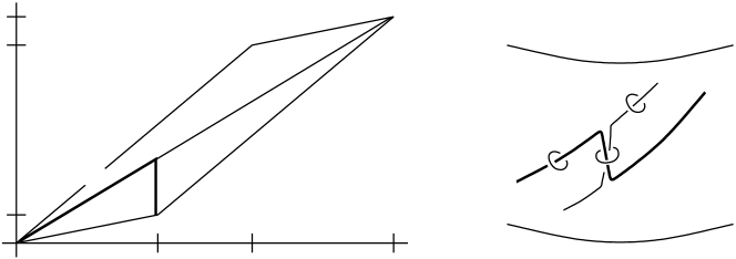
Figure 5. The properties of $q^{\prime}$. The darker segments correspond to $K_{\rho}$, a $(q^{\prime},(qq^{\prime}-1)/p)$ torus knot. The picture on the right shows $K_{\lambda}$ in the torus $T\subset S^{3}$, and $K_{\rho}$ pulled slightly outside of $T$.

In this section we will prove Theorem 1.1. We have relatively prime integers $p>q\geq 2$, and we use the notations $T$, $V$, and $W$ of Section 1.

First we examine a cabling operation that takes the middle tunnel $\tau$ and produces a middle tunnel of a new torus knot. Let $q^{\prime}$ be the integer with $0<q^{\prime}<p$ such that $qq^{\prime}\equiv 1\pmod{p}$. If the principal pair $\{\lambda,\rho\}$ of $\tau$ is positioned as shown in Figures 5 and 6 (our inductive construction of these tunnels will show that the pair shown in the figures is indeed the principal pair), then $K_{\rho}$ is a $(q^{\prime},(qq^{\prime}-1)/p)$ torus knot, and $K_{\lambda}$ is a $(p-q^{\prime},q-(qq^{\prime}-1)/p)$ torus knot. We set $(p_{1},q_{1})=(q^{\prime},(qq^{\prime}-1)/p)$ and $(p_{2},q_{2})=(p-q^{\prime},q-(qq^{\prime}-1)/p)$, so that $K_{\rho}$ and $K_{\lambda}$ are respectively the $(p_{1},q_{1})$ and $(p_{2},q_{2})$ torus knots.

In Figure 5, the linking number of $K_{\rho}$ with $K_{\lambda}$, up to sign conventions, is $q_{1}p_{2}$. One way to see this is to note that a Seifert surface for $K_{\lambda}$ can be constructed using $q_{2}$ meridian disks of $V$ and $p_{2}$ meridian disks of $W$ (by attaching bands contained in a small neighborhood of $T$). When $K_{\rho}$ is pulled slightly outside of $V$, as indicated in Figure 5, it has $q_{1}$ intersections with each of the $p_{2}$ meridian disks of $W$, all crossing the disks in the same direction.

2pt $\lambda$ [B] at 45 290 $\rho$ [B] at 263 458 $K_{\tau^{\prime}}$ [B] at 90 265 $\tau^{\prime}$ [B] at 137 295 $\tau$ [B] at 243 298 $\tau^{\prime}$ [B] at 213 211 $K_{\tau^{\prime}}$ [B] at 308 238 $\lambda^{+}$ [B] at 423 288 $\rho^{0}$ [B] at 483 329 $\rho$ [B] at 639 457 $\tau^{+}$ [B] at 623 309 $\tau^{-}$ [B] at 623 270 $qp_{2}$ [B] at 474 16 $\lambda^{-}$ [B] at 659 179

Figure 6. The cabling construction that replaces $\rho$ (compare with Figure 2) with $\tau^{\prime}$. The left drawing shows the new tunnel disk $\tau^{\prime}$ and the knot $K_{\tau^{\prime}}$. The right drawing shows a cabling arc for $\tau^{\prime}$, running from $\lambda^{+}$ to $\tau^{-}$, and the disks $\rho$ and $\rho^{0}$ used to calculate its slope.

Figure 6 shows the new tunnel disk $\tau^{\prime}$ for a cabling construction that produces a $(p+p_{2},q+q_{2})$ torus knot $K_{\tau^{\prime}}$. This disk meets $T$ perpendicularly. The drawing on the right in Figure 6 illustrates the setup for the calculation of the $(\{\lambda,\tau\};\rho)$-slope pair of $\tau^{\prime}$. The $qp_{2}$ turns of $\rho^{0}$, with the case $qp_{2}=2$ drawn in the figure, make the copies of $K_{\tau}=K_{p,q}$ and $K_{\lambda}=K_{p_{2},q_{2}}$ in its complement have linking number $0$. A cabling arc for $\tau^{\prime}$ is shown. Examination of its crossings with $\partial\rho$ and $\partial\rho^{0}$ shows that the slope pair of $\tau^{\prime}$ is $[1,2qp_{2}+1]$.

Put $U=\begin{pmatrix}1&1\\ 0&1\end{pmatrix}$ and $L=\begin{pmatrix}1&0\\ 1&1\end{pmatrix}$. If $K_{1}$ is a $(p_{1},q_{1})$ torus knot and $K_{2}$ is a $(p_{2},q_{2})$ torus knot, we denote by $M(K_{1},K_{2})$ the matrix $\begin{pmatrix}p_{1}&q_{1}\\ p_{2}&q_{2}\end{pmatrix}$. In our case, this is the matrix $M(K_{\rho},K_{\lambda})$. Adding the rows of $M(K_{\rho},K_{\lambda})$ gives $(p,q)$, corresponding to $K_{\tau}$, so

$$M(K_{\tau},K_{\lambda})=U\cdot M(K_{\rho},K_{\lambda})\ .$$

The left drawing of Figure 6 can be repositioned by isotopy so that $\lambda$, $\tau$, and $\tau^{\prime}$ look respectively as did $\lambda$, $\rho$, and $\tau$ in the original picture, with $\tau^{\prime}$ as the tunnel of the $(p+p_{2},q+q_{2})$ torus knot. Thus the procedure can be repeated, each time multiplying the matrix by another factor of $U$.

2pt $\lambda$ [B] at 20 280 $\rho^{-}$ [B] at 271 476 $\lambda^{0}$ [B] at 230 335 $\tau^{-}$ [B] at 150 257 $\tau^{+}$ [B] at 150 218 $\rho^{+}$ [B] at 34 4 $pq_{1}$ [B] at 276 181

Figure 7. Calculation of the slope of $\tau^{\prime}$ for a cabling construction replacing $\lambda$. The cabling arc runs from $\rho^{-}$ to $\tau^{+}$.

Figure 7 illustrates the similar calculation of the slope of the cabling construction replacing $\lambda$ by a new tunnel $\tau^{\prime}$. This produces a $(p+p_{1},q+q_{1})$ torus knot. In this case we have

$$M(K_{\rho},K_{\tau})=L\cdot M(K_{\rho},K_{\lambda})\ .$$

The slope pair of $\tau^{\prime}$ is $[1,2qp_{1}-1]$. One might expect $2qp_{1}+1$ as the second term, in analogy with the construction replacing $\rho$. However, as seen in Figure 7, the $pq_{1}$ twists needed in $\lambda^{0}$ are in the same direction as the twists in the calculation for $\rho$, not in the mirror-image sense. This results in two fewer crossings of the cabling arc for $\tau^{\prime}$ with $\lambda^{0}$ than before. In fact, the slope pairs for the two constructions can be described in a uniform way: For either of the matrices $M(K_{\tau},K_{\lambda})$ and $M(K_{\rho},K_{\tau})$, a little bit of arithmetic shows that the second entry of the slope pair for the cabling operation that produced them is the sum of the product of the diagonal entries and the product of the off-diagonal entries, that is, $[1,pq_{2}+qp_{2}]$ in the first case and $[1,pq_{1}+qp_{1}]$ in the second.

We can now describe the complete cabling sequence. Still assuming that $p$ and $q$ are both positive and $p>q$, write $p/q$ as $[n_{1},n_{2},\ldots,n_{k}]$ with all $n_{i}$ positive. We may assume that $n_{k}\neq 1$. According as $k$ is even or odd, we consider the product $U^{n_{k}}L^{n_{k-1}}\cdots U^{n_{2}}L^{n_{1}}$ or $L^{n_{k}}U^{n_{k-1}}\cdots U^{n_{2}}L^{n_{1}}$.

Start with a trivial knot regarded as a $(1,1)$ torus knot, and the “middle” tunnel $\tau$ in $T$. For the disks $\lambda$ and $\rho$ shown in Figure 6, $K_{\rho}$ is a $(1,0)$ torus knot and $K_{\lambda}$ is a $(0,1)$ torus knot. For this positioning of the trivial knot, the disks $\lambda$, $\rho$, and $\tau$ are all primitive, so $\{\lambda,\rho\}$ may be regarded as the principal pair for the tunnel $\tau$. Cablings of the two types above will preserve the fact that the pair $\{\lambda,\rho\}$ shown in Figure 6 is the principal pair.

At this point, the matrix $M(K_{\rho},K_{\lambda})$ is the identity matrix. Multiplying by $L^{n_{1}}$ corresponds to doing $n_{1}$ cabling constructions of the second type described above (replacing $\lambda$). These cablings have slope $[1]=[0]\in\operatorname{{\mathbb{Q}}}/\operatorname{{\mathbb{Z}}}$, so are trivial cablings, but their effect is to produce the trivial knot positioned as an $(n_{1}+1,1)$ torus knot. At that stage, $M(K_{\rho},K_{\lambda})$ is $\begin{pmatrix}1&0\\ n_{1}&1\end{pmatrix}$, which is the matrix $M_{-1}$ in the statement of Theorem 1.1. Then, multiplying by $U$ corresponds to a nontrivial cabling construction of the first type (replacing $\rho$). The new matrix $M(K_{\tau},K_{\lambda})$ is $\begin{pmatrix}n_{1}+1&1\\ n_{1}&1\end{pmatrix}$, or in the notation of Theorem 1.1, $M_{0}$, and the knot $K_{\tau^{\prime}}$ is a $(2n_{1}+1,2)$ torus knot. As explained above, the construction has slope pair $[1,2n_{1}+1]$, so the simple slope is $m_{0}=[1/(2n_{1}+1)]$. Continue by multiplying $n_{2}-1$ additional times by $U$, then $n_{3}$ times by $L$ and so on, performing additional cabling constructions with slopes calculated as above from the matrices of the current $K_{\rho}$, $K_{\lambda}$, and $K_{\tau}$. This produces the sequence of matrices $M_{t}$ in Theorem 1.1 and the corresponding slope invariants $m_{t}=a_{t}d_{t}+b_{t}c_{t}$.

At the end, there is no cabling construction corresponding to the last factor $L$ or $U$. For specificity, suppose $k$ was even and the product was $U^{n_{k}}L^{n_{k-1}}\cdots U^{n_{1}}L^{n_{1}}$. At the last stage, we apply $n_{k}-1$ cabling constructions corresponding to multiplications by $U$, and arrive at a tunnel $\tau$ for which $M(K_{\rho},K_{\lambda})$ is $U^{n_{k}-1}L^{n_{k-1}}\cdots U^{n_{2}}L^{n_{1}}=M_{N}$. The sum of the rows is then $(p,q)$ (multiplying by $U$ and using the case “$q/s$” of Lemma 14.3 of [4]), so $K_{\tau}$ is the $(p,q)$ torus knot. The case when $k$ is odd is similar (multiplying by $L$ and using the “$p/r$” case of Lemma 14.3 of [4]). In summary, there are $-1+\sum_{i=2}^{k}n_{i}=N+1$ nontrivial cabling constructions, whose slopes can be calculated as in Theorem 1.1.

When $m_{t}$ is calculated from the matrix $\begin{pmatrix}a_{t}&b_{t}\\ c_{t}&d_{t}\end{pmatrix}$, the knot $K_{\tau}$ is an $(a_{t}+c_{t},b_{t}+d_{t})$ torus knot, which is part (ii) of Theorem 1.1. For part (iii), we have $s_{t}=1$ when the constructions change from replacing $\rho$ to replacing $\lambda$, or vice versa. This occurs when we change from multiplying by $U$ to multiplying by $L$, or vice versa, that is, when $A_{t}\neq A_{t-1}$.

6. The upper and lower tunnels

Again we use the notations $T$, $V$, and $W$ of previous sections. Denoting the unit interval $[0,1]$ by $I$, fix a product $T\times I\subset W$ with $T=T\times\{0\}$.

Definition 6.1.

Let $p$ and $q$ be relatively prime integers, both greater than $1$. For integers $k$ with $1\leq k\leq q$, put

$$p_{k}=\lceil kp/q\rceil=\min\{j\;|\;jq/p\geq k\}\ .$$

Figure 8 shows the points $(p_{k},k)$ for $1\leq k\leq q$ for the cases $(p,q)=(3,7)$ and $(p,q)=(7,3)$.

Figure 8. The points $(p_{k},k)$ for $1\leq k\leq q$ for the cases $(p,q)=(3,7)$ and $(p,q)=(7,3)$.

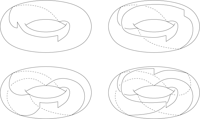
Figure 9. The knots $K(3,5;1)$, $K(3,5;2)$, $K(3,5;3)$, and $K(3,5;4)$. The first two are trivial, $K(3,5;3)$ is a $(2,3)$ torus knot, and $K(3,5;4)$ is a $(2,5)$ torus knot.

Define knots $K(p,q;k)\subset T\times I$ as follows.

Definition 6.2.

In the universal cover $\operatorname{{\mathbb{R}}}^{2}\times I$ of $T\times I$, take the arc (i. e. line segment) from $((0,0),0)$ to $((kp/q,k),0)$. If $k<q$, add to this arc the arc from $((kp/q,k),0)$ to $((kp/q,k),1)$, followed by the arc from $((kp/q,k),1)$ to $((p_{k},k),1)$, followed by the arc from $((p_{k},k),1)$ to $((p_{k},k),0)$. The image of these arcs in $T\times I\subset S^{3}$ is $K(p,q;k)$. In particular, $K(p,q;q)$ is the standard $(p,q)$ torus knot.

Figure 9 shows the knots $K(3,5;1)$, $K(3,5;2)$, $K(3,5;3)$, and $K(3,5;4)$.

The upper tunnel $\tau(p,q;k)$ of $K(p,q;k)$ is best described by a picture, given as Figure 10. In particular, $\tau(p,q;q)$ is the standard upper tunnel of the $(p,q)$ torus knot. Figure 10 shows tunnel arcs for the upper tunnels $\tau(3,5;3)$ and $\tau(3,5;4)$. We will see, inductively, that the unions of such knots with the particular arcs shown in Figure 10 are the $\theta$-curves dual to the disks of the principal vertex of the tunnel.

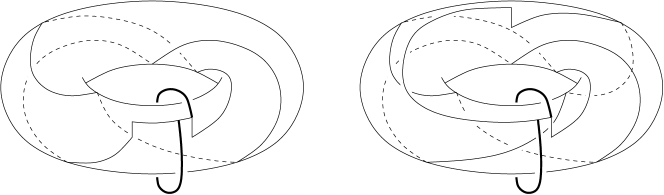
Figure 10. Representative arcs of the tunnels $\tau(3,5;3)$ and $\tau(3,5;4)$.

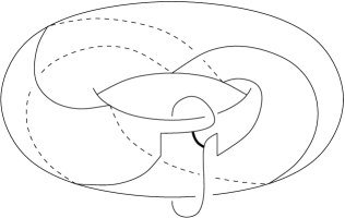
Figure 11. The result of the cabling construction producing $\tau(3,5;4)$ from $\tau(3,5;3)$. After isotopy, this becomes the second drawing in Figure 10.

The cabling construction that takes $\tau(p,q;k)$ to $\tau(p,q;k+1)$ is illustrated in Figure 11 for the case of $\tau(3,5;3)$. The resulting knot is isotopic to the $K(3,5;4)$ shown in Figure 10, by pushing the arc that was the tunnel arc of $\tau(3,5;3)$ down into $T$ and stretching out the new tunnel arc until it looks like the one in Figure 10.

2pt $\lambda^{+}$ [B] at 198 640 $\tau^{+}$ [B] at 187 510 $\rho^{0}$ [B] at 255 548 $\rho$ [B] at 397 735 $\tau^{-}$ [B] at 622 626 $\lambda^{-}$ [B] at 619 512 $\tau^{+}$ [B] at 260 300 $\tau$ [B] at 90 140 $\tau^{-}$ [B] at 255 -27 $\rho^{0}$ [B] at 398 300 $\rho$ [B] at 485 141 $\lambda^{+}$ [B] at 550 300 $\lambda$ [B] at 703 140 $\lambda^{-}$ [B] at 544 -27

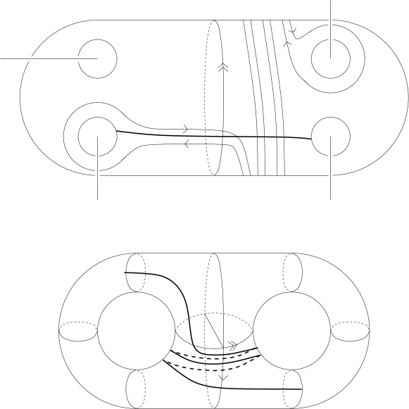
Figure 12. The slope calculation for the cabling taking $\tau(p,q;k)$ to $\tau(p,q,k+1)$. In the top picture, $\rho^{0}$ makes $p_{k}$ turns around the ball; for the example drawn here, $p_{k}=3$. The cabling arc for the new tunnel disk has $2p_{k}-1$ crossings with $\rho^{0}$, producing the slope pair $[1,2p_{k}-1]$ as seen in the standard picture.

We will now compute the slopes of these cabling operations. Figure 12 illustrates the calculation for the cabling taking $\tau=\tau(p,q;k)$ to $\tau(p,q,k+1)$. The ball shown in the top drawing in Figure 12 is a regular neighborhood of the arc in the raised part of $K(p,q;k)$ that connects the endpoints of $\tau(p,q;k)$. The disk $\rho$ will be replaced.

The $0$-slope disk $\rho^{0}$ makes $p_{k}$ turns around the ball. To see this, consider a perpendicular disk $\rho^{\perp}$ for $\rho$ constructed as follows. In the boundary of the ball in Figure 12, take an arc $\alpha$ connecting $\partial\tau^{+}$ to $\partial\tau^{-}$, running across the front of the ball between $\partial\lambda^{+}$ and $\partial\lambda^{-}$, and cutting across $\partial\rho$ in a single point. The frontier of a regular neighborhood of $\tau^{+}\cup\alpha\cup\tau^{-}$ in the ball is $\rho^{\perp}$. That is, $\rho^{\perp}$ is like $\rho^{0}$ except that it has no turns around the back of the ball. The representative of $K_{\tau}$ disjoint from $\rho^{\perp}$ is isotopic to $K(p,q;k)$, while the representative of $K_{\lambda}$ is a core circle of $W$ that completely encircles this $K(p,q;k)$. In the homology of $V\cup T\times I$, $K(p,q;k)$ represents $p_{k}$ times the generator, so (for some choice of linking conventions) $K_{\lambda}$ has linking number $p_{k}$ with $K_{\tau}$. Adding $p_{k}$ turns around the ball to $\rho^{\perp}$ as in the top drawing of Figure 12 decreases this linking number to $0$, and gives the perpendicular disk shown in Figure 12, which must therefore be $\rho^{0}$.

Both diagrams in Figure 12 show the cabling arc for the slope disk that defines $\tau(p,q;k+1)$, and the bottom picture verifies that its slope coordinates are $[1,2p_{k}-1]$. This yields the value for $m_{k}$ given in Theorem 1.2.

We can begin the process with the knot $K(p,q;1)$. For the standard tunnel arc, all three of the disks $\lambda$, $\rho$, and $\tau$ in the first drawing of Figure 12 are primitive, since $K_{\lambda}$, $K_{\rho}$, and $K_{\tau}$ are trivial knots. For $k<k_{0}$, $p_{k}=1$ and $K(p,q;k+1)$ is a trivial knot. This can be seen geometrically, but also follows inductively from the fact that these cablings have simple slope $\Big{[}\displaystyle\frac{1}{2\cdot 1-1}\Big{]}=[0]\in\operatorname{{\mathbb{Q}}}/\operatorname{{\mathbb{Z}}}$. The process terminates with the cabling corresponding to $k=p_{q-1}$, which produces $K(p,q;q)=K_{p,q}$.

7. Applications

Here we will recover the classification of the torus knot tunnels of M. Boileau, M. Rost, and H. Zieschang [2] and Y. Moriah [8], although not their result that these are all the tunnels. We consider three cases for $K_{p,q}$:

Case I. $|p-q|=1$.

We may assume that $(p,q)=(n+1,n)$ with $n\geq 2$. For both the upper and lower tunnels, Theorem 1.2 gives $[1/3]$, $5$, $7,\ldots\,$, $2n-1$ as the slope sequence. For the middle tunnel, Theorem 1.1 gives the same slope sequence, and all $s_{i}=0$, showing that all three tunnels are the same.

Case II. $|p-q|\neq 1$, but $p\equiv\pm 1\mod{q}$ or $q\equiv\pm 1\mod{p}$

Again we assume that $p,q\geq 2$, and reduce to the case when $p>q$. Suppose first that $p=mq+1$ with $m\geq 2$. For the upper tunnel, Theorem 1.2 gives slopes $[1/(2m+1)]$, $4m+1$, $6m+1,\ldots\,$, $2m(q-1)+1$ (to find the $p_{k}$, notice that the line segment in $\operatorname{{\mathbb{R}}}^{2}$ from $(1,0)$ to $(mq+1,q)$ passes through the lattice points $(m+1,1)$, $(2m+1,2)$, $(3m+1,3)$, and so on, then slide the left endpoint from $(1,0)$ to $(0,0)$). This equals the sequence obtained for the middle tunnel using the continued fraction expansion $(mq+1)/q=[m,q]$, and Theorem 1.1 also gives all $s_{i}=0$. For the lower tunnel, the sequence is $[1/3]$, $3,\ldots\,$ $3$, $5,\ldots\,$ $5$, $7,\ldots\,$ $7\,\ldots\,$, $2q-1$, where each value is repeated $m$ times, except that $3$ appears $m-1$ times. Thus the middle tunnel is equivalent to the upper tunnel and distinct from the lower tunnel.

For the case when $p=mq-1$, a similar examination (using the line segment from $(0,0)$ to $(mq,q)$ and sliding the right-hand endpoint to $(mq-1,q)$) finds the slopes to be $[1/(2m-1)]$, $4m-1,\ldots\,$, $2m(q-1)-1$. The continued fraction expansion is $(mq-1)/q=[m-1,1,q-1]$, and the algorithm for the middle tunnel gives the same slope sequence and all $s_{i}=0$. For the lower tunnel, the sequence is $[1/3]$, $3,\ldots\,$ $3$, $5,\ldots\,$ $5$, $7,\ldots\,$ $7\,\ldots\,$, $2q-1$, where each value is repeated $m$ times, except that $3$ and $2q-1$ are repeated $m-1$ times. Again, the middle tunnel is equivalent to the upper tunnel and distinct from the lower tunnel.

Case III. Neither Case I nor Case II

In these cases, Theorem 1.1 shows that the middle tunnel has at least one nonzero value of $s_{i}$, so is distinct from the upper and lower tunnels. Reducing to the case when $p>q\geq 2$, Theorem 1.2 shows that the slopes are all distinct for the upper tunnel, but there is a repeated slope for the lower tunnel. This completes the verification.

We note that the cases when there are fewer than three tunnels are exactly those for which the middle tunnel is semisimple. This verifies the equivalence of the first two conditions in the following proposition. The equivalence of the first and third is from [2].

Proposition 7.1.

For the $(p,q)$ torus knot $K_{p,q}$, the following are equivalent:

1. $p\not\equiv\pm 1\pmod{q}$ and $q\not\equiv\pm 1\pmod{p}$.

2. The middle tunnel is regular.

3. $K_{p,q}$ has exactly three tunnels.

References

- [1] E. Akbas, A presentation of the automorphisms of the -sphere that preserve a genus two Heegaard splitting, Pacific J. Math. 236 (2008), 201-222.
- [2] M. Boileau, M. Rost, and H. Zieschang, On Heegaard decompositions of torus knot exteriors and related Seifert fibre spaces, Math. Ann. 279 (1988), 553–581.
- [3] S. Cho, Homeomorphisms of the -sphere that preserve a genus Heegaard splitting, Proc. Amer. Math. Soc. 136 (2008), 1113–1123.
- [4] S. Cho and D. McCullough, The tree of knot tunnels, to appear in Geom. Topol.
- [5] S. Cho and D. McCullough, Constructing knot tunnels using giant steps, preprint.
- [6] S. Cho and D. McCullough, Tunnel leveling, depth, and bridge numbers, preprint.
- [7] S. Cho and D. McCullough, software available at www.math.ou.edu/dmccullough/ .
- [8] Y. Moriah, Heegaard splittings of Seifert fibered spaces, Invent. Math. 91 (1988), 465–481.
- [9] M. Scharlemann, Automorphisms of the 3-sphere that preserve a genus two Heegaard splitting, Bol. Soc. Mat. Mexicana (3) 10 (2004), 503–514.
- [10] M. Scharlemann and A. Thompson, Unknotting tunnels and Seifert surfaces, Proc. London Math. Soc. (3) 87 (2003), 523–544.