Ascending and descending regions of a discrete Morse function

Abstract

We present an algorithm which produces a decomposition of a regular cellular complex with a discrete Morse function analogous to the Morse-Smale decomposition of a smooth manifold with respect to a smooth Morse function. The advantage of our algorithm compared to similar existing results is that it works, at least theoretically, in any dimension. Practically, there are dimensional restrictions due to the size of cellular complexes of higher dimensions, though. We prove that the algorithm is correct in the sense that it always produces a decomposition into descending and ascending regions of the critical cells in a finite number of steps, and that, after a finite number of subdivisions, all the regions are topological discs. The efficiency of the algorithm is discussed and its performance on several examples is demonstrated.

1 Introduction and motivation

Given a smooth manifold $M$ with a Morse function $F$ defined on it, classical Morse theory [1], [2] is a powerful tool for investigating the behavior of the function $F$, as well as the topological properties of $M$. The critical points of $F$ together with their indices determine a handlebody decomposition of the domain $M$. A different decomposition of $M$, carrying topological as well as geometric information, is obtained from the stable and unstable manifolds of the critical points. The intersections of these are regions where the function behavior is uniform in the sense that all gradient paths have the same asymptotic behavior. If the function is Morse-Smale, that is, if the stable and unstable manifolds of the critical points intersect transversely, then these regions form the Morse-Smale CW-complex. Such a decomposition enables a thorough understanding of the domain $M$, as well as of the gradient flow of the function $F$.

Consider for example the function shown on figure 1. Assume that the function models a geographic terrain, and that our task is to find a path starting at a point $(x,y)$ in the descending disk of one of the maxima and ending in our preferred maximum $(x_{0},y_{0})$, which is traced optimally with respect to some criterion, for example height variation. This can be reconstructed from the descending and ascending disks, but these are computationally expensive. The problem is even more difficult if, instead of the function $f(x,y)$, only a sample of points on the surface is given. What we need, is a discrete approximation of the ascending and descending disks of $F$. Once this is given, the required path can be constructed so that it first reaches a saddle in the common boundary of both maxima, and then ascends towards the preferred one.

Figure 1: A model of a geographical terrain

In this paper we propose an algorithm based on the discrete Morse theory of Forman [3], [4] to solve this problem. Discrete Morse theory is a PL analogue of classical smooth Morse theory which has gained wide popularity and is used in topological data analysis [5], [6], [7], [8] as well as in addressing purely theoretical topological and combinatorial problems, as for example in [9], [10], [11].

In order to use discrete Morse theory for analyzing data, the initial data are first extended to a discrete Morse function on a triangulation (or, more generally, regular cellular decomposition) of the domain. This can be done using for example the algorithm of [12] (which is used in our implementations). The algorithm of this paper provides a further step by constructing the descending and ascending regions of the discrete Morse function and, from these, the discrete Morse-Smale complex.

The construction of discrete descending regions of a critical cell is motivated by the definition of descending disks in the smooth case: as unions of $V$-paths, which are the discrete analogue of gradient paths, starting in the critical cell. Discrete ascending regions are constructed using the same procedure on the dual $V$-paths in the dual complex $K^{*}$. The resulting decomposition into descending regions is similar to the smooth case in top dimension where the obtained regions are disjoint topological disks. In lower dimensions they are not necessarily disjoint, and not always disks, since, unlike gradient paths in the smooth case, $V$-paths from different critical cells or even from the same critical cell ending in the boundary of a specific critical cell $s$ can merge before reaching this boundary. We show, though, that after a finite number of subdivisions such merges can be eliminated, so that, as in the smooth case, the descending regions and the ascending regions form two families of disjoint topological disks. The regions obtained typically do not intersect transversely. This is not a major problem in the discrete case, though. The intersections nevertheless provide a discrete Morse-Smale decomposition of the cells of the domain into regions where, like in the continuous case, all $V$-paths come from and tend towards the same two critical cells.

In [11], Theorem 3.1 the connection between discrete and smooth Morse theory is described in detail. It is shown that a smooth Morse function $F$ on a closed Riemannian manifold $M$ can be approximated by a discrete Morse function $f$ on a $C^{1}$ triangulation of $M$ so that critical points of $F$ correspond to critical cells of $f$. If, in addition, the function $F$ is Morse-Smale, the $V$-paths connecting any pair of critical cells $p$ and $q$ such that $\dim(p)=\dim(q)+1$ are in bijection with integral curves of the gradient vector field of $F$ between the corresponding critical points.

Several other algorithms for constructing discrete ascending and descending disks, as well as a discrete Morse-Smale complex exist. A classical example of an application of such a decomposition is the watershed segmentation algorithm in digital image analysis [13, 14]. In [15] a discrete Morse-Smale decomposition of a surface was constructed and applied to geographic surface modeling, in [16], using a different approach, such a decomposition was used in molecular modelling. In [17] 3D Morse-Smale complexes are used in volumetric data analysis. In [18] an algorithm for constructing a quasi Morse-Smale complex, a combinatorial analogue of a 3D Morse-Smale complex, is given and in [19] an extension of this algorithm is applied to several well known data sets. An overview of computational Morse theory with a large number of additional references and applications can be found in [20]. All existing algorithms are restricted to 2 or 3 independent variables, though, while real-world data often depends on more than 3 variables.

Our algorithm works, theoretically, in any dimension, and we have implementations in OCAML, C++ and C# that accept simplicial or, more generally, polyhedral complexes without dimensional restrictions as input. In practice, however, the implementations can be used for simplicial complexes of dimension 6 or less, since the number of cells in a complex grows exponentially with the dimension, and the complexity of the algorithm depends on the number of cells. One of the applications described in the last section uses a 4-dimensional data set.

An additional advantage of discrete Morse theory, in comparison to other approaches, is an efficient and elegant mechanism for dealing with noise which produces, after canceling pairs of critical cells, a simplified function in the sense that the number of critical elements is reduced. This is similar to handle sliding in computational Morse theory of [18] and [15], and allows the use of persistence [21], [22] which has proven to be extremely useful in topological analysis of data [23], [24], [19].

The paper is organized as follows. In Section 2 we give a short overview of discrete Morse theory and introduce notation. In Section 3 we describe the construction of descending and ascending regions of critical cells, and discuss the complexity and the properties of the resulting decomposition. Finally, Section 4 contains several demonstrations and applications of our algorithm. We first give a short description of an application of our algorithm to qualitative data analysis in artificial intelligence presented in [25]. Next, an analysis of the response of a mechanical system consisting of a cart and a rod attached to its top is described. Our third example concerns the problem, presented in the beginning of this section. A procedure for constructing an optimal path (with respect to some optimization criterion) using the decomposition into descending regions is described, which is well defined also in the case, where the descending and ascending regions are not disks. Finally, we use our decomposition to construct a macroeconomic model on a 4-dimensional data set. This is part of an ongoing project with the goal to find and algorithm for controlling the key parameters of the model which contribute to long term economic growth of a country.

Part of this work was the result of a cooperation with the Laboratory for artificial intelligence at the Faculty of Computer and Information Science, University of Ljubljana. We would like to thank the members of this lab for the permission to use data gathered in their experiments. Our thanks also go to the anonymous referees for valuable comments which have helped to improve this paper.

2 Discrete Morse theory

A discrete Morse function on a regular cellular complex $K$ associates to every cell $\sigma\in K$ a real number $f(\sigma)$ such that in most cases $f$ increases with increasing dimension except, possibly, in one direction. More precisely, for every cell $\tau^{(p)}\in K$ of dimension $p$ the number of its codimension 1 faces with values of $f$ greater than $f(\sigma)$ is at most one, and also the number of its codimension 1 cofaces with values of $f$ smaller than $f(\sigma)$ is at most $1$. That is:

$$b(\tau)=\#\{\nu^{(p-1)}\,|\,\nu<\tau,f(\nu)\geq f(\tau)\}\leq 1$$

$$a(\tau)=\#\{\sigma^{(p+1)}\,|\,\tau<\sigma,f(\tau)\geq f(\sigma)\}\leq 1.$$

The numbers $a(\tau)$ and $b(\tau)$ can not both be one. Since, if there exists a face $\nu<\tau$ such that $f(\nu)\geq f(\tau)$ as well as a coface $\sigma>\tau$ such that $f(\sigma)<f(\tau)$, then for any $\tau^{\prime}<\sigma$ such that $\nu<\tau^{\prime}$, as in figure 2 (where the arrows indicate the direction of function descent) it follows that

$$f(\tau^{\prime})>f(\nu)\geq f(\tau)\geq f(\sigma)>f(\tau^{\prime})$$

which is a contradiction.

Figure 2: A discrete Morse function can not have both $a(\tau)$ and $b(\tau)$ equal to $1$

Because of this, the cells of $K$ split into three subsets $K=A\cup B\cup C$ (in the terminology of [12]). If both $a(\tau)=b(\tau)=0$ then $\tau$ is a critical cell of index $p=\dim\tau$, and $C$ is the set of all critical cells. If not, either $a(\tau)=1$ or $b(\tau)=1$, and $\tau$ is a regular cell. A regular cell $\tau$ belongs to the set $A$ if $a(\tau)=1$ and to $B$ if $b(\tau)=1$.

For each $\tau\in A$ there exists precisely one $\sigma\in B$ such that $\tau<\sigma$ and $f(\tau)\geq f(\sigma)$. The map $V:\ A\to B$ which associates $\tau^{(p)}$ to $\sigma^{(p+1)}$ is called a discrete gradient vector field, and points in the direction of steepest descent from the cell $\tau$.

It is convenient to imagine a discrete gradient vector field not as a map but as a collection of pairs $(\tau^{(p)},\sigma^{(p+1)})$ such that $V(\tau)=\sigma$, or arrows from $\tau$ to $\sigma$, in the direction of function descent. This representation of a discrete gradient vector field is used in all figures in this paper. The cells of $K$ which are unpaired are precisely the critical cells.

In classical Morse theory the gradient vector field points in the direction of steepest ascent of the function $f$, and its gradient paths (traced in the direction opposite to the gradient flow) are the paths of steepest descent. The discrete analogue is a $V$-path, which is a sequence of cells

$$\tau_{0}^{(p)}<\sigma_{0}^{(p+1)}>\tau_{1}^{(p)}<\sigma_{1}^{(p+1)}...\tau_{r}^{(p)}<\sigma_{r}^{(p+1)}>\tau_{r+1}^{(p)}$$

such that $V(\tau_{i})=\sigma_{i}$ and $\tau_{i+1}$ is a face of $\sigma_{i}$ different from $\tau_{i}$ for $i\in\{1,..,r\}$.

As in the classical case, function values decrease along a $V$-path. This implies that a $V$-path of a discrete gradient vector field $V$ arising from a discrete Morse function can not be closed, that is, the discrete gradient vector field can not contain any cycles. Forman showed that this is characteristic for discrete gradient vector fields: a pairing $V$ arises from a discrete gradient vector field of a discrete Morse function on $K$ if and only if it contains no nontrivial closed $V$-paths.

In classical Morse theory, two critical points $p_{1}$ and $p_{2}$ of a Morse function $F$ on $M$ of indices differing by $1$ can be canceled when there exists exactly one gradient path between them. That is, using handle sliding, $F$ can be smoothly deformed to a function $F^{\prime}$ which has exactly the same critical points as $F$ except $p_{1}$ and $p_{2}$ that become regular. This is true also in the discrete case. If the critical cells $\sigma$ and $\tau$ are connected by exactly one $V$-path starting in any cell of $\partial\sigma$ and ending in $\tau$, i.e.

$$\sigma^{(p+1)}=\sigma_{-1}^{(p+1)}>\tau_{0}^{(p)}<\sigma_{0}^{(p+1)}>\tau_{1}^{(p)}<\sigma_{1}^{(p+1)}\ldots\tau_{r}^{(p)}<\sigma_{r}^{(p+1)}>\tau_{r+1}^{(p)}=\tau^{(p)}$$

then the pair $\sigma,\tau$ can be cancelled. This is done simply by modifying the discrete gradient vector field $V$ along the connecting paths to

$$V^{\prime}(\tau_{i})=\sigma_{i-1}$$

for $i\in{0,...,r+1}$. This procedure can also be described as switching the direction of the arrows along the connecting $V$-path. Since there are no other $V$-paths connecting $\tau_{0}^{(p)}<\partial\sigma$ and $\tau^{(p)}$ this can not create a non-trivial closed $V^{\prime}$-path and so, according to Forman’s characterization, the modified $V^{\prime}$ is the discrete gradient vector field of some Morse function for which the cells $\tau$ and $\sigma$ are no longer critical.

3 Algorithm

In this section we present our algorithm which, on the basis of a discrete Morse function $f$, produces two decompositions of a regular cellular complex $K$ with $|K|$ a manifold. First, a decomposition of $K$ into discrete descending regions of the critical cells of $f$ is constructed. Each of the regions contains exactly one critical cell $s^{(p)}$, the maximum of the region, and a collection of regular cells of dimension less than or equal to $p$.

In the second step we decompose, using the same procedure, the dual complex $K^{*}$ into discrete descending regions of the function $-f$. This gives a decomposition of $K$ into discrete ascending regions of the critical cells.

3.1 Constructing the descending regions

In the smooth case, the unstable manifold of a critical point $c$ of $F$ is the union of all gradient paths of the flow $-$grad $F$ starting close to the point $c$. In the discrete case the direction of function descent is indicated by the discrete gradient vector field $V$, which plays a similar role as the gradient vector field in the smooth case. The discrete descending region $D(s^{(p)})$ of a critical cell $s^{(p)}$ thus contains all regular cells which appear in a $V$-path starting in the boundary of $s^{(p)}$. The descending region is constructed in two steps. In the first step the frame which contains all cells of maximal dimension is constructed, and in the second step the cells of lower dimension are added.

The critical cells are first ordered by ascending dimension so that, when processing a critical cell of dimension $d$, the descending regions of all critical cells of dimension less than $d$ have already been constructed. This will be very important in the second step of the algorithm.

Let $s^{(p)}$ be a critical cell. The frame $\texttt{fr}(s)$ consists of all regular $p$ and $(p-1)$ dimensional cells appearing in a $V$-path starting in the boundary of $s$. This part of the algorithm is a simple breadth-first search through the regular $(p-1)$-faces of the included $p$-cells which terminates when no more regular $(p-1)$-cells belonging to the set $A$ (that is, no more $(p-1)$-dimensional arrow tails) can be found. Since a cell in the frame can typically be reached by several paths in $V$, a set structure is used for storing the cells to eliminate duplicates.

This step of the algorithm is illustrated in figure 3. On the left, the discrete gradient vector field is shown, the descending frame of the maximum is in the middle and the descending frame of the saddle is on the right.

Figure 3: Building the frame of descending regions in a cellular complex

The frame $\texttt{fr}(s^{(p)})$ contains only $p$ and $p-1$ dimensional cells. The next step is to decide which additional faces of the cells in $\texttt{fr}(s)$ should be included.

Consider a $V$-pair $(\alpha,\beta)$ incident to some simplex from $\texttt{fr}(s^{(p)})$. Since $V(\alpha)=\beta$, function values decrease from $\alpha$ towards $\beta$. This implies that $\beta$ belongs to the descending region $D(s)$ when $\alpha$ does, so the pair $(\alpha,\beta)$ is included into or excluded from the descending region together. It is included if all codimension one cofaces of $\alpha$ except $\beta$ have already been included. This is implemented by the following recursively used routine. Let $S$ be the set of all $(p+1)$-dimensional cofaces of $\alpha$, different from $\beta$, and incident to some $p$-dimensional cell from $\texttt{fr}(s)$. The routine checks if all elements of $S$ belong to $D(s)$. It ends when either a cell $\gamma^{(d+1)}\in S$ is found that belongs to the descending region of some other critical cell of dimension less than $p$, in this case the pair ($\alpha$,$\beta$) is not included, or all cells of $S$ have been included in $D(s)$, and in this case the pair $(\alpha,\beta)$ is also included.

On figure 4 the left picture again shows the discrete gradient vector field. In the middle picture, part of the descending region of the maximum is already constructed (the 2-cells forming the frame are shaded, and the 1-cells that are already included are bold), and the pair $(\alpha,\beta)$ that is processed is the diamond-shaped point and the dashed edge. Since all edges that have this point as a face are already included in the descending disk, the pair $(\alpha,\beta)$ is added. On the right, the situation is different. The descending disk of the saddle has already been constructed and contains the dashed edge $\beta$. Since $\beta$ already belongs to the descending region of the saddle, the pair $(\alpha,\beta)$ will not be included.

Figure 4: Completing the descending region

Proposition 1

The construction of the descending region of a critical cell ends in a finite number of steps.

[Proof] During frame construction we simply follow the direction of the discrete gradient vector field $V$. Since $V$ does not contain nontrivial closed paths and the complex $K$ is finite the frame is completed in a finite number of steps.

The second step of the construction, where lower dimensional cells are added, is recursive. The algorithm runs through all $V$-pairs in the boundary of frame cells. For each pair $(\alpha^{(d)},\beta^{(d+1)})$ which has not been processed it checks if all cofaces of $\alpha$ of dimension $(d+1)$ are already included in the descending region. If it encounters a coface which has not been processed it checks that first. This implies that the algorithm always proceeds in the direction opposite to $V$, so no cycles can be created.

Since the number of pairs is finite, the algorithm ends in a finite number of steps. Notice that the algorithm can start processing pairs in any order, independent of dimension.

3.2 The boundary

The algorithm described in the previous section constructs discrete descending regions of a discrete Morse function on a complex $K$ with $|K|$ a manifold without boundary. For manifolds with boundary, the boundary must be processed separately.

Denote the discrete gradient vector field of the restriction of $f$ to the boundary by $V_{\partial K}$. A critical cell $\nu$ of $V_{\partial K}$ is

1. either a critical cell in $V$

2. or is paired to a higher dimensional cell that does not belong to the $\partial K$; such cells will be called boundary critical cells.

In the first case no extra processing is needed, as $\nu$ is also a critical cell in $V$ and its descending region has been constructed in the previous step.

In the second case, the discrete descending region of a boundary critical cell $\nu^{(p)}$ is constructed in two stages. First, the discrete descending region of the critical cell $\nu^{(p)}$ in $\partial K$ is found using the algorithm of the previous section. In the second stage, all cells of dimension $p$ in the discrete descending region of $\nu^{(p)}$ in $\partial K$, that are paired by $V$ to a higher dimensional cell $\beta$ in the interior, are considered. The cell $\beta$ is processed as a critical cell and its descending region is constructed. The union of all regions obtained in this way constitutes the descending region of the boundary critical cell $\nu$.

For example, consider $f(x,y)=x+y$ on a triangulation of the square $[0,1]\times[0,1]$. The discrete gradient vector field contains all cells except a minimum on the boundary which is the only critical cell

Figure 5: Discrete gradient vector field on the square and its boundary

The discrete gradient vector fields of $f$ and $f|_{\partial K}$ are shown on Figure 5. The maximum $\mu$ of $f|_{\partial K}$ is a boundary critical $1$-cell. Its descending region in $\partial K$ is all of $\partial K$ except for the minimum. A boundary cell $\alpha$ which is paired with an interior cell $\beta$ in $V$ is included into the descending region of $\mu$ together with $\beta$ and its descending region. Finally, the descending region of $\mu$ is the entire square without the minimum.

3.3 Ascending regions

The ascending regions of the critical cells of $f$ on $K$ are obtained from the dual complex $K^{*}$ with the dual the discrete gradient vector field $V^{*}$.

Viewing $K$ as an abstract regular cell complex determined by its cells with specified dimension and the face relationship between them, the dual complex $K^{*}$ is obtained simply by reversing the dimensions and the face relationship on the cells. That is, a cell $\alpha^{(p)}\in K$ corresponds to a cell $\alpha^{*(n-p)}\in K^{*}$, where $n$ is the dimension of $K$, and if $\alpha$ is a face of $\beta$ in $K$, then $\alpha^{*}$ contains $\beta^{*}$ as its face in $K^{*}$. In the geometric realization $|K|$ of $K$, the vertices of $K^{*}$ correspond to barycenters of the $n$-cells of $K$, while a cell of higher dimension is spanned by a collection of vertices of $K^{*}$ such that the corresponding $n$-cells of $K$ have a nonempty intersection. If $|K|$ is a PL-manifold without boundary, then $|K^{*}|=|K|$. If $|K|$ is a PL-manifold with boundary, then $K^{*}$ is not a cell decomposition of $|K|$ any more, since the cells of $K^{*}$ which are dual to boundary cells of $K$ do not have a sufficient number of faces (for example, a $1$-cell of this type has only $1$ face). For our purpose $K^{*}$ is just a combinatorial object, though, so this geometric property does not represent a problem.

Also the dual discrete vector field $V^{*}$ is obtained simply by reversing the arrows in $V$. That is, two cells $\alpha^{*}$ and $\beta^{*}$ are paired in $V^{*}$ if the cells $\beta$ and $\alpha$ are paired in the original discrete gradient vector field $V$. Thus, a cell $\alpha$ in $K$ is critical of index $p$ if and only of the cell $\alpha^{*}$ is critical of index $(n-p)$ in $K^{*}$.

The discrete ascending region of a critical cell $\alpha$ of $K$ is the dual of the discrete descending region of the critical cell $\alpha^{*}$ of $K^{*}$ (see figure 6).

Figure 6: Ascending region of a saddle

3.4 Consistency

The descending and ascending disks of a smooth Morse function $f$ on a manifold $M$ form a decomposition of $M$ into topological disks. If the function is Morse-Smale, their intersections form the Morse-Smale complex on $M$. In the discrete case, the descending and ascending regions obtained are always disks only in the top dimension, while in lower dimensions they might not be disks. In addition, they might not be disjoint, that is, a cell can belong to the descending or ascending disk of more than one critical cell. We first prove that the descending regions (and therefore also the ascending regions) of all critical cells form a covering of the underlying PL manifold.

Proposition 2

Let $K$ be a regular $n$-dimensional cellular complex such that $|K|$ is a manifold without boundary and let $V$ be the discrete gradient vector field of a discrete Morse function on $K$. Then every regular cell $\alpha\in K$ is contained in the discrete descending region of a critical cell $\beta$.

This is true also for manifolds with boundary, if the discrete gradient vector field of $f$ on $K$ is an extension of a discrete gradient vector field of $f\mid_{\partial K}$.

[Proof] We first prove that every regular top dimensional cell $\alpha^{(n)}$ is included in the frame of some top dimensional critical cell. A regular cell of top dimension is paired either to a cell $\gamma_{0}^{(n-1)}$ which is a face of at least one $n$-dimensional cell $\alpha_{1}$ other than $\alpha_{0}$, or it is paired to a boundary critical cell $\nu^{(n-1)}$ of top dimension in $\partial K$. In the second case, $\alpha^{(n)}$ belongs to the descending disk of $\nu^{(n-1)}$. In the first case, if $\alpha_{1}$ is critical, then $\alpha_{0}$ lies in its descending region, and if it is regular, we repeat the same process for $\alpha_{1}$. Since the discrete gradient vector field $V$ does not have cycles and $K$ is a finite cellular complex this process must end in a finite number of steps at a critical cell $\alpha_{i}^{(n)}$ or a boundary critical cell, and $\alpha_{0}$ belongs to its descending disk.

Assume now that descending disks of all critical cells have been built and that there exists a regular pair $(\alpha^{(p)},\beta^{(p+1)})$ that is not included in any of them.

Since every cell is a face of some top-dimensional cell, $\alpha$ was processed during the construction of the descending region of some cell $\sigma$. Since it was not included, there exists a coface $\gamma_{1}^{(p+1)}$ of $\alpha$, such that $\gamma_{1}$ is included in the descending region $D(\sigma_{1}^{(n_{1})})$, where $n_{1}<n$. In the construction of the descending region $D(\sigma_{1}^{(n_{1})})$ also $\alpha$ was processed since it is also a face of $\gamma_{0}$, and not included. So there must exist a coface $\gamma_{2}^{(p+1)}$ of $\alpha$ which belongs to some other descending region $D(\sigma_{2}^{(n_{2})})$, where $n_{2}<n_{1}$. This argument can be repeated indefinitely, and we obtain an infinite sequence of critical cells $\sigma_{0},\sigma_{1},\sigma_{2}\ldots$ with strictly decreasing positive dimensions which is a contradiction. So every regular pair $(\alpha^{(p)},\beta^{(p+1)})$ is included in the descending region of some critical cell.

In smooth Morse theory the stable and unstable manifolds of a critical point are constructed from gradient paths, that is, integral curves of the gradient vector field, which begin or end at this point, respectively. An important property of integral curves of a smooth vector field is that they are pairwise disjoint - two different integral curves can be arbitrarily close but do not merge. The discrete analogue of a gradient path is a $V$-path, and since there is no such thing as ‘arbitrarily close’ in the discrete world, a $V$-path typically splits into multiple paths, and several $V$-paths can merge into one path. Due to this, discrete descending and ascending regions of different critical cells might not be disjoint, since $V$-paths beginning in different critical cells might merge. They also might not be topological disks, except in the highest dimension.

Proposition 3

The descending region of a critical cell of maximal dimension (i.e. a maximum) collapses to the maximal cell. The same is true for ascending regions of a critical cell of dimension $0$ (i.e. a minimum).

[Proof] For every cell $\sigma$ of maximal dimension, its pair is a cell of codimension $1$ which is either a boundary critical cell or it is the face of precisely one other cell of maximal dimension. Because of this there exists precisely one $V$-path starting at some (possibly boundary) critical cell $s$ of maximal index (i.e. a maximum) leading to $\sigma$. Since a discrete vector field has no cycles, every such $V$-path leading to a cell in the boundary of the descending region of $s$ determines a sequence of elementary collapses starting in the boundary of the descending region and ending in $s$. A finite number of such $V$-paths determines the necessary elementary collapses required to collapse the whole descending region to the cell $s$.

For descending regions of critical cells of index smaller than maximal, i.e. saddles, this is not necessarily true, since $V$-paths not containing cells of maximal dimension can merge. Figure 7 shows a section of a 3-dimensional cubical complex where $V$-paths in the descending region of a saddle split and merge again, so that the union is not a disk.

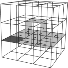
Figure 7: Discrete descending region of a $2$-saddle with splitting and merging $V$-paths

It is possible, however, to modify the decomposition of the cellular complex and the discrete gradient vector field so that the merging point of descending paths is pushed further towards the boundary of the descending region, while the discrete vector field outside the open star of the merging point is left unaffected. The idea is similar to splitting multiple saddles in [15].

The left example on figure 8 shows a section of a 2-dimensional simplicial complex where the descending region of a critical cell of index $1$ is topologically a 1-sphere. The right side of this figure shows the modification which pushes the merging point further along descending values of $f$. The figure shows only one step of the pushing procedure, which can be applied as many times as necessary.

Here is a description of the required modification of a regular cellular complex in the general case. Assume that two $V$-paths

$$\ldots\tau_{i-1}^{(p-1)}<\sigma_{i-1}^{(p)}>\tau_{i}^{(p-1)}=\tau<\sigma^{(p)}>\tau_{i+1}^{(p-1)},\ldots$$

$$\ldots\tau^{\prime(p-1)}_{j-1}<\sigma^{\prime(p)}_{j-1}>\tau^{\prime(p-1)}_{j}=\tau<\sigma^{(p)}>\tau^{\prime(p-1)}_{j+1},\ldots$$

merge in the cell $\tau^{(p-1)}$ which is paired with $\sigma^{(p)}$. Let $S$ be $\texttt{star}(\tau)$ and let $p_{1}$ and $p_{2}$ be two disjoint paths in $S$ from the cell $\sigma_{i-1}$ to the cells $\sigma$ and $\sigma^{\prime}_{j-1}$ respectively.

The required modification consists of replacing $\tau^{(p-1)}$ by two parallel copies $\tau^{(p-1)}$ and $\tau^{\prime(p-1)}$, and $\sigma^{(p)}$ by two copies $\sigma^{(p)}$ and $\sigma^{\prime(p)}$ with $\partial\sigma^{\prime}$ containing the same cells as $\partial\sigma$, except for $\tau$ which is replaced by $\tau^{\prime}$. In addition, two new cells are added: a cell $\nu^{(p)}$ which has cells $\tau^{(p-1)}$ and $\tau^{\prime(p-1)}$ in its boundary, and a cell $\mu^{(p+1)}$ with $\nu,\sigma$ and $\sigma^{\prime}$ in its boundary. We modify the star $S$ in the following way

• in the boundary of all $p$-cells in the path $p_{1}$ (except $\sigma$) the cell $\tau$ is replaced by $\tau^{\prime}$,

• in the boundary of the last $(p+1)$-cell in the path $p_{1}$ $\sigma$ is replaced by $\sigma^{\prime}$,

• $\nu$ is added to the boundary of the first $(p+1)$-cell in the path $p_{2}$,

• $\tau^{\prime}$ and $\nu$ are added to the boundary of all other cells in $S$.

The modified field $V^{\prime}$ coincides with $V$ on both copies of $\tau$, $\sigma$ and their boundaries, and it pairs $\nu$ with $\mu$. The new field $V^{\prime}$ now has two $V^{\prime}$-paths, which possibly merge in some cell $\tau_{i+k}=\tau^{\prime}_{j+l}$ (or are disjoint). So we have pushed the merging point further along the discrete gradient vector field $V$. Also note that this step does not affect $V$-paths originating from critical cells in dimension $p-1$ or lower and does not create any additional merge points for critical paths originating from critical cells of dimension $p$.

Proposition 4

Let $K$ be a finite cellular complex without boundary and let $V$ be a discrete gradient vector field on $K$. Then there exists a finite sequence of steps described above which modify $K$ into $K^{\prime}$ and $V$ into $V^{\prime}$ in such a way that the set of critical cells remains unchanged, and that the descending regions of all critical cells with respect to $V^{\prime}$ are topological disks.

[Proof] The proof goes by ascending dimension of the cells of the complex. Since there is nothing to do for $0$-dimensional critical cells, we start with critical cells of dimension $1$. Let $\tau_{1}^{(0)}$ be the cell where $V$-paths originating from a critical $1$-cell $s$ merge and let $D$ be the descending region of $s$. Since $K$ is finite, a finite sequence of steps described above pushes the cell $\tau_{1}^{(0)}$ into the boundary of $D$. We repeat this process for all such merges in the descending region of $s$. Let $K^{\prime\prime}$ be the resulting complex, $V^{\prime\prime}$ the resulting gradient vector field and $D^{\prime\prime}$ the discrete descending region of $s$ in $K^{\prime}$. Since $D^{\prime\prime}$ does not contain its boundary, and since all merging points have been pushed into the boundary we have pushed the cells where $V^{\prime\prime}$-paths originating from $s$ merge away from $D^{\prime\prime}$. Now the same argument as in the proposition 3 can be used to show that $D^{\prime\prime}$ collapses to the critical cell $s$ and is therefore a topological disk. Also, all $V$-paths coming from critical cells different from $s$ have been pushed off $D^{\prime\prime}$, so $D^{\prime\prime}$ does not intersect any other descending regions.

Since all modifications take place in the interior of the descending disk of $s$, all other descending regions remain unchanged. And since no additional merge points have been created in the process it follows that, after repeating this procedure for all critical $1$-cells, all descending regions originating from critical cells of dimension one are topological disks.

Precisely the same arguments work for critical cells of higher dimension. Assuming that descending regions for critical cells of dimension less than $p$ have already been processed and are therefore topological disks, the descending regions for each critical cells of dimension $p$ is processed in the same way as above. Since all merging points are pushed to the boundary and since no other descending regions are affected, all descending regions of critical cells of dimension $p$ are transformed one by one into disks. Moreover, since the pushing step does not affect the descending regions of critical cells of dimension less than $p$, descending regions of all critical cells of dimension up to $p$ are now topological disks.

Figure 8: One step of pushing a merging point towards the boundary

3.5 Complexity

Let $m$ be the total number of cells of $K$, $n$ the dimension of the complex $K$, $m_{d}$ the number of cells of dimension $d$, $r_{d}$ the average number of codimension $1$ faces (if $K$ is a simplicial complex $r_{d}=d+1)$, $p_{d}$ the average number of codimension $1$ cofaces and $p_{\max}=\max(p_{0},p_{1},\ldots,p_{n})$. Let $c_{t}$ be the total number of critical cells of the discrete Morse function $f$ on $K$, and $c_{d}$ the number of critical cells of dimension $d$.

The frame of a $d$-dimensional critical cell $s^{(d)}$ consists of $d$ and $(d-1)$-dimensional cells that belong to $V$-paths starting in the boundary of $s$. For each $d$-dimensional cell in the frame, the set of its $(d-1)$-dimensional faces has to be found, and for each face its pair in $V$ has to be found. Since faces and their pairs can be found in constant time, this takes at most $\alpha\times r_{d}\times m_{d}$ operations for a suitable constant $\alpha$.

Building all frames of critical cells thus takes $\sum_{i=1}^{n}\alpha\times m_{i}\times r_{i}$ operations. In the case of simplicial complexes, the number of operations is at most $(n+1)\times\alpha\times m\times n$. The complexity of this step is therefore $O(n^{2}\times m)$.

To complete the descending regions requires determining whether a regular cell $q$ that is incident to the region of some descending disk is included in this region. First, its V-pair $p$ has to be found which can be done in constant time. Next, a list of all co-faces of the lower dimensional cell of the pair is required which can also be found in constant time. Each cell in this list is then processed in the same manner. On average it takes $p_{j}$ operations for each cell of dimension $j$, so we need at most $\sum_{i=1}^{d}\alpha^{\prime\prime}\times p_{i}\times m_{i}$ operations to complete the descending region of one critical cell of dimension $d$, where $\alpha^{\prime\prime}$ is a constant. Since we can not use previous results when completing frames for other critical cells some cells are typically checked more than once. So completing a frame for all critical cells takes at most $c_{t}\sum_{i=1}^{d}\alpha^{\prime\prime}\times p_{\max}\times m=c_{t}\times p_{\max}\times m\times n$ operations.

For simplicial complexes the complexity of the algorithm is altogether $O(nm\times(n+c_{t}p_{\max}))$. Note that the algorithm complexity increases exponentially with the dimension of the complex, since the number of cells grows exponentially. In the special case where $K$ is the Delaunay triangulation on a set of points in $\mathbb{R}^{n}$, an upper bound for the total number of cells is $O(v^{\lceil n/2\rceil})$ where $v$ is the number of points. In this case the algorithm has complexity $O(v^{\lceil n/2\rceil}n\times(n+c_{t}p_{\max}))$.

4 Examples

The algorithm presented in this paper has been applied to data sets from different domains. In this section we present some of them.

4.1 The $QING$ algorithm

We first mention the algorithm $QING$ which is an application of our algorithm to AI from [25]. The algorithm uses discrete Morse theory to reconstruct the critical cells of a discrete Morse function obtained from the values of a sampled function. The descending disks obtained using an early implementation of this algorithm were used for the construction of a qualitative graph, that is, an undirected graph $G=(V_{G},E_{G})$ that represents connections between the critical cells. The set of vertices $V_{G}$ is the set of all critical cells. Two points $\alpha$ and $\beta$ from $V_{G}$ with dim $\alpha\geq$ dim $\beta$ are connected if, $\beta$ is in the boundary of the descending region of $\alpha$. This graph was then used in learning in a qualitative model.

The $QING$ algorithm, together with the parametric discrete Morse theory of [6] was used in a learning scheme presented in [26] designed to teach a robot the concept of occlusion.

4.2 Mechanical system response

Our next example is obtained from a model constructed for the purpose of qualitative modeling of data in artificial intelligence. The model is taken from [27]. We would like to thank the authors for permission to use the data. The data represents measurements obtained from a system consisting of a cart and a rod attached to its top in such a way that it can fall either backwards or forwards. The cart is set on ice (or other low-friction surface) and the rod is positioned upwards. As the rod begins to fall, the cart responds, accelerating in the opposite direction of the fall.

Our discrete Morse function models the response of the cart in terms of the acceleration $\ddot{x}$, depending on the rod angle $\varphi$ and the angular velocity $\dot{\varphi}$. The measured values of $\ddot{x}$ are given on a square grid. A discrete gradient vector field was first constructed on a triangulation of the grid using the algorithm of [12] producing, after cancellation, three maxima, four saddles and two minima.

On figure 9 the discrete descending regions of all three maxima are on the left, and discrete descending regions of the four saddles are on the right. The descending regions form a decomposition of the triangulated area into disjoint discs. Note that the critical cell on the right side of the image is a boundary saddle. Its descending area is correctly generated and separates the descending regions of the two maxima.

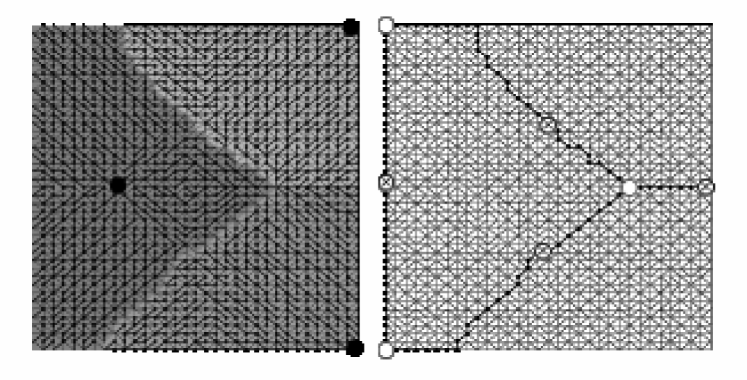
Figure 9: Discrete descending regions of maxima and saddles of the cart function

The exact equation describing this model is

$$\ddot{x}=\frac{a\dot{\varphi}^{2}\sin(\varphi)-b\sin(2\varphi)}{c-d\cos^{2}\varphi}.$$ (1)

Figure 10 shows the graph of this function (with suitable values of $a$, $b$, $c$ and $d$) with the descending discs mapped onto it.

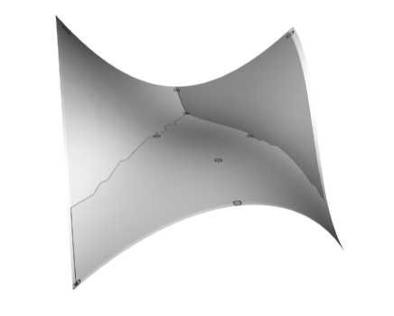
Figure 10: Graph of the cart function with a decomposition into descending disks

The motivation for this example comes from qualitative modeling and simulation in artificial intelligence [28], as a step further after the algorithm $QING$. The idea is, that understanding the response of the cart can provide an optimal strategy for controlling the system in the unstable equilibrium. Given a state of the system described by values of $\varphi$ and $\dot{\varphi}$, a $V$-path from the given state towards this point encodes a strategy for control. Depending on some optimization criterion, an optimal strategy can be chosen. In the next example we give a brief explanation of a controlling strategy towards a maximum.

4.3 Optimal path construction

In this example, a discrete approximation of the Morse-Smale decomposition of the smooth function on figure 1 is first constructed. The function is sampled on a random set consisting of $10^{6}$ points in the domain. The Delaunay triangulation on these points consists of approximately $4*10^{6}$ simplices. A discrete Morse function on this triangulation is constructed. The discrete Morse-Smale complex is shown on figure 11. The required time to build the Morse-Smale complex on a PC was a few seconds. The construction of the discrete Morse function was computationally the most expensive and required (on a laptop) approximately 10 minutes.

We also present a procedure for designing an optimal path, with respect to an optimization criterion involving height variation, from a given a point $A=(x,y)$ in the domain, ending at a preferred maximal cell $\beta$ (for example at the highest one). A slight modification of the described procedure can be used for constructing a path towards any critical point or even towards any point in the domain. Note that the procedure described can be applied in any dimension and can be therefore used to solve similar control problems in a more general setting. Also note, that the path constructed does not have the smallest possible height variation. Such a path would involve the construction of level curves which is not the object of this paper.

Assuming that a triangulation of the domain, a discrete Morse function on it, and a discrete Morse-Smale decomposition are given, we first determine the set of critical cells $S$ with the property, that $A$ lies in their descending regions. Since every cell is contained in at least one descending region, the set $S$ is nonempty, and because $A$ may belong to several descending regions, the set $S$ may contain more than one element.

Let $\alpha$ be a cell of the same dimension as $\beta$ with $a\in\alpha$. If $\beta\in S$ then $\alpha$ is a cell of maximal dimension in the descending disk of $\beta$, so there exists a unique $V$-path from $\beta$ to $\alpha$, and we simply climb up from $\alpha$ along this path.

If $\beta\notin S$, we construct the qualitative graph, as in paragraph 4.1. The next step is to search through paths in the graph $G$ starting from any point $\gamma\in S$ and ending in the required destination $\beta$ to find the path $s$ which minimizes height variation. Note that any other criterion can be used to choose the optimal path at this step.

The required optimal path consists of two parts. The first part connects $\alpha$ with the closest saddle $\gamma$ of index less than $\beta$ in $s$ which lies in the boundary of the descending region of the initial point of $s$. The second part of the path follows $s$ from $\gamma$ to $\beta$.

The cell $\alpha$ is connected to $\gamma$ in the following way. First, all $V$-paths from $\alpha$ are constructed. If any one of them intersects the ascending or descending disk of $\gamma$, we follow this path to the boundary, and then ascend or descend to $\gamma$. If none of them do, we make a step along the unique $V$-path from the initial point of $s$ to $\alpha$, and repeat the procedure. After finitely many steps we either reach the descending or ascending region of the initial point of $s$, or $\alpha$, from where a $V$-path to this point exists.

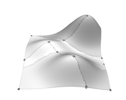
Figure 11: 3D image of the terrain function on figure 1

4.4 A macroeconomic model

In our last application, macroeconomic financial indicators of European countries are analyzed. The data was retrieved from the publicly available database Eurostat [29]. This example is part of an ongoing project involving a qualitative analysis of the effect of key macroeconomic indicators on long term economic growth of a country. The motivation for this project is the hypothesis formulated in [30] that long term economic growth can be achieved by balancing key macroeconomic factors. In this example a five-year average of real GDP (gross domestic product) growth rate $(Ggr)$ is used as a measure of long term economic growth, and the effect of the following macroeconomic indicators as independent variables is analyzed: inflation rate ($I$), balance of current account ($BCA$), and public debt ($PD$). An additional independent variable, GDP per capita ($Gpp$), was used as a control variable to distinguish between different levels of economic development in the countries.

Each point in our model thus represents a point in $\mathbb{R}^{4}$ with coordinates the values of $I$, $BCA$ and $PD$ for one of the European countries in a given year from 1998 to 2004, and the average value of $Gpp$ over this and the next four years. The average value of $Ggr$ over this and the next four years is the dependent variable. Altogether 143 data points representing the countries included in different years were available.

A Delaunay triangulation on the points in $\mathbb{R}^{4}$ was constructed, producing altogether 17451 simplices of dimension up to 4. The discrete vector field was reconstructed from the data points using the algorithm of [12] producing 2 critical cells in dimension 4 (maxima), 13 in dimension 3, 24 in dimension 2, 16 in dimension 1 and 4 critical cells in dimension 0. On a laptop, the descending and ascending disks are reconstructed immediately, once the triangulation and the discrete vector field are given. The reconstruction of the triangulation is also almost immediate, and the discrete gradient vector field is built in less than a minute. The graph, connecting the critical cells with respect to incidence in the boundaries of the corresponding descending regions is given in figure 12.

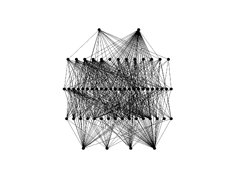
Figure 12: The qualitative graph connecting the critical cells in the 4-dimensional macroeconomic data set.

For each country, data for the current year determines a point in the domain, and the model can be used to predict its average economic growth in the next five years. The $V$-paths encode the changes in the parameter values which ensure constant growth of the GDP growth rate. Finally, the Morse-Smale decomposition can be used to construct a path, similar to the one in example 4.3, which ends in a preferred position involving minimal variation in the GDP growth.

The two maxima correspond to Ireland in 1999 ($m_{1}$) and Latvia in 2003 ($m_{2}$). According expert knowledge from economics, $m_{1}$ represents the preferred maximum (since the high growth in Latvia is partly due to its post transition stage from a state planned economy, and involves high risks in the form of very high inflation, public debt and unemployment). So, for a country which is currently in the descending disc of $m_{2}$ (for example Slovenia), a path leading from its current position to a common $3$-saddle, and from there along the gradient vector field to $m_{1}$ encodes the recommended strategy.

References

- [1] J. Milnor, Morse Theory, Princeton Univertity Press, New Jersey, USA, 1963.
- [2] Y. Matsumoto, An introduction to Morse theory, American Mathematical Society, Providence, USA, 2002.
- [3] R. Forman, Morse theory for cell complexes, Advances in Mathematics 184 (1) (1998) 90–145.
- [4] R. Forman, A user’s guide to discrete Morse theory, Sém. Lothar. Combin. 48 (2002) Art. B48c, 35 pp. (electronic).
- [5] T. Lewiner, H. Lopes, G. Tavares, Applications of Forman’s discrete Morse theory to topology visualization and mesh compression, IEEE Transactions on Visualization and Computer Graphics 10 (2004) 499–508.
- [6] H. King, K. Knudson, N. Mramor Kosta, Birth and death in discrete Morse theory, available at arXiv:0808.0051v1 (2007).
- [7] T. Lewiner, H. Lopes, G. Tavares, Towards optimality in discrete Morse theory, Experimental Mathematics 12 (2003) 271–286.
- [8] A. Gyulassy, V. Natarajan, V. Pascucci, P.-T. Bremer, B. Hamann, Topology-based simplification for feature extraction from 3D scalar fields, in: IEEE Conference on Visualization, 2005, pp. 535–542.
- [9] K. Crowley, Simplicial collapsibility, discrete Morse theory, and the geometry of nonpositively curved simplicial complexes, Geometriae Dedicata 133 (2008) 35–50.
- [10] V. Mathai, S. G. Yates, Discrete Morse theory and extended homology, Journal of Functional Analysis 168 (1999) 84–110.
- [11] E. Gallais, Combinatorial realization of the Thom–Smale complex via discrete Morse theory, available at arXiv:0803.2616v1 (2008).
- [12] H. King, K. Knudson, N. Mramor Kosta, Generating discrete Morse functions from point data, Exp. math. 14 (4) (2005) 435–444.
- [13] S. Beucher, Segmentation tools in mathematical morphology, in: W. P. Chen C.H., Pau L.F. (Ed.), Handbook of Pattern Recognition and Computer Vision, World Scientific Publishing Co., Inc., 1993, pp. 443–456.
- [14] S. Beucher, F. Meyer, Morphological segmentation, Journal of Visual Communication and Image Representation 1 (1) (1990) 21–46.
- [15] H. Edelsbrunner, J. Harer, A. Zomorodian, Hierarchical Morse-Smale complexes for piecewise linear 2-manifolds, Discrete Comput. Geom. 30 (2003) 87–107.
-
[16]
F. Cazals, F. Chazal, T. Lewiner, Molecular shape analysis based upon
Morse-Smale complex and the Connolly function, in: 19th ACM Symposium
on Computational Geometry, 2003, pp. 351–360.
URL citeseer.ist.psu.edu/cazals03molecular.html - [17] A. Gyulassy, V. Natarajan, V. Pascucci, P.-T. Bremer, B. Hamann, Volumetric analysis using Morse-Smale complexes, in: Intl. Conference on Shape Modeling and Applications (SMI), 2005, pp. 320–325.
-
[18]
H. Edelsbrunner, J. Harer, V. Natarajan, V. Pascucci, Morse-Smale complexes
for piecewise linear 3-manifolds, in: 19th ACM Symposium on Computational
Geometry, 2003, pp. 361–370.
URL citeseer.ifi.unizh.ch/edelsbrunner03morsesmale.html - [19] A. Gyulassy, V. Natarajan, V. Pascucci, P.-T. Bremer, B. Hamann, A topological approach to simplification of three-dimensional scalar functions, IEEE Transactions on Visualization and Computer Graphics 12 (2006) 474 – 484.
- [20] A. J. Zomorodian, Topology for Computing, Cambridge, UK, Cambridge, UK, 2005.
- [21] H. Edelsbrunner, D. Letscher, A. Zomorodian, Topological persistence and simplification, Discrete Comput. Geom 28 (2002) 511–533.
- [22] A. Zomorodian, G. Carlsson, Computing persistent homology, Discrete Comput. Geom 33 (2005) 249–274.
- [23] P.-T. Bremer, H. Edelsbrunner, B. Hamann, V. Pascucci, A topological hierarchy for functions on triangulated surfaces, IEEE Trans. Vis. Comput. Graph. 10 (4) (2004) 385–396.
- [24] F. Chazal, A. Lieutier, Weak feature size and persistent homology: computing homology of solids in from noisy data samples, in: SCG ’05: Proceedings of the twenty-first annual symposium on Computational geometry, ACM, New York, NY, USA, 2005, pp. 255–262.
- [25] J. Žabkar, G. Jerše, N. Mramor Kosta, I. Bratko, Induction of qualitative models using discrete Morse theory, in: C. Price (Ed.), Proceedings of the 21st Annual Workshop on Qualitative Reasoning, 2007, pp. 203–208.
-
[26]
J. Žabkar, I. Bratko, G. Jerše, J. Prankl, M. Schlemmer, Learning
qualitative models from image sequences, in: E. Bradley,
L. Travé-Massuyès (Eds.), 22nd International Workshop on Qualitative
Reasoning, 2008, pp. 146–149.
URL http://www.cs.colorado.edu/ lizb/qr08/papers/Zabkar-QING.pdf - [27] J. Žabkar, Uporaba učenja pri modeliranju dinamičnih sistemov, Master’s thesis, University of Ljubljana, Faculty of Computer and Information Science (2004).
- [28] I. Bratko, D. Šuc, Learning qualitative models, AI Magazine 24 (4) (2003) 107–119.
-
[29]
Eurostat.
URL http://epp.eurostat.ec.europa.eu/ - [30] V. Bole, D. Mramor, Competitiveness, social responsibility and economic growth, Nova Science, New York, 2006, Ch. Soft landing in the ERM2 : lessons from Slovenia, pp. 97–117.