Singularities of Hinge Structures

Abstract

Motivated by the hinge structure present in protein chains and other molecular conformations, we study the singularities of certain maps associated to body-and-hinge and panel-and-hinge chains. These are sequentially articulated systems where two consecutive rigid pieces are connected by a hinge, that is, a codimension two axis.

The singularities, or critical points, correspond to a dimensional drop in the linear span of the axes, regarded as points on a Grassmann variety in its Plücker embedding. These results are valid in arbitrary dimension. The three dimensional case is also relevant in robotics.

Introduction

A hinge in the Euclidean space $R^{d}$ is formed when two $d$-dimensional bodies or two $(d-1)$-dimensional panels are articulated along a common $(d-2)$-dimensional affine space (the hinge axis), so that the possible relative motions of one object with respect to the other consist only of rotations fixing the given hinge axis. Motion along the hinge axis is prohibited.

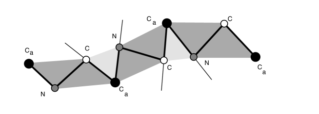
Figure 1: A panel-and-hinge model for a protein backbone sequence. $C_{\alpha}$ atoms are represented by black dots, $N$ atoms by grey and $C$ atoms by white dots. The peptide planes containing $C_{\alpha}-C-N-C_{\alpha}$ bonds (dark grey) alternate with planes containing bonds $N-C_{\alpha}-C$ (light grey). The axes of the structure, shown as extended line segments, run along the $N-C_{\alpha}$ and $C_{\alpha}-C$ bond vectors.

This situation appears for molecular conformations in $R^{3}$, when part of a molecule rotates with respect to the remaining part around an axis corresponding to a chemical bond. Figure 1 schematically represents a piece of a protein backbone [BT] as a panel-and-hinge structure.

We consider ordered chains of $n$ bodies or codimension-one panels $B_{i},\ i=1,\cdots,n$, which are articulated serially by $n-1$ hinges $A_{j},\ j=1,\cdots,n-1$, with hinge $A_{j}$ linking $B_{j}$ and $B_{j+1}$. From now on, hinge axes will be simply called hinges or axes and will refer to the corresponding codimension-two affine subspace of the chain configuration.

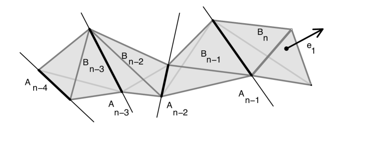
Figure 2: End part of a body-and-hinge chain in $R^{3}$, with successive bodies identified as tetrahedra $B_{j},B_{j+1}$, hinged along a common edge supported by the axis line $A_{j}$. The last body $B_{n}$ has a (rigidly) attached one-frame indicated by the vector $e_{1}$ (with given origin and direction relative to $B_{n}$).

We assume that our abstract objects (bodies or panels) can move through one another. By identifying configurations which differ only by some rigid motion of the whole chain, the total configuration space is naturally parametrized by the $(n-1)$-torus $(S^{1})^{n-1}$. We factor out these rigid motions by fixing the first object. This also fixes the first hinge. Clearly, a chain of hinged panels is simply a chain of hinged bodies subject to the condition that two consecutive hinge axes span only a codimension-one affine subspace (the corresponding panel).

To the last object, we may attach some frame (e.g. a point, or a Cartesian $k$-frame) or some flag (i.e. a sequence of linear subspaces, one included in the next), and study the end-frame or end-flag map which takes a configuration to its corresponding frame or flag position. Note that the target is itself a manifold (of frames or flags) and the resulting map is differentiable.

We study the singularities, or critical points of such maps, that is configurations corresponding to a drop in the rank of the differential. We obtain geometrical characterizations of these singularities (Theorems 1, 3, 3, 4) valid in arbitrary dimension $d$: they relate singular configurations to a lower dimensional span of the hinges in the corresponding projective Grassmann variety $G(d-1,d+1)\subset P_{{d+1\choose 2}-1}$. The most intuitive case, which was known in Robotics [SDH, Bur1, Bur2], is the end-point map in dimension 3, illustrated below.

Consider a body-and-hinge chain in $R^{3}$, with the first body fixed (i.e. identified with the ambient $R^{3}$) and with a marked point $e$ on the last body $B_{n},\ n>3$. Consider the end-point map:

$$e:(S^{1})^{n-1}\rightarrow R^{3}\ ,\ \ \theta=(\theta_{1},...,\theta_{n-1})\mapsto e(\theta)$$

which registers, for a given configuration $\theta$ of the chain, the corresponding position $e(\theta)$ of the marked point in the ambient space $R^{3}$.

Then, the the differential of this map:  $de(\theta)$ is of rank $<3$ if and only if there’s a line through the end-point $e(\theta)$ which is projectively incident with all the axes $A_{i}(\theta),\ i=1,...,n-1$ of the corresponding configuration.

Projectively incident means intersecting in $R^{3}$ or parallel, that is: intersecting ‘at infinity’ in the projective completion $P_{3}=R^{3}\sqcup P_{2}$.

It should be emphasized that the intervention of a projective characterization of singularities is no accident - indeed, it echoes the known “projective invariance of infinitesimal rigidity” in kinematics. See e.g. [Wun] [Weg].

We remark that, in dimension two, a body-and-hinge chain is as much as a panel-and-hinge chain, namely: a linkage given by $n$ rigid bars connected serially by revolute joints. This is, in other words, a planar robot arm and the singularities of the end-point map are known to be precisely the configurations with all bars along the same line [Ha] [KM1], which indeed is the content of our result in dimension two. Thus, our hinge structures may be envisaged as higher dimensional versions of simple planar linkages. Although there is a conversion dictionary between a hinge-structure description and a linkage description in arbitrary dimension - as we outline in Section 5, the former language seems better suited for characterizing singularities. We reinforce this aspect by discussing in Section 7 a related case in kinematics: infinitesimally flexible platforms.

The results in this paper have been presented at the Eighth International Symposium on Effective Methods in Algebraic Geometry (MEGA) 2005, Porto Conte, Alghero, Sardinia, May 26-June 2, 2005.

1 The end-point map for body-and-hinge chains in $R^{d}$

Let $B_{1},...,B_{n}$ denote $d$-dimensional bodies in $R^{d}$. To be precise, one should think of each $B_{i}$ as a copy of $R^{d}$, free to move relative to the ambient $R^{d}$. One may attach a Cartesian frame to the copy and represent the movement of the body as the movement of the frame.

We put a hinge $A_{j}$ between $B_{j}$ and $B_{j+1},\ j=1,...,n-1$, that is: we distinguish a codimension-two affine subspace ( an axis) in $B_{j}$ and one in $B_{j+1}$, and we specify an isometry between them, and the two linked bodies are now supposed to be positioned in the ambient $R^{d}$ subject to the condition that the two marked axes coincide, and realize the specified isometry. The common axis, as seen in the ambient $R^{d}$, or on each of the bodies so linked, will be denoted $A_{j}$.

We shall identify the first body with the ambient $R^{d}$, i.e. fix it as the reference body, because we are interested in configurations only up to a rigid motion of the assembled chain.

Clearly a hinge between two bodies allows one to rotate with respect to the other, with the hinge axis remaining pointwise fixed. This relative motion is parametrized by the unit circle $S^{1}$. Thus, with $B_{1}$ fixed, the configuration space of the chain of $n$ hinged bodies is parametrized by $(S^{1})^{n-1}$.

We distinguish now some particular point of the last body in the chain:  $e\in B_{n}-A_{n-1}$, and call it the end-point. (Obviously, we may assume $e$ to be away from the last axis $A_{n-1}$, since otherwise we would restrict considerations to $n-1$ bodies.) This produces a map (to be denoted by $e$ as well):

$$e:(S^{1})^{n-1}\rightarrow R^{d}\ ,\ \ \theta=(\theta_{1},...,\theta_{n-1})\mapsto e(\theta)$$

which associates to a configuration $\theta$, the position $e(\theta)$ of the end-point with respect to the ambient space i.e. $B_{1}$. This will be our end-point map.

Our first concern is to describe the singularities of the end-point map, that is: the configurations $\theta\in(S^{1})^{n-1}$ where the tangent map $de(\theta)$ has rank strictly less than its generic rank. We have:

$rk(de(\theta))<d$ if and only if there’s a line through $e(\theta)$ which is projectively incident with all the axes $A_{i}(\theta),i=1,...,n-1$ of the corresponding configuration.

Note that $A_{1}(\theta)=A_{1}$ is fixed, and the line through the end-point in the theorem is either intersecting an axis or parallel to it (i.e. meeting it “at infinity”, when we complete $R^{d}$ to the projective space $P_{d}$).

Proof: The image of the differential $de(\theta)$ is spanned by the tangent vectors at $e(\theta)$ to the circles (or circles degenerated to a point) described by the end-point $e(\theta)$ in the ambient $R^{d}$, when rotated around each axis $A_{i}(\theta)$.

This span is less than the full tangent space $R^{d}$ at $e(\theta)$ if and only if there’s a line $\nu$ through $e(\theta)$, normal to it. But $\nu$, will then be projectively incident with all axes.

Indeed, if $e(\theta)$ happens to be on some axis, there’s nothing to prove for that axis, while otherwise, $\nu$ must lie in the hyperplane spanned by the axis under consideration, say $A_{k}(\theta)$ and $e(\theta)$, which is the hyperplane normal to to the tangent at $e(\theta)$ for the circle described while rotating around $A_{k}(\theta)$. This is, essentially, a partial derivative at $\theta$.

By the same elementary theorem, if a line $\nu$ passing through $e(\theta)$ is projectively incident with all axes, it will be normal to $im(de(\theta))$.    $\Box$

The space orthogonal to $im(de(\theta))$ is swept by all lines through the end-point $e(\theta)$ which are projectively incident to all axes $A_{i}(\theta),\ i=1,...,n-1$.

For $n>d$ and a generic choice of hinge axes, the differential of the end-point map is generically onto, and its singularities are precisely the configurations which allow some line through the end-point to be projectively incident with all axes.

Remarks: i) The geometric argument used above does not even require to be specific about the parametrization of the configuration space by $(S^{1})^{n-1}$, e.g. what position is considered for $\theta=(0,..,0)$. It is enough to follow the infinitesimal displacements of the end-point resulting from rotating as one body the part of the chain from $B_{i}$ on, around $A_{i-1}$.

ii) This approach also shows that for infinitesimal considerations, the order of the axes may turn out to be irrelevant, while clearly essential otherwise.

iii) We have emphasized in our statements the purely projective characterization of the singularities. This is consistent with, in fact tantamount to the related phenomenon for linkages (cf. the so-called “projective invariance of infinitesimal rigidity” [Weg]).

For chains of hinged panels in $R^{3}$, the line $\nu$ in the theorem must either pass through the projective intersection of the two axes of an intermediate panel, or be contained in it; and is always contained in the last panel.

2 $k$-frames in $R^{d}$ and end-frame maps

We begin by reviewing a few facts about the homogeneous manifolds $W(k,d)$ defined by all orthogonal (i.e. Cartesian) $k$-frames in $R^{d}$.

One such frame consists of a point in $R^{d}$ (to be thought of as the origin of the frame) and $k$ ordered unit vectors which are mutually orthogonal.

Clearly, for $k=d$, we can identify the manifold $W(d,d)$ of all $d$-frames in $R^{d}$ with the isometry group $Isom(R^{d})$ of $R^{d}$:

$$W(d,d)=R^{d}\rtimes O_{R}(d)\approx Isom(R^{d})$$

where $O_{R}(d)$ stands for the real orthogonal group in dimension $d$, consisting of all orthogonal $d\times d$ matrices. (The columns of an orthogonal matrix are the vectors of a $d$-frame.) The pair $(t,M)$ gives the isometry:  $x\mapsto Mx+t$.

Suppose now $0\leq k\leq d$, and note that one can parametrize all systems of $k$ ordered, mutually orthogonal unit vectors in $R^{d}$ by the homogeneous space $O_{R}(d)/O_{R}(d-k)$ (where $O_{R}(d-k)$ is identified with the subgroup of $O_{R}(d)$ fixing the first $k$ vectors in the standard basis). (These homogeneous spaces are called Stiefel manifolds.) This gives the general description:

$$W(k,d)=R^{d}\rtimes O_{R}(d)/O_{R}(d-k)\approx Isom(R^{d})/O_{R}(d-k)$$

$$dim_{R}W(k,d)=d+{d\choose 2}-{{d-k}\choose 2}={{d+1}\choose 2}-{{d-k}\choose 2}$$

Notice that there’s a natural action of the group of isometries in dimension $k$:  $Isom(R^{k})$, on the space of $k$-frames in $R^{d}$:  $W(k,d)$.

$$Isom(R^{k})\times W(k,d)\rightarrow W(k,d)$$

A $k$-frame gives an identification of its span with $R^{k}$, and $Isom(R^{k})$ acts by displacing the given frame to the image of the standard basis. Thus the action preserves the $k$-plane spanned by a frame (through its origin), that is: a $k$-frame and its transforms have the same ‘supporting’ $k$-plane.

Let us fix a $k$-frame $E_{k}$ in the last body $B_{n}$ of a hinged chain. As in the case of a point $e=E_{0}$, this gives an end-frame map:

$$(S^{1})^{n-1}\rightarrow W(k,d),\ \ \theta\mapsto E_{k}(\theta)$$

takig a configuration $\theta$ to the corresponding position of the end $k$-frame in the ambient $R^{d}$.

Again, for the singularities of the end-frame map, only the positions of the axes matter, not their ordering, and the remarks on the action of $Isom(R^{k})$ on $W(k,d)$ give:

The singularities of the end-frame map:

$$E_{k}:(S^{1})^{n-1}\rightarrow W(k,d),\ \ \theta\mapsto E_{k}(\theta)$$

depend only on the set of axes and the $k$-plane spanned by the end-frame.

It may be useful in this context to cosider explicitly the map which takes a $k$-frame to the (affine) $k$-plane it spans in $R^{d}$, as a map to the Grassmann variety $G(k+1,d+1)$ parametrizing all $(k+1)$ linear subspaces in $R^{d+1}$, that is: all projective $k$-planes in $P_{d}$:

$$\pi_{k}:W(k,d)\rightarrow G(k+1,d+1)$$

The axes themselves can be seen as points in $G(d-1,d+1)\approx G(2,d+1)$, and our proposition says that the singularities of the end-frame map depend only on $A_{i}(\theta),i=1,...,n-1$, and $\pi_{k}(E_{k}(\theta))$ as a point of $(G(d-1,d+1)^{n-1}/{\cal S}_{n-1})\times G(k+1,d+1)$.

In order to see what kind of geometrical characterization of singularities should emerge, we look in the next section at the case $k=d-2$. A $(d-2)$-frame on the last body may be interpreted as a ‘loose hinge’, or half a hinge, and if we prescribe its matching half i.e. a $(d-2)$-frame in the ambient $R^{d}$ (which is the first body), we may interpret the fibers of the end-frame map $E_{d-2}$, as configuration spaces of cycles of $n$ hinged bodies, for various placements of the closing hinge.

3 From chains to cycles

When we take $k=d-2$, Proposition 2.1 says that the singularities of $E_{d-2}$ depend on corresponding configurations of $n$ points in the Grassmann variety $G(d-1,d+1)$. Since the singularities of the map indicate singularities of the fibers, and the fibers, in this case, are cycles of $n$ bodies with $n$ hinges, we see that the order of the $n$ points in the Grassmannian is not actually relevant.

We should add the remark that our set-up generalizes the case $d=2$ of the planar ‘robot arm’ and planar polygon spaces [Ha] [KM1] [Bor2]. In that case, one has singularities if and only if all $n$ axes (which are simply points in $R^{2}\subset P_{2}$) are collinear. In general, we have:

Suppose $n\geq{{d+1}\choose 2}$. Consider the Plücker embedding of the Grassmann variety:

$$G(d-1,d+1)\hookrightarrow P_{{{d+1}\choose 2}-1}$$

The end-frame map for a chain of $n$ hinged bodies in $R^{d}$:

$$E_{d-2}:(S^{1})^{n-1}\rightarrow W(d-2,d)$$

has a singularity at $\theta\in(S^{1})^{n-1}$ if and only if the $n$ points of $G(d-1,d+1)$ corresponding to the axes $A_{i}(\theta)$, $i=1,...,n-1$ and the span $\pi_{d-2}E_{d-2}(\theta)$ of the end-frame, all lie in some hyperplane section of the Grassmannian (in its Plücker embedding).

Note that:  $dim_{R}W(d-2,d)={{d+1}\choose 2}-1$.

In terms of cycles, we have the simpler, but equivalent formulation:

The configuration space parametrizing the possible positions (up to Euclidean motions) of a cycle of $n\geq{{d+1}\choose 2}$ hinged bodies in $R^{d}$ is singular whenever the $n$ axes, as points in

$$G(d-1,d+1)\hookrightarrow P_{{{d+1}\choose 2}-1}$$

span less than the whole ambient projective space of the Grassmannian.

Note that a generic (initial) position of the $n$ axes gives a configuration space of dimension $n-{{d+1}\choose 2}$.

Proof: We extend the argument presented by Bricard in Tome II, Note H of [Br2].

An infinitesimal motion of our chain of $n$ hinged bodies in $R^{d}$ corresponds with relative infinitesimal motions for each couple:

$$(B_{2}/B_{1})\ (B_{3}/B_{2})\ ...(B_{n}/B_{n-1})(B_{1}/B_{n})$$

which are all tangent to uniform rotations with axes $A_{1},...,A_{n}$.

A simple way to encode a uniform rotation around a codimension two axis $A_{i}\subset R^{d}$ uses an arbitrary point $M_{i}\in A_{i}$ and an element $\omega_{i}=v^{i}_{1}\wedge v^{i}_{2}\wedge...\wedge v^{i}_{d-2}\in\bigwedge^{d-2}R^{d}$, where $v^{i}_{1},...,v^{i}_{d-2}$ is a basis of the subspace $A_{i}-M_{i}$, whose exterior power $\omega_{i}$ represents the angular velocity of the rotation.

The information $(M_{i},\omega_{i})$, which generalizes the notion of sliding vector (vecteur glissant) in dimension three, can also be presented as an exterior vector:

$$T_{i}=0_{d}M_{i}\wedge\omega_{i}+e_{d+1}\wedge\omega_{i}=0_{d+1}M_{i}\wedge\omega_{i}\in\bigwedge^{d-1}R^{d+1}$$

when we consider $R^{d}$ as the affine subspace $x_{d+1}=1$ in $R^{d+1}$ with the origin $0_{d}=(0,...,0,1)$, so that $e_{d+1}=0_{d+1}0_{d}$. Thus uniform rotations become representatives for points in $G(d-1,d+1)$ determined by their (affine) axes.

The component $0_{d}M_{i}\wedge\omega_{i}$ in $T_{i}$ expresses the velocity of $0_{d}\in R^{d}$ rotating with respect to $A_{i}$.

When we fix representatives $\alpha_{i}\in\bigwedge^{d-1}R^{d+1}$ for all axes $A_{i}\in G(d-1,d+1)$, we have:  $T_{i}=\tau_{i}\alpha_{i}$.

The result of the relative infinitesimal motions given by $(M_{i},\omega_{i}),\ i=1,...,n$ on the corresponding couples $(B_{i+1}/B_{i})$ is clearly the identity when considered relative to one and the same body, say $(B_{1}/B_{1})$. Thus, generalizing the null torsor condition in dimension three, we must have:

$$\sum_{i=1}^{n}\tau_{i}\alpha_{i}=0\ \ \ \ \ \ \ \ \ (T)$$

Indeed, the resulting velocities must be zero at the origin $0_{d}$ and elswhere:

$$\sum_{i=1}^{n}0_{d}M_{i}\wedge\omega_{i}=0$$

$$\sum_{i=1}^{n}PM_{i}\wedge\omega_{i}=0\ \ \ \ i.e.\ \ \ \ \sum_{i=1}^{n}P0_{d}\wedge\omega_{i}=0\ \mbox{for any}\ P\in R^{d}$$

The last condition gives:

$$\sum_{i=1}^{n}\omega_{i}=0$$

and $(T)$ follows.

The dimension of the space of solutions $(\tau_{i})_{i}$ of equation $(T)$ is $n-rank(\alpha_{i})_{i}$, hence: the configuration space has a singularity if and only if the axes span less than the whole ambient space of the Grassmannian.    $\Box$

Remarks: In the generically rigid case for cycles, namely $n={{d+1}\choose 2}$, a singularity in the configuration space means infinitesimal flexibility.

In space $(d=3)$, we would have a cycle of 6 hinged bodies or panels. The case of 6 panels corresponds to the cyclo-hexane molecule, and when phrased in terms of linkages to 1-skeleta of octahedra. Thus, our result recovers characterizations of infinitesimal flexibility for objects of some long-standing interest [Br1], [Ben], [Br2]. A hyperplane section of the Grassmann-Plücker quadric $G(2,4)\subset P_{5}$ is also called a linear complex. A note of Darboux to Koenigs’ ‘Leçons de cinématique’, p.431, mentions a fact known to Chasles: a twisted cubic in $P_{3}$ has all its tangents in the same linear complex i.e. a rational normal cubic has all its tangents in the same hyperplane section of the Grassmannian $G(2,4)$.

Other examples of six lines in a linear complex come from Bricard’s flexible octahedra. In particular, as observed in [Ben] (sect. 17), a six-cycle in $R^{3}$ with hinges symmetric in pairs relative to an axis, has one degree of freedom of motion. To see that the hinges are linearly dependent in $G(2,4)\subset P_{5}$, note that the symmetry in a line, as a projective transformation $T$, can be given by a diagonal matrix with two $+1$ and two $-1$ eigenvalues, hence inducing an involution with two $+1$ and four $-1$ eigenvalues on $\bigwedge^{2}R^{4}$. Thus $\ell_{i}+T\ell_{i},\ i=1,2,3$ are dependent.

4 End-frame and end-flag maps

Suppose $0\leq k<d-2$, and consider a $k$-frame attached to the last body of a chain. Clearly, any extension of this $k$-frame to a $k+r$-frame gives a factorization of the end-frame map $E_{k}$ through $E_{k+r}$:

$$(S^{1})^{n-1}\rightarrow W(k+r,d)\rightarrow W(k,d)$$

The differential of the last arrow is surjective at all points, and it follows that the singularities of $E_{k}$ are contained in the singularities of $E_{k+r}$, for any extension of the end-frame. This leads to:

Let $0\leq k\leq d-2$ and $n>dim_{R}W(k,d)={{d+1}\choose 2}-{{d-k}\choose 2}$.

The end-frame map for a chain of hinged bodies in $R^{d}$:

$$E_{k}:(S^{1})^{n-1}\rightarrow W(k,d)$$

has a differential of rank less than $dim_{R}W(k,d)$ at $\theta\in(S^{1})^{n-1}$ if and only if, the $n-1$ points of the Grassmann variety $G(d-1,d+1)$ corresponding to the axes $A_{i}(\theta)$, $i=1,...,n-1$ and the locus made of $\pi_{d-2}E_{d-2}(\theta)$ for all extensions of the $k$-frame $E_{k}(\theta)$ to a $(d-2)$-frame $E_{d-2}(\theta)$, are contained in some hyperplane section of the Grassmannian (in its Plücker embedding).

For a generic initial position $\theta=0$ of the axes and the end-frame:

$$dim_{R}E_{k}^{-1}(E_{k}(0))=n-{{d+1}\choose 2}+{{d-k}\choose 2}-1$$

This statement shows that one may replace frames with flags (which is, in fact, the natural thing to do from the complex point of view), and consider the singularities of the end-flag map:

$$F_{k}:(S^{1})^{n-1}\rightarrow W(k,d)\rightarrow Fl(k,d)$$

obtained by composition with $W(k,d)\rightarrow Fl(k,d)$, which associates to an orthogonal frame $E_{k}=\{e_{0},e_{1},...,e_{k}\}$ the projective flag in $P_{d}(R)=R^{d}\cup P_{d-1}(R)$ made of subspaces spanned by the first $m$ elements in the frame, with $0\leq m\leq k$.

Proof:  We use the shorter notation $Isom(R^{k})=E(k)$. Lie algebras will be denoted with corresponding small case letters. Using the homogeneous space description:

$$W(k,d)=E(d)/O(d-k)$$

we may identify the tangent space to $W(k,d)$ at $E_{k}(\theta)$ with $e(d)/o(d-k)$.

As in our argument for Theorem 1., the image of the tangent map at $\theta$ is spanned by the $(n-1)$ tangent vectors corresponding to rotations around each axis (with the rest of the chain imagined as rigid, from that axis on). These vectors are represented in $e(d)$ by the corresponding infinitesimal rotations.

They do not span the whole tangent space $e(d)/o(d-k)$ precisely when there’s a linear functional on $e(d)$, vanishing on $o(d-k)$ and all the $(n-1)$ infinitesimal rotations.

The theorem then is simply the reading of this statement when converted via the linear isomorphism

$$e(d)\approx o(d+1)$$

and the natural identification of skew-symmetric two-forms (in $(d+1)$ variables) with $(d-1)$ exterior vectors:  $o(d+1)\approx\wedge^{d-1}(R^{d+1})$. Indeed, an infinitesimal rotation around a codimension-two axis corresponds precisely with the exterior vector representing the axis as a point of the Grassmanniann $G(d-1,d+1)$.

5 Converting cycles into linkages

In this section we describe (canonical) procedures for associating linkages with $2n$ vertices and $(2d-1)n$ edges in $R^{d}$ to generic cycles of $n$ hinged bodies in $R^{d},\ d\geq 3$. This association will permit the identification of the cycle configuration space with corresponding components of the linkage configuration space.

The indices for axes and bodies should be understood cyclically i.e. modulo $n$.

We need to distinguish between the case of odd and even dimension.

Suppose $d$ is odd, that is: $d=2k+1$. In the generic case, all intersections of $k$ consecutive axes are lines.

$$l_{i}=A_{i}\cap A_{i+1}\cap...\cap A_{i+k-1}$$

One should regard $l_{i}$ as part of $A_{i}$ (and moving with it as the cycle deforms into other configurations).

We choose two points in general position on each of these $n$ lines. This gives exactly $2k$ points on each axis, and exactly $2k+2$ points on any pair of consecutive axes, which corresponds to a body. Thus, the $d$-simplex generated by the $2k+2$ points marks the body, and we take as edges in our linkage all edges belonging to one of these $n$ simplices. A final count gives $(2d-1)n$ edges.

Remark: There is, in fact, a canonical way to choose two points on each of the above lines. Indeed, for every pair of consecutive lines, there’s a unique common perpendicular incident to both, and this gives one point on each line in the pair. In the end, one has two points on each line.

Suppose now $d$ even, that is: $d=2k$. In the generic case, all intersections of $k$ consecutive axes are points:

$$p_{i}=A_{i}\cap A_{i+1}\cap...\cap A_{i+k-1}$$

We consider these $n$ points $p_{i}$, together with $n$ points chosen generically, one in each intersection of $k-1$ consecutive axes:

$$q_{i}\in A_{i}\cap A_{i+1}\cap...\cap A_{i+k-2}$$

This gives exactly $2k-1$ points in each axis, and $2k+1$ points in any pair of two consecutive axes. As in the odd case, this leads to a linkage with $2n$ vertices and $(2d-1)n$ edges which is the 1-skeleton of a complex consisting of $n$ simplices of dimension $d$ which share cyclically, one with the next, a $(d-2)$-face.

Remark: Again, the generic case allows for a canonical choice of the points $q_{i}$. Indeed, one may define $q_{i}$ as the orthogonal projection of $p_{i+1}$ on the plane $A_{i}\cap A_{i+1}\cap...\cap A_{i+k-2}$.

For more definiteness, we recall the notions of configuration space envisaged here for cycles of hinged bodies, respectively linkages.

For cycles, we consider an initial position of axes $A_{i}=A_{i}(0)\subset R^{d},\ i=1,...,n$. Every pair of consecutive axes $(A_{i},A_{i+1})$ belongs to a rigid body $B_{i+1}$, understood as a copy of $R^{d}$. $B_{i+1}$ can move relative to $B_{i}$ by rotating with respect to the common axis $A_{i}$. We consider $B_{1}$ identified with the ambient $R^{d}$, fix a $(d-2)$-frame in $A_{n}$, and define the configuration space ${\cal C}(A_{1},...,A_{n})$ for our initial position $\theta=0$ as the fiber of the end-frame map $E_{d-2}$ over the initial position $E_{d-2}(0)$. (See sections 2 and 3 above.) In formulae:

$$E_{d-2}:(S^{1})^{n-1}\rightarrow W(d-2,d)$$

with $E_{d-2}(0)$  a  $(d-2)$-frame in $A_{n}=A_{n}(0)$, and:

$${\cal C}(A_{1},...,A_{n})=E_{d-2}^{-1}(E_{d-2}(0))$$

The configuration space so defined is (up to canonical identifications) independent of the end-frame chosen in $A_{n}$, or a cyclic permutation of the indices.

Our results in section 3 imply that, for a generic initial position, the configuration space will be a smooth submanifold of $(S^{1})^{n-1}$, of dimension $n-{{d+1}\choose 2}$. However, this submanifold might have several connected components.

We turn now to linkages. A linkage $L$ is a weighted graph, with weights indicating the length ascribed to each edge. A realization of $L$ in $R^{d}$ is a map from the vertex set of $L$ to $R^{d}$, such that any two vertices defining an edge are placed at the distance required by its weight. The configuration space ${\cal C}(L)={\cal C}(L,d)$ of $L$ in $R^{d}$ is the space of all realizations of $L$ in $R^{d}$, modulo Euclidean motions (i.e. orintation preserving isometries of $R^{d}$). Cf.[Bor1] [B-S].

In order to emphasize the fact that our canonical procedure for converting (generic) cycles into linkages is independent of the representative chosen in describing the configuration space ${\cal C}(A_{1},...,A_{n})$, one can use the following:

Let $A=(A_{i})_{i},A^{\prime}=(A^{\prime}_{i})_{i}$ denote two configurations in ${\cal C}(A)={\cal C}(A_{1},...,A_{n})={\cal C}(A^{\prime})$, with canonically associated linkages $L(A)$ and $L(A^{\prime})$. Then:

$$L(A)=L(A^{\prime})$$

This means that their graphs can be identified, and the length ascribed to corresponding edges is the same.

Proof: The graphs, in our case, are clearly the same: 1-skeleta of identically labeled simplicial complexes. Thus, one has to verify only the edge-length matching.

To see this, we consider the simplices in the canonical realization of $L(A)$ as markers for the $n$ bodies $B_{i}$. Imagining the cycle A unhinged at $A_{n}$ (but with the $(d-2)$ simplicial face marked on both $B_{1}$ and $B_{n}$ - the equivalent of a $(d-2)$-frame), there is a continuous deformation of the chain (by some trajectory in $(S^{1})^{n-1}$ linking A to A’) which ends-up as A’ by matching again the two marked $(d-2)$ simplicial faces in $B_{1}$ and $B_{n}$. But this restores perforce all the incidences (and orthogonalities) defining the canonical realization of $L(A^{\prime})$ as incidences (and orthogonalities) of the moved simplices of $L(A)$.    $\Box$

Note:  The argument shows a little more: the corresponding simplices are not only congruent, but realized with the same orientation. In fact, the linkage configuration space ${\cal C}(L(A))$ does contain realizations with one or the other orientation for some of the simplices in the underlying complex, and our inclusion ${\cal C}(A)\subset{\cal C}(L(A))$ covers only those components where all orientations are as given in the canonical realization associated to A. Denoting this image by ${\cal C}(L(A)_{c})$, we obtain a diagram:

$\begin{array}[]{cclcc}{\cal C}(A)&\subset&(S^{1})^{n-1}&\subset&G(d-1,d+1)^{n-2}\\ \downarrow&&&&\uparrow\\ {\cal C}(L(A)_{c})&&\subset&&(P_{d})^{2n-(d+1)}\end{array}$

where, considering the first body $B_{1}$ as fixed, and the corresponding simplex with $(d+1)$ vertices in $L(A)$ fixed as well, the last column records the axes $A_{2}(\theta),...,A_{n-1}(\theta)$, respectively the remaining $2n-(d+1)$ vertices placed in $R^{d}\subset P_{d}$, and their relation through a (generically defined) rational map.

Let $A$ be a generic $n$-cycle in $R^{d}$ with axes $A_{1},...,A_{n}$. For $A_{n+1}\neq A_{n}$ sufficiently close to $A_{n}$, we have:

$${\cal C}(A_{1},...,A_{n+1})=S^{1}\times{\cal C}(A_{1},...,A_{n})$$

This is the analogon of “a small cut at a vertex” for polygon spaces. The proof, as in that case, amounts to observing that the fibers of the end-frame map:

$$E_{d-2}:(S^{1})^{n-1}\rightarrow W(d-2,d)$$

over a small neighborhood of $E_{d-2}(0)$ can be identified with ${\cal C}(A_{1},...,A_{n})=E_{d-2}^{-1}(E_{d-2}(0)$.    $\Box$

6 Cycle invariants: moduli

When we look at $n$-cycles as points in $G(d-1,d+1)^{n}$ modulo the diagonal action of the group of Euclidean motions in $R^{d}$, we have a parameter space of dimension $2(d-1)n-{{d+1}\choose 2}$ containing cycle configuration spaces of generic dimension $n-{{d+1}\choose 2}$. Thus, a parameter space for the cycle configuration spaces, that is: a moduli space, should have dimension $(2d-3)n$. In other words, we expect $(2d-3)n$ continuous parameters (also called invariants or moduli), to characterize a generic configuration space, at least up to a finite number of possibilities.

Example:  For the planar case $(d=2)$, with $n$-cycles understood as $n$-gons with prescribed edges, the obvious invariants are the edge lengths themselves. The admissible edge-length-vectors make-up a polyhedreal cone in $R^{n}$ (with section a second hypersimplex). The various topological types for planar polygon configuration spaces are then described in terms of a subdivision into chambers of this cone. [Bor2] [Ha] [KM1] [N]

According to the previous section, the canonical linkage $L(A)$ associated to a generic cycle $A=(A_{1},...,A_{n})\in{\cal C}(A)$ may be envisaged as an invariant of the cycle configuration space in dimension $d\geq 3$. This gives, upfront, $(2d-1)n$ edge lengths, but we have a number of orthogonalities in all canonical realizations, which make $2n$ distances dependent on the remaining $(2d-3)n$. Thus, one obtains $(2d-3)n$ invariants. However, the cone they determine in $R^{(2d-3)n}$ is more complicated than in the planar case.

Obviously rescaling does not change the structure of the configuration spaces, and we may replace the cone with a transversal section of dimension $(2d-3)n-1$, corresponding to ratios of invariants.

7 Platforms

In this section we present a complementary result in kinematics, meant to emphasize the fact that line geometry (or dually, axis geometry), that is: the use of Grassmann varieties $G(2,d+1)\approx G(d-1,d+1)$, provides a natural context for singularity issues.

Our example may be envisaged as a generalization of a theorem of Desargues, form the ‘perspective’ of ‘platforms’. For background on infinitesimal rigidity we refer to [B-S] and [Weg].

A platform in $R^{d}$ consists of two (rigid) bodies connected by ${{d+1}\choose 2}$ rigid bars with ends $p_{ij}$ on one body, respectively $q_{ij}$ on the other. For $d=2$ we connect the vertices of two triangles with three bars, and the resulting framework is infinitesimally flexible precisely when the triangles are in perspective for the given pairing of vertices: in other words, they produce a Desargues configuration. This generalizes to:

A platform in dimension $d$ is infinitesimally flexible if and only if the ${{d+1}\choose 2}$ lines defined by the connecting bars $p_{ij}q_{ij}$ lie in a hyperplane section of the Grassmannian $G(2,d+1)\subset P_{{{d+1}\choose 2}-1}$.

Proof; We use a ‘projective’ version of the paltform, by imagining $R^{d}$ as $x_{0}=1$ in $R^{d+1}$ and the origin linked by bars to $p_{ij}$ and $q_{ij}$. We may consider the first body fixed, and the infinitesimal motion of the second given by an anti-symmetric $(d+1)\times(d+1)$ matrix $A$. An infinitesimal motion of the platform requires:

$$<Aq_{ij},p_{ij}-q_{ij}>=0\ \ i.e.\ \ <Aq_{ij},p_{ij}>=0$$

and this linear system in the unknowns $a_{ij}$ has a non-trivial solution precisely when the exterior two-vectors:  $p_{ij}\wedge q_{ij}$, $1\leq i<j\leq(d+1)$ are linearly dependent.    $\Box$

Remark: For the ‘Stewart-Gough platform’ i.e. $d=3$, this fact is presented in [RV], following [Mer].

8 Conclusions

In principle, understanding the singularities of a map offers a key towards the topology of its fibers (usually via some Morse theory), and this approach is common to a number of studies on mechanical linkages [N] [Ha] [KM1] [KM2] [Bor2].

One should also remark that, with configuration spaces of this nature, all relevant maps are algebraic, and this allows the intervention of complex algebraic-geometry, as in [Kly] [Bor2].

References

- [Ben] Bennett, G.T.: Deformable octahedra, Proc. London Math. Soc. 10 (1911), 309-343.
- [Bor1] Borcea, C.S.: Point configurations and Cayley-Menger varieties, preprint arXiv: math.AG/0207110.
- [Bor2] Borcea, C.S.: Polygons spaces, tangents to quadics and special Lagrangians, in Oberwolfach Reports, Komplexe Analysis, vol. 1, no. 3 (2004).
- [B-S] Borcea, C.S. and Streinu, I.: The number of embeddings of minimally rigid graphs, Discrete and Computational Geometry 31 (2004), 287-303.
- [BT] Braden, C. and Tooze, J.: Introduction to Protein Structure, 2nd edition, Garland Publishing, Inc., New York (1998).
- [Br1] Bricard, R.: Mémoire sur la théorie de l’octaèdre articulé, J. Math. Pure et Appl. 5 (1897), 113-148.
- [Br2] Bricard, R.: Leçons de cinématique, Tome I (1926), Tome II (1927), Gauthier-Villars, Paris.
- [Bur1] Burdick, J.W.: A classification of 3R regional manipulator singularities and geometries, Mechanism and Machine Theory 30, no.1 (1995), 71-89.
- [Bur2] Burdick, J.W.: A recursive method for finding revolute-jointed manipulator singularities, Transactions of the ASME, Journal of Mechanical Design 117 (1995), 55-63.
- [CP] Canny, J. and Parsons, D.: Geometric problems in molecular biology and robotics, Proceedings of the Second International Conference on Intelligent Systems for Molecular Biology, Stanford, CA, 1994.
- [G] Guest, M.: Morse theory in the 1990’s, in Invitations to geometry and topology, Oxford Grad. Texts Math. 7, Oxford Univ. Press (2002), 146-207.
- [Ha] Hausmann, J-C.: Sur la topologie des bras articulés. In “Algebraic Topology, Poznan”, Springer Lectures Notes 1474 (1989), 146-159.
- [HK1] Hausmann, J-C. and Knutson, A.: Polygon spaces and Grassmannians. L’Enseignement Mathématique 43 (1997), 173-198
- [HK2] Hausmann, J-C. and Knutson, A.: The cohomology ring of polygon spaces Ann. Inst. Fourier 48 (1998), 281-321.
- [KM1] Kapovich, M. and Millson, J.: On the moduli space of polygons in the Euclidean plane. J. Diff. Geom. 42 (1995), 431-464.
- [KM2] Kapovich, M. and Millson, J.: The symplectic geometry of polygons in Euclidean space. J. Diff. Geometry 44 (1996), 479-513.
- [Kly] Klyachko, A.: Spatial polygons and stable configurations of points in the projective line. In: Algebraic geometry and its applications (Yaroslavl, 1992), Aspects of Math., Vieweg, Braunschweig (1994), 67-84.
- [Koe] Koenigs, G.: Leçons de cinématique, (1897) Hermann, Paris.
- [Mer] Merlet, J.-P.: Singular configurations of parallel manipulators and Grassmann geometry, in “Geometry and Robotics” (ed. by J.-D. Boissonnant and J.-P. Laumond), Lecture Notes in Computer Science, vol. 391, Springer Verlag (1989).
- [M] Milnor, J.: Morse Theory, Annals of Mathematics Studies, vol. 51, Princeton University Press, 1963.
- [N] Niemann, S.H.: Geometry and mechanics. Thesis. St. Catherine’s College, Oxford (1978).
- [RV] Ronga, F. and Vust, T.: Stewart platform without computer?, in “Real Analytic and Algebraic Geometry”, Proc. Int. Conf. (Trento,1992), Walter de Gruyter (1995), 196-212.
- [Se] Selig, J.M.: Geometric Methods in Robotics, Springer-Verlag, New York (1996).
- [SDH] Sugimoto, K., Duffy, J. and Hunt, K.H.: Special configurations of spatial mechanisms and robot arms,Mechanism and Machine Theory 17, no.2 (1982), 119-132.
- [Weg] Wegner, B.: On the projective invariance of shaky structures in Euclidean space, Acta Mechanica 53 (1984), 163-171.
- [Wun] Wunderlich, W.: Projective invariance of shaky structures, Acta Mechanica 42 (1982), 171-181.