Microstate Dependence of

Scattering from the D1-D5 System

Sumit R. Das

Department of Physics and Astronomy,

University of Kentucky, Lexington, KY 40506 USA

Gautam Mandal

Department of Theoretical Physics,

Tata Institute of Fundamental Research,

Mumbai 400 005, INDIA

das@pa.uky.edu, mandal@theory.tifr.res.in

Abstract

We investigate the question of distinguishing between different microstates of the D1-D5 system with charges $Q_{1}$ and $Q_{5}$, by scattering with a supergravity mode which is a minimally coupled scalar in the leading supergravity approximation. The scattering is studied in the dual CFT description in the orbifold limit for finite $R$, where $R$ is the radius of the circle on which the D1 branes are wrapped. Even though the system has discrete energy levels for finite $R$, an absorption probability proportional to time is found when the ingoing beam has a finite width $\Delta E$ which is much larger than the inverse of the time scale $T$. When $R\Delta E\gg 1$, the absorption crosssection is found to be independent of the microstate and identical to the leading semiclassical answer computed from the naive geometry. For smaller $\Delta E$, the answer depends on the particular microstate, which we examine for typical as well as for atypical microstates and derive an upper bound for the leading correction for either a Lorentzian or a Gaussian energy profile of the incoming beam. When $1/R\gg\Delta E\gg$ the average energy gap $\left(1/(R\sqrt{Q_{1}Q_{5}})\right)$, we find that in a typical state the bound is proportional to the area of the stretched horizon, ${\sqrt{Q_{1}Q_{5}}}$, up to $\log(Q_{1}Q_{5})$ terms. Furthermore, when the central energy in the incoming beam, $E_{0}$, is much smaller than $\Delta E$, the proportionality constant is a pure number independent of all energy scales. Numerical calculations using Lorentzian profiles show that the actual value of the correction is in fact proportional to ${\sqrt{Q_{1}Q_{5}}}$ without the logarithmic factor. We offer some speculations about how this result can be consistent with a resolution of the naive geometry by higher derivative corrections to supergravity.

1 Introduction and Summary

The two charge system, particularly in the duality frame in which it is a bound state of $Q_{1}$ D1 branes and $Q_{5}$ D5 branes, has served as a useful theoretical laboratory for understanding the physics of black holes in string theory. In fact, this system (in the duality frame in which this is a fundamental heterotic string with some momentum), provided the first evidence that string theory states can account for black hole entropy [2].

When the D5 branes are wrapped on a $T^{5}$ and the D1 branes are wrapped on an $S^{1}$ (of radius $R$) contained in the $T^{5}$, the microscopic description of the system at low energies is that of a $(4,4)$ superconformal field theory with a target space which is a resolution of the orbifold $(T^{4})^{N}/S(N),\ N=Q_{1}Q_{5}$[3, 4, 5, 6, 7]. In the orbifold limit, the SCFT consists of $N=Q_{1}Q_{5}$ copies of free bosonic fields $X^{a}$ and their fermionic partners $\psi^{\alpha}$, $a=1,..,4;\alpha=1,...,4$, in various twist sectors corresponding to elements of $S(N)$. Any given element of $S(N)$ can be described by multiple copies of the cyclic permutation $Z_{n}$ , for various values of $n=1,...N$ (up to equivalence). A given twist sector, therefore, corresponds to specific multiplicities $N_{n,\mu}$ ($N^{\prime}_{n,\mu}$) of the $Z_{n}$ twists acting on the bosons (fermions), where $\mu=1\cdots 4$ denotes a polarization index. The numbers $\{N_{n,\mu},N^{\prime}_{n,\mu}\}$ are constrained to satisfy

$$\sum_{n=1}^{N}n\,N_{n}=Q_{1}Q_{5}\equiv N,\quad N_{n}\equiv\sum_{\mu}N_{n,\mu}+\sum_{\mu}N^{\prime}_{n,\mu}$$ (1)

For periodic boundary condition around the circle, the SCFT is described by the Ramond sector. The 2-charge system consists of the various degenerate Ramond ground states, one from each twist sector. Thus the entropy of the 2-charge system is given by

$$S=\log\Omega$$ (2)

where $\Omega$ is total number of twist sectors, or in other words the number of possible sets of values of $\{N_{n,a},N_{n,\alpha}\}$ subject to the condition (1). For large $N$, this is given by

$$S=2\pi\sqrt{2N}$$ (3)

In two derivative supergravity, the standard description of this system is in terms of a string frame metric

$$ds^{2}=(f_{1}(r)f_{5}(r))^{-1/2}[-dt^{2}+dy^{2}]+(\frac{f_{1}(r)}{f_{5}(r)})^{1/2}[dx_{1}^{2}+\cdots dx_{4}^{2}]+(f_{1}(r)f_{5}(r))^{1/2}[dr^{2}+r^{2}d\Omega_{3}^{2}]$$ (4)

where the harmonic functions are given by

$$f_{1}(r)=1+\frac{r_{1}^{2}}{r^{2}}=1+\frac{16\pi^{4}g_{s}l_{s}^{6}RQ_{1}}{Vr^{2}}~{}~{}~{}~{}~{}~{}~{}~{}f_{5}(r)=1+\frac{r_{5}^{2}}{r^{2}}=1+\frac{g_{s}l_{s}^{2}\,Q_{5}}{r^{2}}$$ (5)

We will call this the “naive” geometry. The dilaton and the gauge fields are

$$e^{-2\Phi}=\frac{f_{5}(r)}{f_{1}(r)}~{}~{}~{}~{}~{}~{}A_{01234y}=\frac{1}{2}(1-f_{5}^{-1})~{}~{}~{}~{}~{}~{}A_{0y}=\frac{1}{2}(1-f_{1}^{-1})$$ (6)

Here $l_{s}$ is the string length, $g_{s}$ is the string coupling, $R$ is the radius of the $y$ direction and $V$ denotes the coordinate volume of the $T^{4}$ along the directions $x^{1}\cdots x^{4}$. The area of the horizon, at $r=0$, vanishes because the size of the $y$ direction vanishes here - so that there is no Bekenstein-Hawking entropy. However, as was shown in [2], the area of the stretched horizon, argued to appear from $\alpha^{\prime}$ corrections, reproduces the microscopic entropy up to a numerical factor.

More recently it has been realized that once higher derivative terms in supergravity are included, the naive geometry of similar 2-charge systems gets significantly modified: a finite horizon develops and the Wald entropy of this latter geometry precisely agrees with the microscopic answer [8, 9]. While this has not been shown for the D1-D5 system on $T^{4}$ which we are considering, it is reasonable to expect that a finite horizon should again develop and the Wald entropy would again agree, at least up to proportionality, with the microscopic entropy.

The near-horizon geometry of (4) is locally $AdS_{3}\times S^{3}\times T^{4}$ with an identification $y\sim y+2\pi R$. The AdS scale $\ell$ is given by

$$\ell^{4}=(r_{1}r_{5})^{2}=\frac{16\pi^{4}g_{s}^{2}l_{s}^{8}N}{V}=\frac{\kappa^{2}N}{4\pi^{3}V}$$ (7)

where $\kappa$ denotes the ten dimensional gravitational coupling constant, related to ten dimensional Newton’s constant $G_{10}$ by $\kappa^{2}=8\pi G_{10}$. By virtue of the standard AdS/CFT correspondence, string theory on this geometry is dual to the (4,4) SCFT on the resolved orbifold.

In a different direction, Mathur and collaborators have found smooth horizon-free solutions of leading order supergravity corresponding to CFT states of the system [10, 11]. These “fuzzball” solutions become identical to the naive geometry at large $r$, but start deviating from it at values of $r\sim(Q_{1}Q_{5})^{1/6}-$ which is where a stretched horizon should be located. The fuzzball program has been extended to other systems for which the leading order supergravity solution has a finite horizon area, e.g. the 3 charge system in five dimensions [12].

Geometries with horizons, e.g. the naive geometry (4) with a singular horizon, or those with a regular horizon [8, 9] obtained in higher derivative supergravity, should be in some sense [11] coarse-grained descriptions of the fuzzball geometries. It is clearly important to understand the precise meaning of this averaging process. This issue has been studied from various viewpoints, both in the present context of the D1-D5 system [18, 19, 20] as well as in a similar context of BPS states in $AdS_{5}$ [13, 14, 15, 16, 17]. In particular, [18] and [19] studied correlation functions in the orbifold limit of CFT and showed that for typical microstates and short time scales these are independent of the details of the microstate and that they agree, under AdS/CFT, with the naive supergravity (BTZ) answers at short time scales. The agreement does not work for atypical microstates or long time scales.

In this paper we investigate this problem from a different point of view. We consider in detail the scattering of certain low energy supergravity probes off the D1-D5 system at a finite radius $R$ and ask how, if at all, we can figure out the microstate-dependence from the $R$-dependent absorption crosssection. The expectation stems from the fact that at finite $R$ the CFT spectrum is discrete and the nature of the discreteness carries information about the specific microstate the system is in.

In carrying out this study, we encounter a subtlety, viz. that a system with discrete energy levels never absorbs a monochromatic incident wave at a constant rate, i.e. the probability of transition to an excited state never becomes proportional to time. One way to obtain a constant rate is to consider a limit in which the final states are part of a continuum, leading to Fermi’s Golden Rule. A second way is to consider an incoherent incident beam with a specified central energy $E_{0}$ and an energy spread $\Delta E$ [22]. We will consider the latter method and use $\Delta E$ as a measure of the resolution of an experiment to probe the discreteness of the system.

The supergravity field we consider is a traceless component of the ten dimensional metric with both polarizations along the $T^{4}$ directions, with zero angular momentum along the transverse 3-sphere. From the point of view of the six dimensional theory this mode behaves as a minimally coupled massless scalar. We will compute the absorption cross-section in the orbifold limit of the CFT. This calculation is almost identical to the absorption by the D1-D5-P system calculated in [4, 23, 24]. In these papers, the absorption (or equivalently Hawking radiation) was calculated in the large $R$ approximation so that the final states can be considered to belong to a continuum. In this limit, the microscopic answer agrees exactly with the supergravity grey body factors in the relevant regime [25]. In the low energy limit, the cross-section equals the area of the horizon, which is a special case of a more general result [26]. Ref [25], in fact, shows that the agreement persists even when the momentum P in the $y$ direction vanishes, i.e. in the two charge D1-D5 system whose leading order supergravity solution has a vanishing horizon area. Indeed, it has been explicitly shown in [27] that the cross-section vanishes at low energies linearly in the energy.

It is not completely clear why the above agreement between the orbifold limit calculations and the supergravity answers is exact. We have nothing to add to the existing discussion of this issue in the literature (see e.g. [28]). In this paper we will take this agreement as an empirical fact and compute effects of finite $R$ staying entirely in the orbifold approximation.

In this paper, we will not use the large $R$ approximation, which requires a more careful calculation of the microscopic absorption cross-section. There are several length scales in the problem: $R,\ell,E_{0}$ and $\Delta E$. The semiclassical calculation of the cross-section is in the regime where the energy of the incident wave is much smaller than $1/\ell$. Since we are interested in calculating the leading corrections to this answer, we will require

$$E_{0},\Delta E\ll\ell^{-1}$$ (8)

Because of orbifolding, the energy gap in a sector characterized by a twist $n$ (see (1)) is $1/(nR)$. Clearly, when $R\Delta E\gg 1$, the discreteness of the spectrum is completely invisible and one would expect an answer completely identical to the semiclassical cross-section in the naive geometry. This is explicitly demonstrated in sections (4.1) and (4.2). Similarly, an incident wave with a $\Delta E$ much smaller than the smallest energy gap in a given twist sector basically behaves as a monochromatic wave and there is no time independent absorption rate, as pointed out earlier. We therefore require $\Delta E$ to be much larger than the average energy gap. The latter may be estimated by noting that in a typical state, $N_{n}$ is approximately given by the ”thermal” distribution for large values of $N=Q_{1}Q_{5}$ [18]

$$N_{n}|_{typical}=\frac{8}{\sinh\beta n}$$ (9)

where $\beta$ is determined by the condition (1). For large $N$, the sum in (1) may be replaced by an integral and $\beta$ is approximately given by

$$\beta\approx\pi\sqrt{\frac{2}{N}}$$ (10)

This leads to an average value of $n$, $\langle n\rangle$, given by

$$\langle n\rangle\sim\sqrt{N}$$ (11)

Thus, for such typical states, the average energy gap is given by

$$\delta E\sim\frac{1}{R\sqrt{N}}$$ (12)

We will therefore work in the regime

$$\frac{1}{R}\gg\Delta E\gg\frac{1}{R\sqrt{N}}$$ (13)

We will also require

$$E_{0}R\ll 1$$ (14)

It is easy to check that these various regimes are mutually consistent. As we will show in section (4.4), the corrections due to discreteness we calculate are suppressed by powers of $1/(R\Delta E{\sqrt{N}})$.

To lowest order in the gravitational coupling constant, the basic process of absorption is the creation of a pair of open string modes moving in opposite directions along the long string of length $2\pi nR$. For a Lorentzian profile of the incident beam, with central energy $E_{0}$ and an energy width $\Delta E$, we show that the rate of absorption becomes independent of time for time scales much larger than the inverse of the energy resolution, $T\gg 1/(\Delta E)$. This is the regime of validity of Fermi’s Golden Rule. In addition, the effects of recombination of the open string modes can be ignored if the time $T$ is smaller than the time taken by the pair to meet physically, which is $\pi nR$. For typical states, $n\sim{\sqrt{N}}$; hence the lower and upper bounds on the time are consistent with the regime (13) provided we choose $\frac{1}{R}\gg\Delta E\gg\frac{1}{T}\gg\frac{1}{R\sqrt{N}}$. These various time scales are explained in detailed in section (4.2).

As shown in [10, 30], the upper bound on the time scale is reproduced precisely in the fuzzball picture. In this picture, the $AdS$ throat of the naive geometry of (4) is replaced by a capped throat so that all incoming waves eventually get reflected from the cap. For a class of microstate geometries corresponding to a twist sector with all twists equal, [10] and [30] showed that the reflection coefficient whose modulus is unity can be written as a sum of terms which can be thought to arise from the wave entering the capped throat region with some probability and suffering multiple reflections between the mouth of the throat and the cap (the argument is briefly summarized in Section 3). While the reflection from the cap is perfect, that at the throat is not and every time part of the wave escapes to the asymptotic region. One therefore obtains an infinite series of waves, separated by a certain time delay, which all go back to asymptotic infinity. The time delay is in fact twice the time taken by the wave to go from the mouth to the cap, which was computed in [10] to be precisely $\pi nR$. It is clear from this discussion that a particular microstate will appear to absorb the incoming wave for times which are smaller than this delay time. Note that this discussion is modified significantly when we consider a ‘typical state’ where there are long strings of various lengths. In this case the time delay would be much larger because of interference effects of waves which get reflected from long strings of different lengths and therefore have different time delays [31].

When the observation time lies in the regime discussed above, the absorption rate is constant and an absorption cross-section can be defined. In this work, we examine the behavior of this absorption cross-section as we vary the energy resolution. We find that for $R\Delta E\gg 1$ the absorption cross-section is independent of the specific microstate,

$$\sigma_{\rho}(E_{0},\Delta E)|_{R\Delta E\gg 1}=\frac{\kappa^{2}\,N}{4V}K_{\rho}(E_{0},\Delta E)~{}\int_{0}^{\infty}dE~{}E~{}\rho_{E_{0},\Delta E}(E)$$ (15)

where $\rho_{E_{0},\Delta E}(E)$ is the energy profile of the incoming incoherent beam and $K_{\rho}(E_{0},\Delta E)$ is the normalization,

$$[K_{\rho}(E_{0},\Delta E)]^{-1}=~{}\int_{0}^{\infty}dE~{}\rho_{E_{0},\Delta E}(E)$$ (16)

This is in exact agreement with the semiclassical cross-section in the naive geometry (4).

We will be interested in two examples of the energy profiles

$${\rm Lorentzian}:~{}~{}~{}~{}~{}~{}~{}~{}~{}~{}\rho_{L;E_{0},\Delta E}(E) = \frac{E}{[(E-E_{0})^{2}+(\Delta E)^{2}]^{2}}$$

$${\rm Gaussian}:~{}~{}~{}~{}~{}~{}~{}~{}~{}~{}~{}~{}\rho_{G;E_{0},\Delta E}(E) = E~{}{\rm exp}\left[-\frac{(E-E_{0})^{2}}{(\Delta E)^{2}}\right]$$ (17)

For both these profiles, $\sigma_{\rho}(E_{0},\Delta E)|_{R\Delta E\gg 1}\sim\ell^{4}\,E_{0}$ for $\Delta E\ll E_{0}$, while for $\Delta E\gg E_{0}$, $\sigma_{\rho}(E_{0},\Delta E)|_{R\Delta E\gg 1}\sim\ell^{4}\,(\Delta E)$, The naive geometry is thus detected regardless of the microstate, without the need for any averaging.

We then turn to the regime (13) and calculate the corrections to the above result by a combination of analytical and numerical techniques. These corrections arise from the difference between certain sums which appear in the expression for the cross-section and their integral approximations. These differences may be bounded from above using McLaurin integral approximation methods. The result now depends on the details of the microstate. For some special microstates we find that the $N$ dependence of the correction can be the same as that of the leading classical result, while for some other atypical states the correction is suppressed by $e^{-N}$.

Motivated by the expectation that geometries with horizons should appear as some kind of average over microstates, we go on to examine these corrections in detail when the microstate is typical, i.e. a microstate which approximates a thermal ensemble. For large $N$, the result in such a microstate would be the same as the result obtained by averaging over a thermal (equivalently, microcanonical) ensemble of microstates. We find that for such typical microstates, the leading correction for $E_{0}R\ll 1$ is bounded as follows (see Section 4.4). For the Lorentzian profile defined in (17) we have

$$||\sigma_{L}(E_{0},\Delta E)-\sigma_{L}(E_{0},\Delta E)|_{R\Delta E\ll 1}||=\frac{\kappa^{2}{\sqrt{2}}}{\pi VR}\,\tilde{K}_{L}(\frac{E_{0}}{\Delta E})\,L_{L}(\frac{E_{0}}{\Delta E})\,{\sqrt{N}}\,\left[\frac{1}{2}\log(N)-\log\frac{\pi}{{\sqrt{2}}}+\eta\right]$$ (18)

where $0<\eta<1$ and the functions ${\tilde{K}}_{L}(x)$ and $L_{L}(x)$ are given by

$$\tilde{K}_{L}(x) = \left[\frac{1}{2}+\frac{x}{2}\left(\frac{\pi}{2}+\tan^{-1}x\right)\right]^{-1}$$

$$L_{L}(x) = \frac{x^{2}+1}{(1+(\sqrt{x^{2}+1}-x)^{2})^{2}}$$ (19)

whereas for the Gaussian profile we have

$$||\sigma_{G}(E_{0},\Delta E)-\sigma_{G}(E_{0},\Delta E)|_{R\Delta E\ll 1}||=\frac{8\kappa^{2}{\sqrt{2}}}{\pi VR}\,\tilde{K}_{G}(\frac{E_{0}}{\Delta E})\,L_{G}(\frac{E_{0}}{\Delta E})\,{\sqrt{N}}\,\left[\frac{1}{2}\log(N)-\log\frac{\pi}{{\sqrt{2}}}+\eta\right]$$ (20)

where

$$\tilde{K}_{G}(x) = \left[e^{-x^{2}}+x{\sqrt{\pi}}(1+{\rm erf}(x))\right]^{-1}$$

$$L_{G}(x) = (x+{\sqrt{4+x^{2}}})^{2}~{}{\rm exp}\left[-\frac{1}{4}({\sqrt{4+x^{2}}}-x)^{2}\right]$$ (21)

These are upper bounds. For the Lorentzian profile, we estimate the actual value of the correction numerically, and also obtain a better analytical estimate for $E_{0}=0$. We find that the correction is actually proportional to ${\sqrt{N}}$ without the $\log(N)$ factor, i.e. it is proportional to the entropy. While we have not performed the numerical calculations for the Gaussian profile we expect a similar answer in that case as well.

Furthermore, for both profiles, the dominant correction in (18) in the regime $E_{0}\ll\Delta E$ (in powers of $(E_{0}/\Delta E)$ ) is independent of all energy scales and simply proportional to $\kappa_{5}^{2}{\sqrt{N}}$ where $\kappa_{5}^{2}=\kappa^{2}/(VR)$ is the five dimensional gravitational coupling constant. This quantity has precisely the form of the area of the stretched horizon and hence also of the horizon in the solution found by [8] and [9] in higher derivative supergravity (albeit in a different duality frame).

This is an intriguing result. While we do not have a precise understanding of this correction in the supergravity side, this result suggests that it may be possible to obtain this correction from a semiclassical calculation in these geometries. If this is indeed true, in our scattering experiment averaging over microstates in the dual CFT corresponds to the geometries corrected by the higher derivative corrections. As explained earlier, in our system it does not require any averaging to obtain the naive geometry . This is in contrast with 3-charge geometries in five dimensions, where the ”naive” geometry has a finite horizon and an averaging over microstates is necessary for the absorption cross-section to reproduce this geometry.

We leave a detailed study of the gravity interpretation of our corrections for future work. It would also be of interest to compare the corrections for specific microstates which we obtain, with more detailed calculation of propagation of finite width wave packets in the corresponding fuzzball geometries along the lines of [10] and [30]. This is also left for future work.

Our calculation is closely related to the calculation of correlation functions in [18]. For observation times which are larger than the lower bound $1/\Delta E$, the amplitude effectively respects energy conservation and the resulting cross-section is the Fourier transform of the imaginary part of a suitable correlation function. In [18] it is shown that for time scales much smaller than $R{\sqrt{N}}$, this correlation function becomes microstate independent to leading order and equals the supergravity result in the zero mass BTZ black hole (which is essentially the $AdS_{3}$ geometry with the identification $y\sim y+2\pi R$). Note that this upper bound for the time scale is precisely the time delay in a typical microstate geometry of the type considered in [10] and is, therefore, the average upper bound of the time for applicability of the Golden Rule. Our work, however, goes much beyond this and leads to a calculation of the correction to the leading order result.

In Section 2 we summarize known results of classical absorption in the naive 2-charge geometry for a monochromatic wave and extend the calculation to arbitrary incoherent energy profiles. In Section 3 we review some aspects of the calculation of wave propagation in special microstate geometries as in [10]. Section 4 contains the main results of our paper: the microscopic probability for absorption, determination of the time scales for applicability of Fermi’s Golden Rule, and the analytical and numerical results for the microstate dependent absorption cross-section for energy resolutions discussed above. Section 5 contains a discussion of our results. Section 6 contains concluding remarks. In Appendix A we give details of the semiclassical calculation in the naive geometry and in Appendix B we detail the derivation of the analytic bounds for corrections to the cross-section due to discreteness. Appendix C contains some results for Gaussian energy profiles for the probe.

2 Classical absorption by “Naive” Geometry

In this section we will calculate the classical s-wave absorption cross-section of a massless minimally coupled scalar $\phi$ in the geometry (4). An example of such a scalar is the component $h_{12}$ of the ten dimensional Einstein frame metric, where the indices refer to the directions $x^{1}\cdots x^{4}$ in (4). Our result is not new and has been obtained earlier in [27]. However, we include this calculation for comparison with the calculation of [10] which will be summarized in the next section. The relationship between these two calculations will be important in understanding the results that follow.

For a monochromatic wave with frequency $w$ the scalar field is of the form

$$\phi=S(r)\exp[iwt].$$ (22)

It is easy to show that $S(r)$ satisfies the following wave equation:

$$[(f_{1}f_{5})^{1/2}w^{2}+\frac{1}{r^{3}f_{5}}\partial_{r}(r^{3}f_{5}(f_{1}f_{5})^{-1/2}\partial_{r}]S(r)=0$$ (23)

We will follow the procedure of [32, 23, 24, 26]. This involves solving the wave equation in the Far and Near regions, defined by

$${\rm Far}:r\gg w\ell^{2}$$

$${\rm Near}:r\ll\ell$$ (24)

In the above equation, $\ell$ is defined in (7). This is the radius of the curvature of the near-horizon geometry, which is $AdS_{3}\times S^{3}\times T^{4}$. To have an overlap between the two regions we will assume that

$$w\ell\ll 1$$

We will match the solutions in the intermediate region:

$$w\ell^{2}\ll r\ll\ell$$ (25)

This will determine the ratio of the incoming and outgoing modes at infinity and therefore the probability for absorption of a s-wave. The cross-section is obtained by folding this with the fraction of a plane wave in the s-wave.

The details of this calculation are contained in Appendix A. The final result for the low energy absorption cross-section $\sigma_{cl}$ is

$$\sigma_{cl}(w)=\pi^{3}\ell^{4}\,w$$ (26)

The expression (26) is for a monochromatic wave. For our purposes we will need the absorption cross-section for an incident incoherent wave characterized by a distribution $\rho_{w_{0},\Delta w}(w)$ of frequencies, with

$$\int_{0}^{\infty}\,dw~{}\rho_{w_{0},\Delta w}(w)=1$$ (27)

Here $w_{0}$ denotes the peak of the distribution and $\Delta w$ the width. This cross-section is simply given by

$$\sigma_{\rho,classical}(w_{0},\Delta w)=\int_{0}^{\infty}dw\,~{}\rho_{w_{0},\Delta w}(w)\,\sigma_{cl}(w)$$ (28)

The integrals in (28) may be evaluated explicitly. Using (26) we finally get for the two profiles defined in (17)

$$\sigma_{L,classical}(w_{0},\Delta w) = \pi^{3}~{}\ell^{4}~{}(\Delta w)~{}G_{L}(w_{0}/\Delta w)$$

$$\sigma_{G,classical}(w_{0},\Delta w) = \frac{1}{2}\pi^{3}~{}\ell^{4}~{}(\Delta w)~{}G_{G}(w_{0}/\Delta w)$$ (29)

where

$$G_{L}(x) = x+\frac{\left(\frac{\pi}{2}+\tan^{-1}x\right)}{1+x\left(\frac{\pi}{2}+\tan^{-1}x\right)}$$

$$G_{G}(x) = \frac{2x~{}e^{-x^{2}}+{\sqrt{\pi}}(2x^{2}+1)(1+{\rm erf}(x))}{e^{-x^{2}}+x{\sqrt{\pi}}(1+{\rm erf}(x))}$$ (30)

Using the properties of the functions $G_{L}(x),G_{G}(x)$ we note that

$$\sigma_{L,classical}(w_{0},\Delta w) = \pi^{3}\ell^{4}\left[w_{0}+\frac{(\Delta w)^{2}}{w_{0}}+\cdots\right]~{}~{}~{}~{}~{}~{}~{}~{}~{}\Delta w\ll w_{0}$$ (31)

$$\sigma_{L,classical}(w_{0},\Delta w) = \pi^{3}\ell^{4}\left[\frac{\pi}{2}(\Delta w)+(2-\frac{\pi^{2}}{4})w_{0}+\cdots\right]~{}~{}~{}~{}~{}~{}~{}~{}~{}~{}~{}~{}~{}\Delta w\gg w_{0}$$ (32)

while

$$\sigma_{G,classical}(w_{0},\Delta w) = \pi^{3}\ell^{4}\left[w_{0}+\cdots\right]~{}~{}~{}~{}~{}~{}~{}~{}~{}\Delta w\ll w_{0}$$ (33)

$$\sigma_{G,classical}(w_{0},\Delta w) = \pi^{3}\ell^{4}\left[\frac{{\sqrt{\pi}}}{2}(\Delta w)+(4-\pi)w_{0}+\cdots\right]~{}~{}~{}~{}~{}~{}~{}~{}~{}~{}~{}~{}~{}\Delta w\gg w_{0}$$ (34)

3 Wave Propagation in a Specific Microstate Geometry

In this section we summarize the results of [10] for propagation of a massless scalar wave in the geometry which corresponds to a specific class of microstates of the D1-D5 system. The geometry is a rotating D1-D5 system with angular momentum $J$ [33, 34] with a 6 dimensional metric

$$ds^{2} = -\frac{1}{h(r,\theta)}(dt^{2}-dy^{2})+h(r,\theta)f(r,\theta)\left(d\theta^{2}+\frac{dr^{2}}{r^{2}+a^{2}}\right)$$

$$- \frac{2ar_{1}r_{5}}{h(r,\theta)f(r,\theta)}\left(\cos^{2}\theta\,dy\,d\psi+\sin^{2}\theta\,dt\,d\phi\right)$$

$$+ h(r,\theta)\left[\left(r^{2}+\frac{a^{2}r_{1}^{2}r_{5}^{2}\cos^{2}\theta}{(h(r,\theta)f(r,\theta))^{2}}\right)\cos^{2}\theta\,d\psi^{2}+\left(r^{2}+a^{2}-\frac{a^{2}r_{1}^{2}r_{5}^{2}\sin^{2}\theta}{(h(r,\theta)f(r,\theta))^{2}}\right)\sin^{2}\theta\,d\phi^{2}\right]$$

where

$$f(r,\theta)=r^{2}+a^{2}\cos^{2}\theta~{}~{}~{}~{}~{}~{}~{}h(r,\theta)=\left[(1+\frac{r_{1}^{2}}{f(r,\theta)})(1+\frac{r_{5}^{2}}{f(r,\theta)})\right]$$

The radius of the $y$ direction is $R$ and the angular momentum $J$ is given by

$$J=\frac{1}{2}Q_{1}Q_{5}\,\frac{R}{r_{1}r_{5}}\,a$$

For $a=0$ we get back the naive geometry (4) with an infinite throat. For nonzero $a$ the throat is replaced by a cap.

In [10] the wave equation of a massless minimally coupled scalar was solved in this geometry. Since there is a cap, the reflection coefficient ${\cal R}$ at infinity satisfies $|{\cal R}|=1$. However, ${\cal R}$ may be written as an infinite series of terms which may be interpreted as arising from the wave that enters the throat and repeatedly undergoes the process of reflection by the cap and part reflection and part outward transmission at the throat. For the s-wave and for

$$w\ell^{2}\ll R~{}~{}~{}~{}~{}~{}~{}~{}~{}~{}~{}~{}~{}~{}w^{2}(r_{1}^{2}+r_{5}^{2})\ll 1$$ (35)

this expansion is (see equation (4.24) of [10])

$$R\sim e^{-i\pi\epsilon}-2\pi^{2}\frac{(w\ell)^{4}}{16}-4\pi^{2}\frac{(w\ell)^{4}}{16}\sum_{m=1}^{\infty}e^{2\pi im\frac{wRN}{4J}}$$ (36)

Here $\epsilon$ us a regulator which is similar to $\nu-1$, where $\nu$ is as in Section A.

The expression (36) is an infinite series of terms representing waves with successive time delays of

$$t_{delay}=2\pi\frac{\partial}{\partial w}(\frac{wRN}{4J})=\frac{\pi RN}{2J}$$ (37)

In [10] this expression was interpreted as follows. The $m$-th term is the contribution for a wave which went into the throat, and re-emerged after going back and forth between the cap and the mouth of the throat $m$ times. The probability for entering the throat can be then read off from (36)

$${\cal P}_{throat}=4\pi^{2}\frac{(w\ell)^{4}}{16}$$ (38)

This is in precisely the same as the probability for absorption in the naive geometry, as may be seen by substituting $\mu=1$ in (113).

While the above calculation has been performed for some special microstates, the lesson is quite general. Since microstate geometries do not have any horizon, there is no net absorption. However, for observation times $t_{obs}\ll t_{delay}$ it appears that the system is absorbing. For large enough $R$ the effective absorption probability is equal to that by the naive geometry.

The time delay $t_{delay}$ has an important interpretation in the microscopic model of the D1-D5 system in the orbifold limit. In this limit, the corresponding microstate is described, in the notation used in (1) by

$$N_{n}=2J~{}~{}~{}~{}~{}{\rm for~{}}\,n=\frac{N}{2J}$$ (39)

and zero otherwise. Therefore in the long string picture this represents $N/n$ long strings each with winding number $n$ around the compact circle of radius $R$. Substituting (39) in (37) we find that

$$t_{delay}=\pi R\ n$$ (40)

which is precisely the time taken by the pair of open strings produced by the incoming wave to go around the long string and meet each other again and possibly annihilate to an outgoing mode. This precise understanding of the time delay is an important ingredient of the fuzzball picture for such black holes.

4 Microscopic absorption cross-section

In this section we perform the microscopic calculation of the absorption cross-section using a Lorentzian profile for the incoming wave using a combination of analytic and numerical techniques. The conclusions based on analytic techniques are valid for a Gaussian profile: the corresponding results are given in Appendix C.

Our calculation of the microscopic absorption cross-section is basically a repetition of that in [4, 23, 24] for the 3-charge system. However, these papers - as well as similar calculations for various systems in the literature - deal with the large $R$ limit. In this limit, the states of the system form a continuum and Fermi’s Golden Rule may be applied in a straightforward manner. In contrast, we are interested in the effects of finite $R$ and therefore the discreteness of the states. As is well known, in the presence of a monochromatic wave, the transition probability to some excited state is not proportional to time and therefore there is no absorption cross-section. One way to obtain a constant transition rate is to shine the system with an incoherent beam with a finite energy width. One of our aims is to determine the time scales where such a constant rate is obtained. Therefore we need to be careful about retaining a finite but large time for the transition process.

In the orbifold limit, the system is equivalent to a collection of long strings. For a given $N_{n}$ satisfying (1) we have $N_{n}$ independent long strings with length $2\pi nR$. Let us consider the interaction of a component of the metric $h_{12}$ where $(1,2)$ denote two of the directions of the torus in $x^{1}\cdots x^{4}$ direction. From the point of view of five dimensions, this is a minimally coupled scalar which we will denote by $\chi(t,y,r,\theta_{a},x^{i})=\chi(t,y,z^{m},x^{i})$, where $z^{m},\,m=1\cdots 4$ are the four Cartesian coordinates in the transverse space parametrized by $(r,\theta_{a})$.

As usual we will work in the approximation which ignores brane recoil, so that the momentum along the transverse direction is not conserved. The interaction term in the long string action located at $z^{m}=x^{i}=0$ for a winding number $n$ is

$$S_{int}={\sqrt{2}}\kappa\int_{-T}^{T}dt\int_{0}^{2\pi nR}\chi(t,y,0,0)\,\partial_{\alpha}X^{1}\,\partial^{\alpha}X^{2}$$ (41)

where $X^{1}$ and $X^{2}$ denote the two transverse locations of the long string and $\alpha=(t,y)$. As argued in [24] the coefficient in $S_{int}$ is uniquely determined by the equivalence principle and is independent of the details of our system. This universality of the interaction coupling is the key to the ability to derive the numerical factor in the absorption cross-section (or Hawking radiation rate) for the 3-charge system in [24]. In general, e.g. for non-minimally coupled modes, the coupling is fixed by AdS/CFT correspondence [35].

In (41) the field $\chi$ is normalized in the entire nine dimensional space, while the fields $X^{1},X^{2}$ are normalized in one spatial direction, $y$. Consider an initial state which is a Ramond sector ground state of the two dimensional field theory defined by (41). Consider a bulk field which has zero momenta in the $y$ direction, as well as zero angular momentum along the transverse $S^{3}$ composed of the angles $\theta_{a}$. To lowest order in the coupling $\kappa$, such a bulk mode with energy $E$ cannot change the twist sector of the system. The only excitation it can produce is a pair of long string modes, one of which is left moving and the other is right moving. Using standard Feynman rules the probability for this process is given by

$${\cal P}_{n}(E,T)=\frac{4\kappa^{2}}{\pi\ V}\frac{1}{ER}\sum_{m=1}^{\infty}(\frac{m}{nR})^{2}\left[\frac{\sin(E-\frac{2m}{nR})T}{(E-\frac{2m}{nR})}\right]^{2}$$ (42)

The momenta of the two $X$-quanta are $\pm(2m)/(nR)$. As expected, the transition probability does not depend on $R$ when expressed in terms of the momenta. However, there is a factor of $(VR)$ in the denominator because the bulk field is normalized in the entire nine dimensional space. The sum over $m$ is the sum over the momenta of the long string modes. The expression (42) denotes the transition probability due to a long string of winding number $n$. To obtain the total transition probability for a given state labelled $N_{n}$ we need to sum over $n$,

$${\cal P}(E,T)=\sum_{n=1}^{N}N_{n}\,{\cal P}_{n}(E,T)$$ (43)

4.1 Infinite $R$ limit

.

When $R$ is much larger than all other length scales in the problem (in particular $R\gg 1/E$), the sum over $m$ may be replaced by an integral over the momenta $p=m/(nR)$. In this limit the expression (42) becomes

$${\cal P}_{n}(E,T)\rightarrow\frac{4\kappa^{2}}{\pi\ V}\frac{n}{E}\int_{0}^{\infty}dp\,p^{2}\,\left[\frac{\sin(E-2p)T}{(E-2p)}\right]^{2}$$ (44)

In the limit $T\rightarrow\infty$ the factor $[\sin(E-2p)T(E-2p)]^{2}$ has a sharp peak around $E=2p$ and may be effectively replaced by $\pi T\delta(E-2p)$. The probability then becomes proportional to the time $2T$: this is the approximation involved in Fermi’s Golden Rule.

Performing the integral we get

$${\cal P}_{n}(E,T)\rightarrow\frac{4\kappa^{2}}{\pi V}\frac{n\pi TE}{8}$$ (45)

so that the cross-section for absorption for this particular long string is given by

$$\frac{{\cal P}_{n}(E,T)}{2T}\rightarrow\frac{\kappa^{2}\,n\,E}{4V}$$ (46)

The net cross-section is therefore

$$\sigma(E)\rightarrow\sum_{n=1}^{N}N_{n}\frac{\kappa^{2}\,n\,E}{4V}=\frac{\kappa^{2}\,E}{4V}\sum_{n=1}^{N}n\,N_{n}=\frac{\kappa^{2}\,E\,N}{4V}$$ (47)

where we have used (1). Note that this answer is independent of $N_{n}$ and therefore independent of the particular microstate chosen. This happened because ${\cal P}_{n}$ became proportional to $n$. Furthermore this is in exact agreement with the semiclassical absorption of a monochromatic wave by the naive geometry, equation (26). From the point of view of a scattering process, the naive geometry is obtained in the extreme long wavelength limit, regardless of any averaging over microstates.

A more detailed discussion of the validity of the integral approximation is contained in subsection (4.4).

4.2 Finite $R$: Time Scales

For finite $R$, the system has discrete energy levels and the probability for transition due to a monochromatic wave never becomes proportional to time. However, for an incoherent incident wave packet with an energy profile $\gamma(E)$ there will be a regime where the probability becomes proportional to time and system has a net absorption [22]. In this subsection we will examine the time scales when the system displays absorption. The discussion in this section is closely related to that of applicability of Fermi’s Golden Rule.

The transition probability from an initial state $i$ to a final state $f$ in the presence of a monochromatic wave with energy $E$ over a time period $2T$, $\bar{\cal P}(E,T)$ is of the form

$$\bar{\cal P}(E,T)=F_{ij}(E)\,\left[\frac{\sin(E-\Delta\omega)T}{(E-\Delta\omega)}\right]^{2}$$ (48)

where $\Delta\omega$ stands for the difference of the energies of the initial and final states and $F_{ij}(E)$ is a function of $E$ containing matrix elements, phase space factors etc. Thus the probability in the presence of an incoherent beam is

$$\bar{\cal P}(T)=\int dE\,\gamma(E)\,\bar{\cal P}(E,T)=\int_{0}^{\infty}dE\,F_{ij}(E)\gamma(E)\,\left[\frac{\sin(E-\Delta\omega)T}{(E-\Delta\omega)}\right]^{2}$$ (49)

When $T$ becomes large, function $[\sin(E-\Delta\omega)T/(E-\Delta\omega)]^{2}$ is sharply peaked at $E=\Delta\omega$, and the width of the central hump of this function at $E=E_{0}$ is $1/T$. If the function $F_{ij}(E)\gamma(E)$ is slowly varying in the region of this hump, we can replace $F_{ij}(E)\gamma(E)\rightarrow F_{ij}(\Delta\omega)\gamma(\Delta\omega)$ inside the integral in the large time limit. This effectively means that under these circumstances one may make the replacement $[\sin(E-\Delta\omega)T/(E-\Delta\omega)]^{2}\rightarrow\pi T\delta(E-\Delta\omega)$ and the probability becomes proportional to time $2T$. The criterion of slow variation of $F_{ij}(E)$ provides a lower bound for the time of observation $2T$.

Consider now the probability of transition of an initial bulk mode into a state of long string modes when the initial bulk mode has a Lorentzian energy profile specified by a function $\rho_{L;E_{0},\Delta E}(E)$ (see (17)). The transition amplitude is obtained from (42),(43) and (49),

$${\cal P}_{L}(T)=\frac{4\kappa^{2}}{\pi VR}\,K_{L}(E_{0},\Delta E)\,\sum_{n=1}^{N}N_{n}\sum_{m=1}^{\infty}(\frac{m}{nR})^{2}\int_{0}^{\infty}dE\,\frac{1}{[(E-E_{0})^{2}+(\Delta E)^{2}]^{2}}\,\left[\frac{\sin(E-\frac{2m}{nR})T}{(E-\frac{2m}{nR})}\right]^{2}$$ (50)

In writing down (50) we have interchanged the sum over $m$ and the integral over $E$. This assumes that at all intermediate steps we have to work with a cutoff on the upper limit of $m$-summation. The function $K_{L}(E_{0},\Delta E)$ is the normalization factor defined in (16).

We want to examine the validity of Fermi’s Golden Rule for a given term in the sum over $n,m$. For this we need to determine the rate of variation of the Lorentzian function which appears in the integral over $E$. This is easily estimated by calculating the logarithmic derivative of the function $1/[(E-E_{0})^{2}+(\Delta E)^{2}]^{2}$ with respect to $(E-E_{0})^{2}$. Since the integral receives contributions only when $E_{0}$ is close to $2m/(nR)$, it is sufficient to examine this variation at $E=E_{0}$. This derivative at $E=E_{0}$ is of the order of $1/(\Delta E)^{2}$. Since the width of the central peak of $[\sin(E-2m/nR)T/(E-2m/nR)]^{2}$ is $1/T$, the Golden Rule will hold when

$$T\gg\frac{1}{\Delta E}$$ (51)

We have used first order perturbation theory in the gravitational coupling $\kappa$. This is justified when $T$ is below an upper bound set by the inverse of the rate of transition [29]. This is usually ensured by requiring the coupling to be small. In our case, regardless of the coupling one can obtain a rough upper bound by requiring $T$ to be less than the time taken for the excitations of the long string to meet and have a chance to annihilate. Since these excitations move at the speed of light, this is given by $\pi nR$. Thus we will implicitly assume that

$$T\ll nR$$ (52)

As explained in the introduction, this is consistent with the fuzzball picture.

4.3 Absorption Cross-section for finite $R$

When the time $T$ is in the regime determined in the previous subsection (equations (51) and (52) ), the transition probability (50) is proportional to time so that there is an absorption cross-section $\sigma_{L}(E_{0},\Delta E)$,

$$\sigma_{L}(E_{0},\Delta E) = \frac{1}{2T}{\cal P}_{L}(T)=\frac{2\kappa^{2}}{VR}\,K_{L}(E_{0},\Delta E)\,\sum_{n=1}^{N}N_{n}{\tilde{\sigma}}_{L}(n),$$

$${\tilde{\sigma}}_{L}(n) \equiv \sum_{m=1}^{\infty}(\frac{m}{nR})^{2}\frac{1}{[(\frac{2m}{nR}-E_{0})^{2}+(\Delta E)^{2}]^{2}}\,$$ (53)

where the function $K_{L}(E_{0},\Delta E)$ is the normalization defined in (16) for the Lorentzian profile

$$K_{L}(E_{0},\Delta E) =(\Delta E)^{2}\,\tilde{K}_{L}(E_{0}/\Delta E)$$

$$\tilde{K}_{L}(x) =\left[\frac{1}{2}+\frac{x}{2}\left(\frac{\pi}{2}+\tan^{-1}x\right)\right]^{-1}$$ (54)

Let us first replace the sum over $m$ by an integral. The error involved in this replacement is evaluated in detail in Appendix B.1 and will be discussed in the following subsections. Up to an error (127), we get

$${\tilde{\sigma}}_{L}(n) = \frac{(nR)^{2}}{16}\sum_{m=1}^{\infty}\frac{m^{2}}{\left[(m-b)^{2}+a^{2}\right]^{2}}\equiv\frac{(nR)^{2}}{16}\sum_{m=1}^{\infty}f_{L}(m)\rightarrow\frac{(nR)^{2}}{16}\int_{0}^{\infty}dx\ f_{L}(x)$$ (55)

$$= \frac{nR}{8}\left[\frac{E_{0}}{2(\Delta E)^{2}}+\frac{E_{0}^{2}+(\Delta E)^{2}}{2(\Delta E)^{3}}\left(\frac{\pi}{2}+\tan^{-1}\frac{E_{0}}{\Delta E}\right)\right]\equiv\sigma_{L,{\rm classical}}(n)$$

Here

$$f_{L}(x)=\frac{x^{2}}{((x-b)^{2}+a^{2})^{2}},\;\;b=nRE_{0}/2,\;\;a=nR\Delta E/2$$ (56)

With this, the cross-section (53) becomes

$$\sigma_{L}(E_{0},\Delta E) \rightarrow \frac{\kappa^{2}}{4V}(\Delta E)G_{L}(\frac{E_{0}}{\Delta E})\sum_{n}nN_{n}$$ (57)

$$= \frac{\kappa^{2}}{4V}\,N\,(\Delta E)G_{L}(\frac{E_{0}}{\Delta E})\equiv\sigma_{L,{\rm classical}}(E_{0},\Delta E)$$

where the function $G_{L}(x)$ has been defined in (30). In the second line of (57) we have used (1). Clearly the answer is independent of the specific choice of $N_{n}$ and therefore independent of the specific microstate. Using (7) this is seen to be in perfect agreement with the supergravity answer in the naive geometry (29).

Thus, the dependence of the cross-section on microstates is related to the difference between the sum over $m$ and its integral approximation. We now turn to this question in detail.

4.4 Departure from classical limit for general $E_{0}$

We saw above (Eqs. (55), (57)) that the departure from the classical limit for the cross-section is given by

$$\Delta\sigma_{L}(E_{0},\Delta E) = \sigma_{L}(E_{0},\Delta E)-{\sigma}_{L,\rm classical}(E_{0},\Delta E)$$ (58)

$$= \frac{2\kappa^{2}}{VR}\,K_{L}(E_{0},\Delta E)\,\sum_{n=1}^{N}N_{n}\Delta{\tilde{\sigma}}_{L}(n)$$

where

$$\Delta{\tilde{\sigma}}_{L}(n)\equiv{\tilde{\sigma}}_{L}(n)-{\tilde{\sigma}}_{L,{\rm classical}}(n)=\frac{(nR)^{2}}{16}\left(\sum_{m=0}^{\infty}f_{L}(m)-\int_{0}^{\infty}\ dx\ f_{L}(x)\right)$$ (59)

where $f_{L}(x)$ is as in (56).

Thus, the problem of estimating the correction $\Delta\sigma_{L}(E_{0},\Delta E)$ reduces to the difference “(sum $-$ integral)” appearing in (59). This is what we do below, using the McLaurin integral estimation of sums described in Sec. B.

4.4.1 Estimation of $\Delta\sigma$

The McLaurin integral estimation of sums leads to (see (127))

$$\Delta{\tilde{\sigma}}_{L}(n)\approx\eta_{3}(n)\ \frac{1}{4}\frac{E_{0}^{2}+{\Delta E}^{2}}{({\Delta E}^{2}+(\sqrt{E_{0}^{2}+{\Delta E}^{2}}-E_{0})^{2})^{2}},\;-1<\eta_{3}(n)<1$$ (60)

It is significant that the overall factor of $(nR)^{2}$ in (59) cancels with an inverse factor coming the estimate of the difference of the sum and the integral. The only $n$ dependence in (60) is thus in $\eta_{3}(n)$.

Using (58), we therefore get

$$\Delta\sigma_{L}(E_{0},\Delta E)=\frac{\kappa^{2}}{2VR}\,\tilde{K}_{L}(\frac{E_{0}}{\Delta E})\,L(\frac{E_{0}}{\Delta E})\,\sum_{n=1}^{N}N_{n}\eta_{3}(n)$$ (61)

where ${\tilde{K}_{L}(x)}$ and $L_{L}(x)$ have been defined in (19).

Since $|\sum_{n=1}^{N}N_{n}\eta_{3}(n)|<\sum_{n=1}^{N}N_{n}$, we have the following bound

$$\Delta\sigma_{L}(E_{0},\Delta E) < \Delta\sigma_{L,{\rm max}}(E_{0},\Delta E)$$

$$\Delta\sigma_{L,{\rm max}}(E_{0},\Delta E) = \frac{\kappa^{2}}{2VR}\,\tilde{K}_{L}(\frac{E_{0}}{\Delta E})\,L_{L}(\frac{E_{0}}{\Delta E})\,\sum_{n=1}^{N}N_{n}$$ (62)

The microstate dependence of this bound is entirely in the sum $\sum_{n=1}^{N}N_{n}$.

When $R\Delta E\gg 1$ the integral approximation used in (55) is good. This may be seen by examining the behavior of the bound (62). For a given $E_{0}R$, and large $R\Delta E$ we need the behavior of the functions ${\tilde{K}}_{L}(x)\,L_{L}(x)$ and $G_{L}(x)$ (defined in (30)) for small values of the argument. These are given by

$${\tilde{K}_{L}}(x)\,L_{L}(x) = \frac{1}{2}+(1-\frac{\pi}{4})x+O(x^{2})$$

$$G_{L}(x) = \frac{\pi}{2}+(2-\frac{\pi^{2}}{4})x+O(x^{2})$$ (63)

Thus

$$\Delta\sigma_{L,{\rm max}}(E_{0},\Delta E) \sim \frac{\kappa^{2}}{2VR}\frac{\pi}{2}\sum_{n=1}^{N}N_{n}$$

$$\sigma_{L,{\rm classical}}(E_{0},\Delta E) \sim \frac{\kappa^{2}N\pi}{8V}\Delta E$$ (64)

Therefore for any $N_{n}$, i.e. any microstate, the correction goes to zero compared to the classical answer when $R\Delta E\gg 1$. This is what it should be: when $R\Delta E\gg 1$ the energy resolution is much larger than the level spacing for any microstate. As a result, the incoming wave practically perceives a continuum spectrum.

4.4.2 $\Delta\sigma$ for a typical state

Consider now a typical state of the system for which $N_{n}$ is approximately given by (9). The sum over $n$ can now be estimated (using the same McLaurin approximation once again:

$$\sum_{n=1}^{N}N_{n}\approx\frac{8}{\beta}[-\log(\beta/2)+\eta],\;0<\eta<1$$ (65)

For large $N$, $\beta$ is determined in (10). We thus obtain

$$\Delta\sigma_{L,{\rm max}}(E_{0},\Delta E)=\frac{\kappa^{2}}{2VR}\,\tilde{K}_{L}(\frac{E_{0}}{\Delta E})\,L_{L}(\frac{E_{0}}{\Delta E})\,\frac{2{\sqrt{2}}}{\pi}\,{\sqrt{N}}\,\left[\frac{1}{2}\log(N)-\log\frac{\pi}{{\sqrt{2}}}+\eta\right]$$ (66)

Note that this is expected to be an upper bound on the correction. In Section 4.5 we will provide a more refined estimate for $E_{0}=0$ based on an exact evaluation of the sum over $m$ and find that in this case the $\log(N)$ term is not present. For $E_{0}\neq 0$ our numerical analysis also indicates that the correction is simply proportional to ${\sqrt{N}}$.

It is worth pointing out that the emergence of ${\sqrt{N}}$ is tied to the fact that the only $n$ dependence of $\Delta{\tilde{\sigma}}_{L}(n)$ is in the number $\eta_{3}(n)$ which always lies between $\pm 1$.

A similar bound will be derived for an incoming Gaussian profile in Appendix C.

4.4.3 Analysis of the bound

It is useful to analyse the expression (66) for $E_{0}\ll\Delta E$ and for $E_{0}\gg\Delta E$, and compare the result with the leading classical answer (57).

$E_{0}\ll\Delta E$

For $E_{0}\ll\Delta E$ we need to use the small-$x$ expansion of the functions ${\tilde{K}_{L}}(x)\,L_{L}(x)$ and $G_{L}(x)$ given in (63) This leads to the following expansions for large $N$

$$\sigma_{L,classical}(E_{0},\Delta E) = N\frac{\kappa^{2}}{4VR}(R\Delta E)\left[\frac{\pi}{2}+(2-\frac{\pi^{2}}{4})\frac{E_{0}}{\Delta E}+O((E_{0}/\Delta E)^{2})\right]$$

$$\Delta\sigma_{L,{\rm max}}(E_{0},\Delta E) = {\sqrt{N}}\,\frac{\kappa^{2}}{2VR}\,\frac{2{\sqrt{2}}}{\pi}\,\left[\frac{1}{2}+(1-\frac{\pi}{4})\frac{E_{0}}{\Delta E}+O((E_{0}/\Delta E)^{2})\right]\;\left[\frac{1}{2}\log(N)-\log\frac{\pi}{{\sqrt{2}}}+\eta\right]$$

It is clear from (LABEL:smallx) that compared to the classical answer, our estimate for the correction is suppressed by a factor of $\frac{1}{R{\sqrt{N}}\Delta E}$ term by term in an expansion in $\frac{E_{0}}{\Delta E}$. Perhaps more significantly the leading correction is independent of the energy scales. Up to the $\log(N)$ factor, it is given by

$$\Delta\sigma_{L,{\rm max}}(E_{0},\Delta E)|_{E_{0}\ll\Delta E}=\kappa_{5}^{2}\ \frac{1}{\sqrt{2}\pi}{\sqrt{N}}\;\left[\frac{1}{2}\log(N)-\log\frac{\pi}{{\sqrt{2}}}+\eta\right]$$ (68)

where $\kappa_{5}^{2}$ is the five dimensional gravitational coupling

$$\kappa_{5}^{2}=\frac{\kappa^{2}}{VR}$$ (69)

Note that the maximum value of $\Delta\sigma_{L}$ is consistent with (90) for the $E_{0}=0$ case.

The entropy of the system is proportional to ${\sqrt{N}}$ so that (up to the $\log\ N$ factor)

$$\Delta\sigma_{L,{\rm max}}(E_{0},\Delta E)|_{E_{0}\ll\Delta E}\propto A_{H}$$ (70)

where $A_{H}$ is the area of the stretched horizon. If results similar to other 2-charge systems also hold in our case, this is also the area of the horizon of the higher derivative corrected black hole geometry [8, 9]. We will soon see that this leading correction is negative.

$E_{0}\gg\Delta E$

For $E_{0}\gg\Delta E$ we need to use the large-$x$ expansions of the functions ${\tilde{K}_{L}}(x)\,L(x)$ and $G_{L}(x)$. These are

$${\tilde{K}_{L}}(x)\,L_{L}(x) = \frac{2x}{\pi}+\frac{1}{\pi x}+O(1/x^{2})$$

$$G_{L}(x) = x+\frac{1}{x}+O(1/x^{2})$$ (71)

This leads to the following expansions

$$\sigma_{L,classical}(E_{0},\Delta E) = N\ \frac{\kappa^{2}}{4VR}(RE_{0})\left[1+\left(\frac{\Delta E}{E_{0}}\right)^{2}+O(\frac{(\Delta E)^{3}}{E_{0}^{3}})\right]$$

$$\Delta\sigma_{L,{\rm max}}(E_{0},\Delta E) = {\sqrt{N}}\,\frac{\kappa^{2}}{2VR}\,\frac{2{\sqrt{2}}}{\pi}\,\frac{2E_{0}}{\pi\Delta E}\left[1+\frac{1}{2}\left(\frac{\Delta E}{E_{0}}\right)^{2}+O(\frac{(\Delta E)^{3}}{E_{0}^{3}})\right]\;\left[\frac{1}{2}\log(N)-\log\frac{\pi}{{\sqrt{2}}}+\eta\right]$$

Once again, terms in $\Delta\sigma_{L,{\rm max}}(E_{0},\Delta E)$ are suppressed by a factor of $\frac{1}{R{\sqrt{N}}\Delta E}$ compared to the classical answer term by term. The leading term is proportional to the area of the stretched horizon (up to the $\log\ N$ factor), but with an additional factor of $\frac{E_{0}}{\Delta E}$

$$\Delta\sigma_{L,{\rm max}}(E_{0},\Delta E)|_{E_{0}\gg\Delta E}\propto A_{H}\frac{E_{0}}{\Delta E}$$ (73)

4.4.4 Numerical estimate

In this subsection we perform the summations in (58) and (59) numerically.

We attach some numerical plots of $\Delta\sigma_{L}(E_{0},\Delta E)/\sqrt{N}$ vs $N$ for $A\equiv\pi R\Delta E=.05$ (chosen within the regime (13)) and various values of $E_{0}R$.

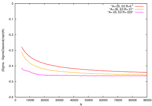
Figure 1: We have plotted $\Delta\sigma_{L}(E_{0},\Delta E)$ (in units of $\kappa_{5}^{2}$) on the $y$-axis which is calculated using (59) and (58). For $N_{n}$, we have used (9) in which the quantity in the RHS is replaced by its nearest integer. $A=\pi\,\Delta ER$. All plots have $E_{0}R\leq 0.25$.

Figure 1 shows that $\Delta\sigma_{L}$ is negative for sufficiently small $E_{0}$ and that for large $N$ the curves behave as $\sqrt{N}$.

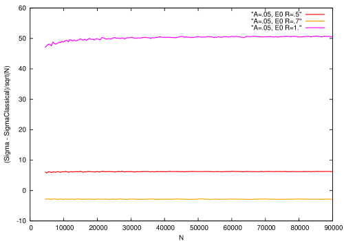
Figure 2: In these plots $E_{0}R\geq.5$. Other things are as in Figure 1.

Figure 2 show that for larger values of $E_{0}$, $\Delta\sigma_{L}$ can be both positive and negative.

Of course, the calculation of the classical cross-section itself is valid for $E_{0}R\ll 1$, together with the other conditions (8)-(14) so perhaps only the first set of plots, $E_{0}R\leq.25$, are relevant.

4.4.5 Atypical states

So far we have only considered typical states with $N_{n}$ given approximately by the thermal distribution.

Let us now briefly consider some states with atypical $N_{n}$. In particular let us suppose that $N$ can be represented as a product $N=p\ q$, where $p,q$ are integers. We will consider

$$N_{n}=p\ \delta_{n,q}$$ (74)

This represents $p$ cycles, each of length $q$.

In this case, (58) simply becomes ($\kappa_{5}^{2}=\kappa^{2}/(VR)$)

$$\Delta\sigma_{L}(E_{0},\Delta E) = 2p\ \kappa_{5}^{2}\ K_{L}(E_{0},\Delta E)\Delta{\tilde{\sigma}}_{L}(q)$$ (75)

Since $\sum_{n}N_{n}=p=N/q$ in this case, the bound on the correction (62) becomes

$$\Delta\sigma_{L,{\rm max}}(E_{0},\Delta E)|_{(p,q)}=\frac{\kappa^{2}}{2VR}\,\frac{N}{q}\tilde{K}_{L}(\frac{E_{0}}{\Delta E})\,L_{L}(\frac{E_{0}}{\Delta E})$$ (76)

Let us consider the two extreme cases:

• Untwisted sector $(p,q)=(N,1)$, i.e. $N_{n}=N\delta_{n,1}$ which implies $N$ short cycles, each of length 1. In this case $\Delta\sigma_{L,{\rm max}}(E_{0},\Delta E)|_{(N,1)}$ in (76) is proportional to $N$ just like the classical answer. An analysis similar to that of Section (4.4.3) then shows that the finite $R$ corrections are now suppressed by a factor of $1/(R\Delta E)$ compared to the classical result.

• Maximally twisted sector $(p,q)=(1,N)$, i.e. $N_{n}=\delta_{n,N}$ which implies one long cycle of length $N$: In this case, $\Delta\sigma_{L,{\rm max}}(E_{0},\Delta E)|_{(1,N)}$ in (76) is independent of $N$ and would be suppressed at least by a power of $1/(NR\Delta E)$.

  In fact, a numerical estimate shows that $\Delta\sigma_{L}$ decays exponentially with $N$. To do the numerical computation, we rewrite (58) for this case as

  $$\Delta\sigma_{L}(E_{0},\Delta E)=\kappa_{5}^{2}\ \frac{N^{2}}{8}\ (R\ \Delta E)^{2}\ \tilde{K}_{L}(E_{0},\Delta E)\ \left(\sum_{m=0}^{\infty}\ f_{L}(m)-\int_{0}^{\infty}\ dx\ f_{L}(x)\right)$$ (77)

  The result is shown for $E_{0}=.01,A=\pi R\ \Delta E=.05$ in Figure 3.

  

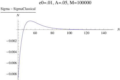
  Figure 3: We show $(\sigma-\sigma_{L,{\rm classical}})/N$ vs $N$ in units $\kappa_{5}^{2}$. $M$ denotes the upper limit in the sum over $m$. $A=\pi R\Delta E,e_{0}=RE_{0}$. The McLaurin upper bound (76) in this case is 0.0278431.

  This is consistent with the behaviour (92) for $E_{0}=0$, viz. $\Delta\sigma_{L}\sim N\,\exp[-N]$.

We have performed numerical calculations also for general $p,q$. From (76), we find that the correction to the classical crosssection vanishes for this case also for $R\Delta E\gg 1$. Numerically, we find that the correction vanishes exponentially with large $q$ and furthermore for values of q beyond a certain value depending on $E_{0}$ and $\Delta E$, the correction changes sign from negative to positive.

4.5 The cross-section for $E_{0}=0$

We now examine the expression (53) for the case $E_{0}=0$. Even though the peak of the wave packet is at zero energy, the spread $\Delta E$ is non-zero, so that the wave packet can sample several energy levels of the system.

If we were to specialize (62) to $E_{0}=0$, we would get (using $\tilde{K}_{L}(0)=2,L(0)=\frac{1}{4}$)

$$\Delta\sigma_{L,{\rm max}}(E_{0}=0,\Delta E)=\frac{\kappa^{2}}{8VR}\sum_{n=1}^{N}N_{n}$$ (78)

For a thermal state, this would become

$$\Delta\sigma_{L,{\rm max}}(E_{0}=0,\Delta E)\approx-\frac{\kappa^{2}}{VR}\,\frac{1}{\beta}\,\left[\log(\beta/2)-\eta\right]$$ (79)

However, for $E_{0}=0$ we can get a better estimate, since the sum in (55) can be performed analytically:

$$\sum_{m=1}^{\infty}\frac{m^{2}}{(m^{2}+a^{2})^{2}}=\frac{\pi}{4a}\left[1+H(2\pi a)\right]$$

where

$$H(x)\equiv\frac{2}{(e^{x}-1)^{2}}\{(1-x)\ e^{x}-1\}=\frac{d}{dx}\,\frac{2x}{e^{x}-1}$$ (80)

It is straightforward to check that $-1\leq H(x)\leq 0$ for $0\leq x\leq\infty$. Therefore the correction is always negative, though the total sum is of course positive.

Using $a=nR\Delta E/2$ we get

$${\tilde{\sigma}}_{L}(n)=\frac{\pi\ R}{32\Delta E}\,n\,\left[1+H(n\,\pi R\Delta E)\right]$$ (81)

The “1” in the square bracket above gives the classical expression

$${\tilde{\sigma}}_{L,{\rm classical}}(n)=\frac{\pi\ R}{32\Delta E}\,n\,$$ (82)

which can be verified by putting $E_{0}=0$ in the expression for ${\tilde{\sigma}}_{L,{\rm classical}}(n)$ in (55). We will see in the next subsection that for typical states the “1” term corresponds to the “continuum limit” $R\gg 1/(\Delta E)$.

Summing over $n$ as in (57), we get

$$\sigma_{L,{\rm classical}}(0,E_{0})=\frac{\pi\kappa^{2}}{8V}(\Delta E)$$

which agrees with the classical answer $\sigma_{\rho,classical}$ from appropriate naive geometry, as in equation (32).

Using (81) and (82) we get

$$\Delta{\tilde{\sigma}}_{L}(n)={\tilde{\sigma}}_{L}(n)-{\tilde{\sigma}}_{L,{\rm classical}}(n)=\frac{\pi\,R}{32\Delta E}\,n\,H(n\,\pi R\Delta E)$$ (83)

Using this in (58) and using $K_{L}(0,\Delta E)=2(\Delta E)^{2}$ we get the following exact expression,

$$\Delta\sigma_{L}(0,\Delta E)=\frac{\pi\kappa^{2}}{8V}(\Delta E)\sum_{n=1}^{N}g(n),\;\;g(n)=n\ N_{n}\ H(\pi nR\Delta E)$$ (84)

As pointed out above $\Delta\sigma_{L}(0,\Delta E)\leq 0$.

4.5.1 $\Delta\sigma$ for a typical state

The microstate dependence is in the above sum over $n$. We will now estimate this sum for a typical microstate at large $N$. As mentioned before, in this case the occupation numbers $N_{n}$ has a thermal distribution given by (9). Therefore the function $g(x)$ in (84) becomes

$$g(x)=x\ H(A\ x)\ \frac{8}{\sinh(\beta x)},\;\beta=\pi\sqrt{\frac{2}{N}},\;A=\pi R(\Delta E)$$ (85)

We now again use the method of Sec. B to obtain the estimate

$$\sum_{n=1}^{N}g(n)=\int_{1}^{N}dx\ g(x)-\eta g(1),\;0<\eta<1,$$ (86)

To find this we have used (119) on the function $-g(x)$ which is positive and monotonically increasing for $x>0$.

Case: $R\ \Delta E\gg 1$

In this case both terms in the RHS behave as $\exp(-\pi R\ \Delta E)$. Hence

$$\Delta\sigma_{L}\sim\exp(-\pi R\ \Delta E)$$ (87)

and the cross-section becomes classical.

Case: $1/\sqrt{N}\ll R\ \Delta E\ll 1$

In order to obtain non-trivial corrections to the classical cross-section from the naive geometry, we therefore must choose $R\ \Delta E\ll 1$. Following the considerations leading to (13) we will in fact estimate the RHS (86) in the regime (13).

It is easy to calculate $g(1)$:

$$g(1)=\frac{1}{\sinh(\beta)}\,\frac{16}{(e^{A}-1)^{2}}\,\{(1-A)e^{A}-1\}\approx\frac{16}{\beta}\ (e^{A}-1)^{-2}\,\{(1-A)e^{A}-1\}$$

For $A\ll 1$, we have

$$g(1)\approx-\frac{8}{\beta}\left(1-\frac{A}{3}+O(A^{3})\right)$$ (88)

The integral over $g(x)$ in (86), unfortunately, cannot be computed exactly. However, in the regime of interest here, it can be approximately evaluated, as follows.

For $A<1,\ 1/A>1$. Note that the function $H(Ax)$ falls off as $\sim\exp[-p]$ beyond $x=p/A>1$. By choosing $p$ sufficiently large we can ignore $g(x)$ beyond this value. Hence we can approximate

$$\int_{1}^{N}dx\ g(x)\approx\int_{1}^{p/A}dx\ g(x)$$

Also in this range $\beta x\ll 1$, hence $x/\sinh(\beta x)\approx 1$. Using these two ingredients, we get

$$\int_{1}^{N}dx\ g(x)\approx\frac{16}{\beta\,A}\,\left[\frac{p}{e^{p}-1}-\frac{A}{e^{A}-1}\right]\approx-\frac{16}{\beta\,A}$$ (89)

In the last step we have used $A\ll 1$ again.

Combining (89) and (88), and using the value of $\beta$, we get the final expression

$$\Delta\sigma_{L}(E_{0}=0,\Delta E)\approx-\sqrt{N}\ \kappa_{5}^{2}\ \frac{\sqrt{2}}{\pi}\;\left[1-\frac{\eta^{\prime}\pi R(\Delta E)}{2}\left(1-\frac{\pi R\Delta E}{3}+O((R\Delta E)^{3})\right)\right]$$ (90)

where in the last step we have used the fact that $\frac{\kappa^{2}}{VR}=\kappa_{5}^{2}$. This is a much more improved estimate compared to (LABEL:smallx). Since for large $N$ we have $\beta\sim 1/{\sqrt{N}}$, the leading term in our regime of interest (13) (which includes $R\Delta E\ll 1$ is now seen to be proportional to $A_{H}$ without any log factor.

We have verified the above conclusions numerically. A sample plot is given in Figure 4.

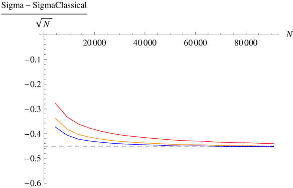
Figure 4: $\Delta\sigma_{L}(0,\Delta E)/\sqrt{N}$ is numerically computed, using (84), and plotted in units of $\kappa_{5}^{2}$ for various values of $A=\pi R\Delta E$. The Red, Orange, Blue and Magenta curves (which go successively down) represent $A=.05,.075,.1$ and .5 respectively. The curves asymptote to constant values ($-\sqrt{2}/\pi\approx-.45$ for small $A$ and increases for larger values of $A$) and are consistent with the analytic estimate (90).

4.5.2 Atypical state

We now evaluate such departures for $E_{0}=0$ in atypical states: which we again take as in (74).

The expression (75) is valid once again, except that we now have an explicit expression for $\Delta{\tilde{\sigma}}_{L}(n)$ in terms of the function $H(\pi\ n\ R\ \Delta E)$, see Eq. (83). With this, we get

$$\Delta\sigma_{L}(E_{0},\Delta E)=\frac{\pi}{8}\ \kappa_{5}^{2}\ (R\Delta E)\,N\ H(q\ A)\ \propto\ N\ H(q\ A)$$ (91)

Here $A=\pi\ R\ \Delta E$.

Thus in the maximally twisted case ($(p,q)=(1,N)$) we have

$$\Delta\sigma_{L}\ \propto\ N\exp[-N]$$ (92)

whereas in the untwisted case ($(p,q)=(N,1)$) we have

$$\Delta\sigma_{L}\ \propto\ N$$

Again, as in the case of general $E_{0}$, the correction is as large as the classical limit.

5 Discussion of Results

The type of corrections to the microscopic cross-section we have calculated in this paper are due to the finite size of the circle on which the D1 branes are wrapped. Note that this is distinct from corrections due to finite $N$. In some cases, e.g. typical states, these corrections are also suppressed by a power of $1/{\sqrt{N}}$. However in other states, e.g. the untwisted sector, these corrections are not suppressed by any power of $N$. In all cases, however, they are suppressed by a power of $1/(R\Delta E)$.

To obtain these corrections one needs to perform two sums: (i) the sum over discrete values of the momenta and (ii) the sum over twists (labelled by $m$ and $n$ respectively in (53)).

For $R\Delta E\gg 1$ the spectrum of the system is practically continuous, and the sum over momenta can be replaced by an integral. Once this is done, the sum over twists is trivial since it appears as $\sum_{n}n\,N_{n}$ which is by definition $N$ see (57). This is why the resulting cross-section is independent of the particular microstate the system is in. The result is also in exact agreement with the semiclassical cross-section obtained in the naive geometry.

The bounds on the corrections to this classical result have been obtained (see Section 4.4) by using McLaurin estimates for the difference between the discrete sums (i) and (ii) and their integral approximants. For $E_{0}=0$ the sum over $m$ may be performed exactly (see Section 4.5), and the McLaurin estimate has been used only for the sum over $n$.

To understand the nature of the sum over $n$ it is useful to consider the case $E_{0}=0$ and consider the contribution ${\tilde{\sigma}}_{L}(n)$ of a given twist sector to the cross-section which is given by (81). In Figure 5 we have plotted $\sigma(n)$ versus $n$, both as histograms for integer $n$ and their continuum approximations where $n$ is replaced by a real number.

1. The upper histogram (and the upper curve which is the continuum approximation) correspond to low resolution (high $R\ \Delta E$). In this case the $H(A\ n)$ term is negligible and this yields the classical limit (82) corresponding to the naive geometry (4).

2. The lower histogram corresponds to high resolution (low $R\ \Delta E$) in which the $H(A\ n)$ term is appreciable. As we have argued in Section 4.4, this histogram, for typical $N_{n}$, can be replaced by its continuum approximation $[8x/\sinh(\beta\ x)]\left(1+H(A\ x)\right)$. Since a typical $N_{n}$ is used, the lower curve represents averaging over the canonical (equivalently, microcanonical) ensemble.

   

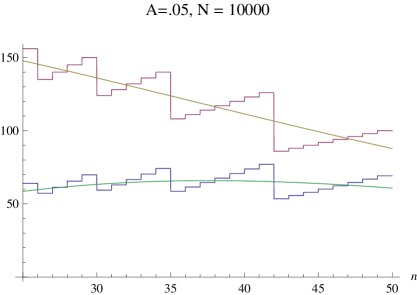
   Figure 5: We have plotted on the $y$-axis ${\tilde{\sigma}}_{L}(n)$ for $E_{0}=0$, in units of $\pi\ R/(32\ \Delta E)$. The upper histogram and curve refer to ${\tilde{\sigma}}_{L,{\rm classical}}(n)$ and its continuum approximation, respectively. In other words the upper histogram corresponds to $n\ [N_{n}]$ where $[\ ]$ represents nearest integer, while the upper curve plots $8x/\sinh(\beta\ x)$. The lower histogram refer to the full expression, $n\ N_{n}\left(1+H(A\ n)\right)$, while the lower curve plots the function $[8x/\sinh(\beta\ x)]\left(1+H(A\ x)\right)$ The upper curve corresponds to the naive geometry which arises due to low resolution (large $A\equiv R\ \Delta E$) while the lower curve refers to a different continuum which arises due to averaging over microstates.

   The second continuum limit, obtained by averaging, yields expressions for $\Delta\sigma_{L}$ of the same form as we obtain in derivative corrected supergravity.

5.1 The Main results

Let us summarize our main results of our computation of corrections explained above:

1. The physically interesting regime (see Eq. (13)) is $1\gg R\Delta E\gg 1/{\sqrt{N}}$. In this regime, the discreteness of the system is manifest but for a typical state there are a large enough number of energy levels in $\Delta E$ to give rise to a time independent absorption cross-section.

   (i) When the central value of the energy $E_{0}$ of the incident wave is much smaller than the width $\Delta E$ we showed that the microstate dependent correction due to discreteness has an upper bound which is independent of all energy scales and proportional to $A_{H}\,\log(N)$ where $A_{H}$ is the area of the stretched horizon. Compared to the microstate independent classical answer, this correction is suppressed by a power of $1/(R\Delta E{\sqrt{N}})$.

   (ii) A better bound has been obtained for $E_{0}=0$, the correction is bounded by simply $A_{H}$ without the $\log(N)$ factor. The sign of the correction is negative. Note, however, that the total cross-section is explicitly positive since it is a sum of positive terms. Of course, in our approximation there is never a domain where the correction is bigger than the classical term.

   (iii) For general small $E_{0}R$, we have numerically calculated the difference between the cross-section and its classical limit for a typical state. The results show that this difference is negative and proportional to $A_{H}$.

   (iv) For larger values of $E_{0}R$ a numerical calculation for the correction yields a positive term proportional to $A_{H}$. However this is not in our regime of interest.

2. We have also obtained estimates for the correction for some atypical states. For the untwisted sector we found that the bound on the finite $R$ correction has the same $N$ dependence as the classical result. The correction is now suppressed by a power of $1/(R\Delta E)$. For the maximally twisted sector, the bound on the correction is independent of $N$. However numerical results of the correction indicate that this is actually suppressed exponentially in $N$ compared to the classical result.

3. The bounds for the correction for a Gaussian profile are similar to those for a Lorentzian profile. In particular, for typical states the bound is proportional to ${\sqrt{N}}$. The proportionality constant becomes a pure number for $E_{0}\ll\Delta E$ and linear in $\frac{E_{0}}{\Delta E}$ for $E_{0}\gg\Delta E$. It is likely that there is a large class of energy profiles for which similar results will hold.

5.2 Appearance of Area of Stretched Horizon

Perhaps the most significant aspect of our results is the fact that for typical states the correction to the naive geometry answer is proportional to the area of the stretched horizon. This is because the results of [8, 9] indicate that higher derivative terms lead to a modification of the geometry near the singular horizon of the naive geometry. The modified geometry has in fact a regular horizon whose area is exactly equal to the area of the stretched horizon of the naive geometry, $A_{H}$.

It is tempting to speculate that the correction term somehow captures this modified geometry with a horizon. We do not have a good understanding of the bulk interpretation of such a correction. The fact that the sign of the correction is negative in most cases we studied numerically, also needs an understanding from the bulk viewpoint, since the general result of [26] would seem to suggest that the zero-frequency limit of the crosssection should be given by the area of the geometry in the higher derivative theory and should hence be a positive quantity . One possible interpretation of our result is that the higher derivative correction to the geometry is equivalent to putting a translucent wall deep down the $AdS_{3}$ throat of the naive geometry. Since such a wall will reflect part of the wave which has entered the $AdS_{3}$ throat, the fraction which would enter this horizon will be less than the fraction of incoming waves at infinity which entered the throat. This would naturally explain why the corrected cross-section is smaller than the classical cross-section, which measures the probability to enter the throat. If this is the case, it is not unlikely that the effect will bring in a factor proportional to the area of the horizon of the effective geometry, assuming such a geometry does indeed arise in our situation due to higher derivative corrections to gravity. This is of course a vague explanation at this point. We hope to form a more concrete picture in the future.

The space-time interpretation of the subleading corrections for atypical states is, however, quite different. A given atypical state corresponds to a specific microstate geometry and the microscopic cross-section corresponds to the probability of entering the throat region. Consider for example the microstates of the type analyzed in sections (4.4.5) and (4.5.2). The bulk descriptions of these microstates have been discussed in Section 3. As shown there, the leading answer for this quantity (in the regime described by (35) simply reproduces the answer in the naive geometry. The calculations in [10] and [30] give an answer valid in a less restrictive regime where the second equation in (35) is not necessary. However since we are interested in finite $R$ corrections, our calculation should be compared to a more refined calculation of scattering of an incoherent beam with a finite energy resolution in such geometries. We defer this calculation for future work.

5.3 Averaging and Horizons

A key feature of our results which is worth emphasizing is that for sufficiently large $R(\Delta E)$, i.e. low energy resolutions, the scattering experiment discussed in this paper perceives the naive geometry for any microstate of the system . The effect of statistical coarse graining over microstates is present in the subleading term. This term certainly does not correspond to scattering in the naive geometry. If anything, this corresponds to a geometry corrected by higher derivative effects. If results similar to [8, 9] hold in this case, the latter geometry has a regular horizon whose Wald entropy agrees with the microscopic entropy.

5.3.1 Comparison with the 3-charge D1-D5-P system

This situation should be contrasted with leading order scattering from a D1-D5-P system with macroscopic amount of momentum in the D1 direction as in [4, 23, 24]. Here the relevant microstates correspond to momentum states of the long string all moving in the same direction (which we will call right moving). Now the probability for absorption is a modification of (42) and (43)

$${\cal P}(E,T)=\sum_{n=1}^{N}N_{n}\,\frac{4\kappa^{2}}{\pi\ V}\frac{1}{ER}\sum_{m=1}^{\infty}(\frac{m}{nR})^{2}\,\rho_{P}(m/nR)\,\left[\frac{\sin(E-\frac{2m}{nR})T}{(E-\frac{2m}{nR})}\right]^{2}$$ (93)

where $\rho_{P}(m/nR)$ is the distribution function of rightmoving momentum among the quanta. This must satisfy

$$\sum_{m=1}^{M}\frac{m}{nR}\rho_{P}(m/nR)=P_{R}$$ (94)

where $P_{R}$ is the total right moving momentum.

In the leading approximation where the discreteness can be ignored, and for long time scales the cross-section then becomes

$$\sigma_{3charge}(E)=\frac{\kappa^{2}E}{4V}\,\sum_{n=1}^{N}\rho_{P}(E/2)nN_{n}$$ (95)

The microstates are now specified by two distribution functions, $N_{n}$ for the twists and $\rho(p)$ for the momenta. The calculations of [4, 23, 24] were performed for a typical state from the point of view of the ensemble defined by $\rho_{P}(p)$. Then $\rho_{P}(p)$ has a thermal form

$$\rho_{P}(p)=\frac{1}{e^{p/T_{R}}-1}$$ (96)

where $T_{R}$ is the right moving temperature which is related to the total momentum $P_{R}$ by requiring (94). Then for $E\ll T_{R}$ one may approximate

$$\rho_{P}(E/2)\sim\frac{2T_{R}}{E}$$ (97)

The factor of $E$ in the denominator then cancels the factor of $E$ in the numerator in (95), and using the fact $T_{R}$ is proportional to the entropy of the system, which in turn is proportional to the horizon area, one gets the result that the cross-section is in fact exactly equal to the horizon area.

Clearly, this result follows only in a typical state. In other words, a statistical averaging over microstates has been performed in addition to coarse-graining due to low resolution of energies to obtain this leading order result.

The key difference between the 2-charge system and the 3-charge system in five dimensions is that the naive geometry of the latter has a smooth large horizon (for large charges). This suggests a connection between statistical averaging and horizons in the type of scattering experiments we have considered in this paper.

5.3.2 Comparison with scattering from massive heterotic BPS states

In [36, 37] scattering of a massless probe, e.g. a graviton, from a massive heterotic BPS state [2] was considered. The “microstate” of the BPS state is given by a polarization tensor $\zeta$. There are many choices of $\zeta$ (called $\zeta_{L}$ in these references), typically of a large rank, which all correspond to a given mass $m$ and charges $\vec{Q}$. The state of the probe is specified by a polarization $\eta$ (of rank 1 or 2). Let us consider for simplicity a process in which the polarizations $\zeta$ and $\eta$ do not change. The structure of the elastic scattering amplitude (at small $\alpha^{\prime}t$) is given by terms such as

$$A(s,t,u) \sim\frac{a}{\alpha^{\prime}t}+b\ \eta_{p}\zeta_{pij..kl}\zeta_{rij..kl}\eta_{r}+O(\alpha^{\prime}t)$$ (98)

$$=\frac{1}{\alpha^{\prime}t}\left(a+b\ \eta_{p}\zeta_{pij..kl}\zeta_{rij..kl}\eta_{r}\ \alpha^{\prime}t+o(\alpha^{\prime}t)^{2}\right)$$

where $a,b$ are numerical factors. In [36] it was shown that the leading term in the small $t$ expansion matched exactly the Rutherford scattering limit of the same probe scattered by the corresponding heterotic black hole [2]. The subleading term, however, has a coupling between the polarization states of the probe and the target BPS state. It was noted in [36] that

1. the low energy term $\sim 1/(\alpha^{\prime}t)$ is independent of the microstate and is reproduced by the “naive” heterotic black hole geometry, and

2. the subleading term depends on the “microstate” and violates the no-hair property.

However, the new point we want to make here is that if we “average” over various “microstates”, denoted in the sum below by a label $q$ stuck to the polarization tensors $\zeta$, the subleading term becomes

$$\sum_{q}\eta_{p}\zeta^{(q)}_{pij..kl}\zeta^{(q)}_{rij..kl}\eta_{r}=\eta_{p}\eta_{r}\delta_{pr}=1$$

leading to a new ‘geometric’ (microstate-independent) expression

$$A(s,t,u)\sim\frac{1}{\alpha^{\prime}t}\left(a+b\alpha^{\prime}t+o(\alpha^{\prime}t)^{2}\right)$$

It may be interesting to note the similarity to the scattering off the 2-charge D1-D5 system we consider in this paper. It is interesting to find out if the microstate-dependent subleading term can be understood in terms of some microstate geometry. It will also be interesting to find out if the geometric expression for the subleading term above corresponds to a finite area horizon which arises out of higher derivative corrections in the supergravity effective action.

6 Concluding Remarks

We have performed a detailed analysis of the microstate dependence of scattering from the D1-D5 system in five dimensions where the internal space is $T^{4}$. The analysis can be extended to the case where the internal manifold is a $K3$. Moreover, microscopic calculations of the absorption cross-sections for a large class of string theory black holes are almost identical to the present case. This suggests that one should perform a similar study for other black holes. In particular the 3-charge system in five dimensions is a straightforward generalization of the 2-charge system (the main formula is given above in (93). Our methods can be easily adapted to this case. It would be interesting to see whether corrections to the classical answer (which again comes from the difference of the expression (93) and its integral approximation) reflect the change of the geometry due to higher derivative supergravity effects. Our considerations can be also directly applied to the 3- and 4- charge systems in four dimensions.

The outstanding open problem here which needs to be addressed in future work is the bulk understanding of our microstate dependent corrections. For typical states, we have offered a very qualitative speculation in this regard, but clearly a lot more work is needed to obtain a precise correspondence. It is also important to understand the relationships of the corrections we have computed for specific microstates to more refined calculations of wave propagation in microstate geometries, as discussed in the previous section.

Finally we emphasize that all our results are in the orbifold limit of the CFT. It is important to find out possible modifications of the result in the presence of deformations.

Acknowledgements

We have benefited from many discussions with Rajiv Bhalerao, Atish Dabholkar, Avinash Dhar, Justin David, K.T. Joseph, Shiraz Minwalla, Ashoke Sen and Spenta Wadia. We are indebted to Samir Mathur for numerous discussions at all stages of this work and for generously sharing his insight. We are grateful to Justin, Samir, Shiraz and Spenta for their comments on the manuscript. We also thank Per Kraus for a correspondence clarifying his work. Much of this work was performed during the Monsoon Workshop on String Theory held at TIFR. We wish to thank International Center for Theoretical Sciences (ICTS), TIFR and the organizers of this workshop for providing an extremely stimulating environment. The work of S.R.D was partially supported by a National Science Foundation Office of International Science and Engineering grant as a part of NSF-PHY-0555444 and by ICTS. Finally we would like to thank the people of India for supporting research in fundamental physics.

Appendix A Absorption cross-section in the naive geometry

Consider the wave equation (23)

$$[(f_{1}f_{5})^{1/2}w^{2}+\frac{1}{r^{3}f_{5}}\partial_{r}(r^{3}f_{5}(f_{1}f_{5})^{-1/2}\partial_{r}]S(r)=0$$ (99)

Far region

The geometry of the far region is flat space-time, and the equation becomes

$$[w^{2}+\frac{1}{r^{3}}\partial_{r}{r^{3}\partial_{r}}]S=0$$ (100)

The solution is

$$S(r)=\frac{1}{\rho}[AJ_{1}(\rho)+BY_{1}(\rho)]$$ (101)

where $\rho=wr$. To avoid complications coming from integer order Bessel functions we will consider in fact the general case where the transverse dimension is $(q+1)$. Then the solution is given by

$$S(r)=\frac{1}{\rho^{\nu}}\left[A\,J_{\nu}(\rho)+B\,J_{-\nu}(\rho)\right]$$ (102)

where $\nu=\frac{1}{2}(q-1)$ is assumed to be non-integral. At $\rho\to\infty$, using the standard asymptotics for Bessel functions we get

$$S(r)\sim\frac{1}{\rho^{\nu+\frac{1}{2}}}\left[C\,e^{i\rho}+D\,e^{-i\rho}\right]$$ (103)

where

$$\frac{C}{D}=e^{-i\frac{\pi}{2}}\frac{1+\frac{B}{A}e^{i\pi\nu}}{1+\frac{B}{A}e^{-i\pi\nu}}$$ (104)

The probability of absorption is then given by

$${\cal P}=1-|\frac{C}{D}|^{2}=\frac{4{\rm Im}\,(\frac{B}{A})\,\sin(\pi\nu)}{1+|\frac{A}{B}|^{2}+\frac{B}{A}e^{-i\pi\nu}+\frac{B^{\star}}{A^{\star}}e^{-i\pi\nu}}$$ (105)

Near region

In the near region, defined in (24), we get the (Poincare patch of the) $AdS_{3}\times S^{3}\times T^{4}$ geometry, and (23) becomes

$$[w^{2}+\frac{r}{\ell^{4}}\partial_{r}{r^{3}\partial_{r}}]S=0$$ (106)

As above, we will consider the generalized case of $AdS_{p+2}\times S^{q}\times T^{4}$ so that the equation becomes

$$[w^{2}+(\frac{\ell}{r})^{p-2}\partial_{r}{(\frac{r}{\ell})^{p+2}\partial_{r}}]S=0$$ (107)

The surface $r=0$ is the “Poincare horizon”. We will consider solutions which are ingoing at $r=0$. This is given by

$$S(r)=E\,(\frac{w\ell^{2}}{r})^{\mu}\,H^{(1)}_{\mu}(\frac{w\ell^{2}}{r})~{}~{}~{}~{}~{}~{}~{}~{}~{}~{}\mu=\frac{p+1}{2}$$ (108)

In the limit $r\rightarrow 0$ this solution behaves as

$$S\rightarrow e^{i\frac{w\ell^{2}}{r}}$$ (109)

Intermediate Region

In the intermediate region, we have to use the large $r$ behavior of (108) and the small $r$ behavior of (102) and match the two solutions. The small $r$ behavior of (102) is

$$S\sim\frac{A}{2^{\nu}\,\Gamma(1+\nu)}+\frac{B\,2^{\nu}}{\rho^{2\nu}\,\Gamma(1-\nu)}$$ (110)

while the large $r$ behavior of (108) is

$$S\sim\frac{iE}{\sin(\pi\mu)}\left[\frac{(w\ell^{2})^{2\mu}\,e^{-i\pi\mu}}{r^{2\mu}\,2^{\mu}\,\Gamma(1+\mu)}-\frac{2^{\mu}}{\Gamma(1-\mu)}\right]$$ (111)

Matching and Cross-section

The expressions (111) and (110) can be matched if $\mu=\nu$, i.e. $q=p+2$. For our present case $p=1$, so that $\mu=\nu=1$. However, we will retain a general $\mu,\nu$. Matching then yields

$$\frac{B}{A}=-\frac{e^{-i\pi\mu}}{2^{4\mu}\,[\Gamma(1+\mu)]^{2}}\,[\Gamma(1-\nu)]^{2}\,(w\ell)^{4\mu}$$ (112)

Using $\mu=\nu$ this give the following expression for the probability of absorption (105)

$${\cal P}=\frac{4\pi^{2}}{[\Gamma(\mu)]^{2}}\frac{(w\ell)^{4\mu}}{2^{4\mu}\,[\Gamma(1+\mu)]^{2}}$$ (113)

The cross-section $\sigma_{cl}$ is obtained by multiplying this quantity by the fraction of a spherical wave which is in a plane wave. For a $q+1$ dimensional transverse space this gives

$$\sigma_{cl}={\cal P}\,(4\pi)^{\frac{q-1}{2}}\,\Gamma(\frac{q+1}{2})\frac{1}{w^{q}}$$ (114)

Substituting (113) we finally get

$$\sigma_{cl}=\frac{4\pi^{2}(4\pi)^{\mu}}{[\Gamma(\mu)\Gamma(1+\mu)]^{2}\frac{\Gamma(1+\mu)}{2^{4\mu}}w^{2\mu-1}\,\ell^{4\mu}}$$ (115)

For our present case, $\mu=\nu=1$ yields

$$\sigma_{cl}=\pi^{3}\ell^{4}\,w$$ (116)

which is (26).

Appendix B McLaurin integral approximation for sums

The McLaurin integral approximation states that if a function $f_{L}(x)$ is positive and monotonically decreasing in $P\leq x\leq Q$, the following is true

$$\int_{P}^{Q}dx\ f_{L}(x)+f_{L}(P)>\sum_{n=P}^{Q}f_{L}(i)>\int_{P}^{Q}dx\ f_{L}(x)+f_{L}(Q),$$ (117)

We can rewrite the above in the form of an estimate for the sum:

$$\sum_{n=P}^{Q}f_{L}(i)=\int_{P}^{Q}dx\ f_{L}(x)+f_{L}(Q)+\eta_{1}\left(f_{L}(P)-f_{L}(Q)\right),\;0<\eta_{1}<1$$ (118)

Similarly, for a positive monotonically increasing function $f_{L}(x)$ in $P^{\prime}\leq x\leq Q^{\prime}$, we get

$$\sum_{n=P^{\prime}}^{Q^{\prime}}f_{L}(i)=\int_{P^{\prime}}^{Q^{\prime}}dx\ f_{L}(x)+f_{L}(P^{\prime})+\eta_{2}\left(f_{L}(Q^{\prime})-f_{L}(P^{\prime})\right),\;0<\eta_{2}<1$$ (119)

Using these two results we can find integral estimates for sums, for any function $f_{L}(x)$ with a finite number of minima and maxima, as we will do now.

B.1 Details of estimation of $\Delta{\tilde{\sigma}}_{L}(n)$

We will use the notation

$$I(P,Q)=\int_{P}^{Q}dx\,f_{L}(x),S(P,Q)=\sum_{m=P}^{Q}f_{L}(m).$$

Let us apply the McLaurin integral estimates above to (59) which we rewrite as

$$\Delta{\tilde{\sigma}}_{L}(n)=\frac{(nR)^{2}}{16}[S(0,\infty)-I(0,\infty)]$$ (120)

In $0<x<\infty$ the function $f_{L}(x)$ is positive and has one extremum, viz. a maximum at

$$x_{1}=\sqrt{a^{2}+b^{2}}$$ (121)

Thus, $f_{L}(x)$ is monotonically increasing in the segment $x\in(0,x_{1})$ and monotonically decreasing in the segment $x\in(x_{1},\infty)$.

In segment $(0,n_{1})\subset(0,x_{1})$ we use (119) and obtain

$$S(0,n_{1})=I(0,n_{1})+\eta_{1}\,f_{L}(n_{1}),\;0<\eta_{1}<1$$ (122)

Here $n_{1}=\lfloor x_{1}\rfloor$ denotes the integer part of $x_{1}$.

In segment $(n_{1}+1,\infty)\subset(x_{1},\infty)$ we use (118) and have (using $f_{L}(\infty)\to 0$)

$$S(n_{1}+1,\infty)=I(n_{1}+1,\infty)+\eta_{2}\,f_{L}(n_{1}+1),\;0<\eta_{2}<1$$ (123)

Combining the last two equations, we get

$$S(0,\infty)=I(0,\infty)-I(n_{1},n_{1}+1)+\eta_{1}\,f_{L}(n_{1})+\eta_{2}\,f_{L}(n_{1}+1)$$ (124)

We can approximate $I(n_{1},n_{1}+1)\approx f_{L}(n_{1})\approx f_{L}(n_{1}+1)\approx f_{L}(x_{1})$. Thus,

$$S(0,\infty)-I(0,\infty)\approx f_{L}(x_{1})\ \eta_{3},\;\;\eta_{3}=\eta_{1}+\eta_{2}-1\in(-1,1)$$ (125)

By using this in (120), and the value

$$f_{L}(x_{1})=\frac{b^{2}+a^{2}}{(a^{2}+(\sqrt{b^{2}+a^{2}}-b)^{2})^{2}},$$ (126)

with $(a,b)$ as in (56), we obtain

$$\Delta{\tilde{\sigma}}_{L}(n)\approx\eta_{3}(n)\frac{1}{4}\frac{E_{0}^{2}+{\Delta E}^{2}}{({\Delta E}^{2}+(\sqrt{E_{0}^{2}+{\Delta E}^{2}}-E_{0})^{2})^{2}}$$ (127)

We have displayed the possible dependence of the fraction $\eta_{3}$ on $a,b$ and hence on $n$.

Appendix C Results for a Gaussian Profile

In this section we give the results for the upper bound on the correction to the cross-section when we use a Gaussian profile of the form given in (17).

In this case, the absorption cross-section $\sigma_{L}(E_{0},\Delta E)$ becomes, instead of (53),

$$\sigma_{G}(E_{0},\Delta E) = \frac{2\kappa^{2}}{VR}\,K_{G}(E_{0},\Delta E)\,\sum_{n=1}^{N}N_{n}{\tilde{\sigma}}_{G}(n),$$

$${\tilde{\sigma}}_{G}(n) \equiv \sum_{m=1}^{\infty}(\frac{m}{nR})^{2}{\rm exp}\left[-\frac{(\frac{2m}{nR}-E_{0})^{2}}{(\Delta E)^{2}}\right]$$ (128)

where the function $K_{G}(x)$ is the normalization defined in (16) for the Gaussian profile

$$K_{G}(E_{0},\Delta E)=\frac{2}{(\Delta E)^{2}}~{}\tilde{K}_{G}(E_{0}/\Delta E)$$ (129)

and $\tilde{K}_{G}(x)$ has been defined in (21). When the sum over $m$ is replaced by an integral we once again recover the classical answer (29), exactly as in equation (55)-(57). The function which appears in the integral is now $f_{G}(x)$ (instead of $f_{L}(x)$ of (56)),

$$f_{G}(x)=x^{2}~{}{\rm exp}\left[-\frac{(x-b)^{2}}{a^{2}}\right]$$ (130)

where $a$ and $b$ are defined in (56).

The departure from the classical limit is now given by

$$\Delta\sigma_{G}(E_{0},\Delta E) = \sigma_{G}(E_{0},\Delta E)-{\sigma}_{G,\rm classical}(E_{0},\Delta E)$$ (131)

$$= \frac{2\kappa^{2}}{VR}\,K_{G}(E_{0},\Delta E)\,\sum_{n=1}^{N}N_{n}\Delta{\tilde{\sigma}}_{G}(n)$$

where

$$\Delta{\tilde{\sigma}}_{G}(n)\equiv{\tilde{\sigma}}_{G}(n)-{\tilde{\sigma}}_{G,{\rm classical}}(n)=\frac{1}{(nR)^{2}}\left(\sum_{m=0}^{\infty}f_{G}(m)-\int_{0}^{\infty}\ dx\ f_{G}(x)\right)$$ (132)

The function $f_{G}(x)$ is quite similar to $f_{L}(x)$. In $0<x<\infty$ this is positive with a single maximum at $x=x_{2}$,

$$x_{2}=\frac{1}{2}\left[b+{\sqrt{b^{2}+4a^{2}}}\right]$$ (133)

The arguments of section (B) then show that an upper bound for $\Delta{\tilde{\sigma}}_{G}(n)$ is given in terms of $f_{G}(x_{2})$, exactly as in (125). This leads to

$$\Delta{\tilde{\sigma}}_{G}(n)\approx\frac{\eta_{4}(n)}{4}(\Delta E)^{2}\left[\left(\frac{E_{0}}{\Delta E}+{\sqrt{4+\frac{E_{0}^{2}}{(\Delta E)^{2}}}}\right)^{2}~{}{\rm exp}\{-\frac{1}{4}\left({\sqrt{4+\frac{E_{0}^{2}}{(\Delta E)^{2}}}}-\frac{E_{0}}{\Delta E}\right)^{2}\}\right]$$ (134)

where $-1<\eta_{4}(n)<1$. Exactly as in (60), the factors of $(nR)$ have cancelled and the only $n$ dependence is in $\eta_{4}(n)$. Furthermore, the factor of $(\Delta E)^{2}$ in (134) cancels an overall factor of $1/(\Delta E)^{2}$ present in $K_{G}(E_{0},\Delta E)$ in (129) leading to the final bound, which is the analog of (62),

$$\Delta\sigma_{G,{\rm max}}(E_{0},\Delta E)=\frac{4\kappa^{2}}{VR}\,\tilde{K}_{G}(\frac{E_{0}}{\Delta E})\,L_{G}(\frac{E_{0}}{\Delta E})\,\sum_{n=1}^{N}N_{n}$$ (135)

where the function $L_{G}(x)$ is defined in (21).

As in the case of a Lorentzian profile, the microstate dependence of this bound is entirely in the sum $\sum_{m=1}^{N}N_{n}$. For a typical state this sum can be estimated as in (65). This leads to the final expression for the bound in (20).

For $E_{0}\ll\Delta E$, we have the expansion

$$\tilde{K}_{G}(\frac{E_{0}}{\Delta E})\,L_{G}(\frac{E_{0}}{\Delta E})=\frac{4}{e}[1+(2-\sqrt{\pi})\frac{E_{0}}{\Delta E}+\cdots]$$ (136)

This means that for typical states we have

$$\Delta\sigma_{G,{\rm max}}(E_{0},\Delta E)|_{E_{0}\ll\Delta E}\propto A_{H}$$ (137)

just like the Lorentzian profile result (70). For $E_{0}\gg\Delta E$

$${\tilde{K}}_{G}(x)\sim\frac{1}{x}~{}~{}~{}~{}~{}~{}~{}~{}~{}L_{G}(x)\sim x^{2}$$ (138)

so that

$$\Delta\sigma_{G,{\rm max}}(E_{0},\Delta E)|_{E_{0}\gg\Delta E}\propto A_{H}~{}\frac{E_{0}}{\Delta E}$$ (139)

similar to (73).

References

- [1] A. Dabholkar and J. A. Harvey, “Nonrenormalization of the Superstring Tension,” Phys. Rev. Lett. 63, 478 (1989); A. Dabholkar, G. W. Gibbons, J. A. Harvey and F. Ruiz Ruiz, “SUPERSTRINGS AND SOLITONS,” Nucl. Phys. B 340, 33 (1990).
- [2] A. Sen, “Extremal black holes and elementary string states,” Mod. Phys. Lett. A 10, 2081 (1995) [arXiv:hep-th/9504147]. A. Sen, “Black holes and elementary string states in N = 2 supersymmetric string theories,” JHEP 9802, 011 (1998) [arXiv:hep-th/9712150].
- [3] A. Strominger and C. Vafa, “Microscopic Origin of the Bekenstein-Hawking Entropy,” Phys. Lett. B 379, 99 (1996) [arXiv:hep-th/9601029];
- [4] C. G. Callan and J. M. Maldacena, “D-brane Approach to Black Hole Quantum Mechanics,” Nucl. Phys. B 472, 591 (1996) [arXiv:hep-th/9602043].
- [5] J. de Boer, “Six-dimensional supergravity on S**3 x AdS(3) and 2d conformal field theory,” Nucl. Phys. B 548, 139 (1999) [arXiv:hep-th/9806104]; N. Seiberg and E. Witten, “The D1/D5 system and singular CFT,” JHEP 9904, 017 (1999) [arXiv:hep-th/9903224]; F. Larsen and E. J. Martinec, “U(1) charges and moduli in the D1-D5 system,” JHEP 9906, 019 (1999) [arXiv:hep-th/9905064].
- [6] J. R. David, G. Mandal and S. R. Wadia, “Microscopic formulation of black holes in string theory,” Phys. Rept. 369, 549 (2002) [arXiv:hep-th/0203048].
- [7] For a compact review, see Appendix A of [18].
- [8] A. Dabholkar, “Exact counting of black hole microstates,” Phys. Rev. Lett. 94, 241301 (2005) [arXiv:hep-th/0409148]; A. Dabholkar, R. Kallosh and A. Maloney, “A stringy cloak for a classical singularity,” JHEP 0412, 059 (2004) [arXiv:hep-th/0410076]; V. Hubeny, A. Maloney and M. Rangamani, “String-corrected black holes,” JHEP 0505, 035 (2005) [arXiv:hep-th/0411272]; A. Dabholkar, F. Denef, G. W. Moore and B. Pioline, “Precision counting of small black holes,” JHEP 0510, 096 (2005) [arXiv:hep-th/0507014]; V. Hubeny, A. Maloney and M. Rangamani, “String-corrected black holes,” JHEP 0505, 035 (2005) [arXiv:hep-th/0411272].
- [9] A. Castro, J. L. Davis, P. Kraus and F. Larsen, “5D attractors with higher derivatives,” JHEP 0704, 091 (2007) [arXiv:hep-th/0702072]. A. Castro, J. L. Davis, P. Kraus and F. Larsen, “5D Black Holes and Strings with Higher Derivatives,” JHEP 0706, 007 (2007) [arXiv:hep-th/0703087]. A. Castro, J. L. Davis, P. Kraus and F. Larsen, “String Theory Effects on Five-Dimensional Black Hole Physics,” arXiv:0801.1863 [hep-th]. A. Castro, J. L. Davis, P. Kraus and F. Larsen, “Precision entropy of spinning black holes,” JHEP 0709, 003 (2007) [arXiv:0705.1847 [hep-th]].
- [10] O. Lunin and S. D. Mathur, “The slowly rotating near extremal D1-D5 system as a ’hot tube’,” Nucl. Phys. B 615, 285 (2001) [arXiv:hep-th/0107113]
- [11] O. Lunin and S. D. Mathur, “AdS/CFT duality and the black hole information paradox,” Nucl. Phys. B 623, 342 (2002) [arXiv:hep-th/0109154]; For reviews and references to the extensive original literature in this field see S. D. Mathur, “The fuzzball proposal for black holes: An elementary review,” Fortsch. Phys. 53, 793 (2005) [arXiv:hep-th/0502050]; S. D. Mathur, “What Exactly is the Information Paradox?,” arXiv:0803.2030 [hep-th]; CITATION = FPYKA,53,793;K. Skenderis and M. Taylor, “The fuzzball proposal for black holes,” arXiv:0804.0552 [hep-th].
- [12] For a review and references to the original literature see I. Bena and N. P. Warner, “Black holes, black rings and their microstates,” Lect. Notes Phys. 755, 1 (2008) [arXiv:hep-th/0701216].
- [13] S. Corley, A. Jevicki and S. Ramgoolam, “Exact correlators of giant gravitons from dual N = 4 SYM theory,” Adv. Theor. Math. Phys. 5, 809 (2002) [arXiv:hep-th/0111222]; D. Berenstein, “A toy model for the AdS/CFT correspondence,” JHEP 0407, 018 (2004) [arXiv:hep-th/0403110]; H. Lin, O. Lunin and J. M. Maldacena, “Bubbling AdS space and 1/2 BPS geometries,” JHEP 0410, 025 (2004) [arXiv:hep-th/0409174];
- [14] V. Balasubramanian, V. Jejjala and J. Simon, “The library of Babel,” Int. J. Mod. Phys. D 14, 2181 (2005) [arXiv:hep-th/0505123]. V. Balasubramanian, J. de Boer, V. Jejjala and J. Simon, “The library of Babel: On the origin of gravitational thermodynamics,” JHEP 0512, 006 (2005) [arXiv:hep-th/0508023].
- [15] S. J. Rey and Y. Hikida, “Black hole as emergent holographic geometry of weakly interacting hot Yang-Mills gas,” JHEP 0608, 051 (2006) [arXiv:hep-th/0507082]; D. Berenstein, “Large N BPS states and emergent quantum gravity,” JHEP 0601, 125 (2006) [arXiv:hep-th/0507203]; P. G. Shepard, “Black hole statistics from holography,” JHEP 0510, 072 (2005) [arXiv:hep-th/0507260];
- [16] N. V. Suryanarayana, “Half-BPS giants, free fermions and microstates of superstars,” JHEP 0601, 082 (2006) [arXiv:hep-th/0411145].
- [17] G. Mandal, “Fermions from half-BPS supergravity,” JHEP 0508, 052 (2005) [arXiv:hep-th/0502104]. A. Dhar, G. Mandal and N. V. Suryanarayana, “Exact operator bosonization of finite number of fermions in one space dimension,” JHEP 0601, 118 (2006) [arXiv:hep-th/0509164].
- [18] V. Balasubramanian, P. Kraus and M. Shigemori, “Massless black holes and black rings as effective geometries of the D1-D5 system,” Class. Quant. Grav. 22, 4803 (2005) [arXiv:hep-th/0508110].
- [19] V. Balasubramanian, B. Czech, V. E. Hubeny, K. Larjo, M. Rangamani and J. Simon, “Typicality versus thermality: An analytic distinction,” arXiv:hep-th/0701122; S. J. Rey and Y. Hikida, “Emergent AdS(3) and BTZ black hole from weakly interacting hot 2d CFT,” JHEP 0607, 023 (2006) [arXiv:hep-th/0604102]. L. F. Alday, J. de Boer and I. Messamah, “The gravitational description of coarse grained microstates,” JHEP 0612, 063 (2006) [arXiv:hep-th/0607222].
- [20] V. S. Rychkov, “D1-D5 black hole microstate counting from supergravity,” JHEP 0601, 063 (2006) [arXiv:hep-th/0512053].
- [21] A. Donos and A. Jevicki, “Dynamics of chiral primaries in AdS(3) x S**3 x T**4,” Phys. Rev. D 73, 085010 (2006) [arXiv:hep-th/0512017].
- [22] L. Schiff, ”Quantum Mechanics”, 3rd Edition, McGraw-Hill International Edition, pp 401-403.
- [23] A. Dhar, G. Mandal and S. R. Wadia, “Absorption vs decay of black holes in string theory and T-symmetry,” Phys. Lett. B 388, 51 (1996) [arXiv:hep-th/9605234].
- [24] S. R. Das and S. D. Mathur, “Comparing decay rates for black holes and D-branes,” Nucl. Phys. B 478, 561 (1996) [arXiv:hep-th/9606185]; S. R. Das and S. D. Mathur, “Interactions involving D-branes,” Nucl. Phys. B 482, 153 (1996) [arXiv:hep-th/9607149].
- [25] J. M. Maldacena and A. Strominger, “Black hole greybody factors and D-brane spectroscopy,” Phys. Rev. D 55, 861 (1997) [arXiv:hep-th/9609026].
- [26] S. R. Das, G. W. Gibbons and S. D. Mathur, “Universality of low energy absorption cross sections for black holes,” Phys. Rev. Lett. 78, 417 (1997) [arXiv:hep-th/9609052].
- [27] R. Emparan, “Absorption of scalars by extended objects,” Nucl. Phys. B 516, 297 (1998) [arXiv:hep-th/9706204].
- [28] J. M. Maldacena, “D-branes and near extremal black holes at low energies,” Phys. Rev. D 55, 7645 (1997) [arXiv:hep-th/9611125]; S. R. Das, “The effectiveness of D-branes in the description of near-extremal black holes,” Phys. Rev. D 56, 3582 (1997) [arXiv:hep-th/9703146]; J. R. David, G. Mandal and S. R. Wadia, “Microscopic formulation of black holes in string theory,” Phys. Rept. 369, 549 (2002) [arXiv:hep-th/0203048].
- [29] G. Baym, ”Lectures on Quantum Mechanics”, Westview Press (1974).
- [30] S. Giusto, S. D. Mathur and A. Saxena, “3-charge geometries and their CFT duals,” Nucl. Phys. B 710, 425 (2005) [arXiv:hep-th/0406103].
- [31] S. D. Mathur, “The fuzzball proposal for black holes: An elementary review,” Fortsch. Phys. 53, 793 (2005) [arXiv:hep-th/0502050].
- [32] D. N. Page, “Particle Emission Rates From A Black Hole: Massless Particles From An Uncharged, Nonrotating Hole,” Phys. Rev. D 13, 198 (1976); W. G. Unruh, “Absorption Cross-Section Of Small Black Holes,” Phys. Rev. D 14, 3251 (1976).
- [33] V. Balasubramanian, J. de Boer, E. Keski-Vakkuri and S. F. Ross, “Supersymmetric conical defects: Towards a string theoretic description of black hole formation,” Phys. Rev. D 64, 064011 (2001) [arXiv:hep-th/0011217].
- [34] J. M. Maldacena and L. Maoz, “De-singularization by rotation,” JHEP 0212, 055 (2002) [arXiv:hep-th/0012025].
- [35] J. R. David, G. Mandal and S. R. Wadia, “Absorption and Hawking radiation of minimal and fixed scalars, and AdS/CFT correspondence,” Nucl. Phys. B 544, 590 (1999) [arXiv:hep-th/9808168].
- [36] G. Mandal and S. R. Wadia, “Black Hole Geometry around an Elementary BPS String State,” Phys. Lett. B 372, 34 (1996) [arXiv:hep-th/9511218].
- [37] J. R. David, A. Dhar, G. Mandal and S. R. Wadia, “Observability of quantum state of black hole,” Phys. Lett. B 392, 39 (1997) [arXiv:hep-th/9610120].
- [38] F. Moura and R. Schiappa, “Higher-derivative corrected black holes: Perturbative stability and absorption cross-section in heterotic string theory,” Class. Quant. Grav. 24, 361 (2007) [arXiv:hep-th/0605001].