Rare Muon Decay $\mu^{+}\to e^{+}e^{-}e^{+}\nu_{e}\bar{\nu_{\mu}}$

Abstract

An analytical expression for the spin-averaged amplitude squared of the rare muon decay $\mu^{+}\to e^{+}e^{-}e^{+}\nu_{e}\bar{\nu_{\mu}}$ is calculated. Monte Carlo phase space simulation using the analytical expression for the amplitude has been used to get various differential distributions of charged leptons. The approximate analytical expression for the total energy spectrum of charged leptons near the end point is presented. The dependence of branching ratio on cuts in total energy of charged leptons is studied taking into account an experimental energy resolution. It is shown that the measured branching ratio is very sensitive to the energy resolution.

The observation of lepton flavor violation (LFV) processes would indicate new physics beyond the Standard Model [1], [2]. The lepton flavor violation effects in processes of $\mu\to e$ conversion in a muonic atom, radiative muon decay $\mu^{+}\to e^{+}\gamma$ and muon decay $\mu^{+}\to e^{+}e^{-}e^{+}$ may be large enough to be detected in the future experiments. Ideas [3] of improvement of muon beam intensity by a few orders of magnitude lead to new possibilities in designing of new lepton flavor violation experiments. Analysis of rare background processes is very important for understanding the feasibility of such experiments.

In this article we consider the process

$$\mu^{+}\to e^{+}e^{-}e^{+}\nu_{e}\bar{\nu_{\mu}}$$ (1)

which is the most important background process in searches for the lepton flavor violating muon decay $\mu^{+}\to e^{+}e^{-}e^{+}$. The current measured branching ratio for process (1) is $\Gamma(\mu^{+}\to e^{+}e^{-}e^{+}\nu_{e}\bar{\nu_{\mu}})/\Gamma_{total}=(3.4\pm 0.4)\times 10^{-5}$   [4],[5].

The detailed analysis of background processes for new experiments searching for the muon decay $\mu^{+}\to e^{+}e^{-}e^{+}$ requires knowledge of the amplitude of process (1).

The branching ratio of process (1) was first calculated in [6] and [7] and later in [8], [9] and [10]. Unfortunately works [6] and [8] were not published, and articles [7] and [9] give only final results of calculations for specific experimental cuts or without cuts. In [10] the analysis of process (1) was performed but the final expression for the squared amplitude was not given.

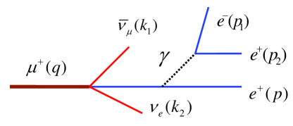
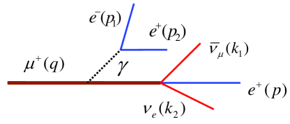
Figure 1: Two Feynman diagrams for the process (1). The other two diagrams are obtained by the interchange $p\leftrightarrow p_{2}$.

In order to allow calculation of the branching ratio of process (1) for any desired cuts and parameters an analytical expression for spin-averaged amplitude squared $\overline{|\tilde{F}|^{2}}$ is presented in the Appendix. The amplitude was calculated for the case of a V-A interaction and unpolarized muons by using Mathematica 6.0 and FeynCalc 6.0.0 [11]. The branching ratio calculation of process (1) combines $\overline{|\tilde{F}|^{2}}$ with a phase space Monte Carlo simulation. In comparison with the previous articles (such as [9] using the $1.3\times 10^{6}$ events) the statistics was significantly increased to $10^{8}$ and $5\times 10^{8}$ events in dependence on cuts applied to charged lepton energies.

In the lowest order in perturbation theory process (1) is described by four Feynman diagrams, two of which are shown in Fig.1. The other two are obtained by the interchange $p\leftrightarrow p_{2}$. Additional diagrams corresponding to particle emission from internal W-boson lines are suppressed by a factor $\sim(m_{\mu}/M_{W})^{2}\sim 10^{-6}$.

Below we present the results of these calculations of the branching ratio

$$R\equiv\frac{\Gamma(\mu^{+}\to e^{+}e^{-}e^{+}\nu_{e}\bar{\nu_{\mu}})}{\Gamma(\mu^{+}\to e^{+}\nu_{e}\bar{\nu_{\mu}})}$$ (2)

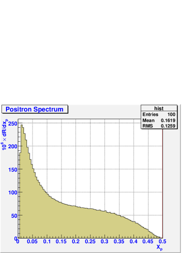
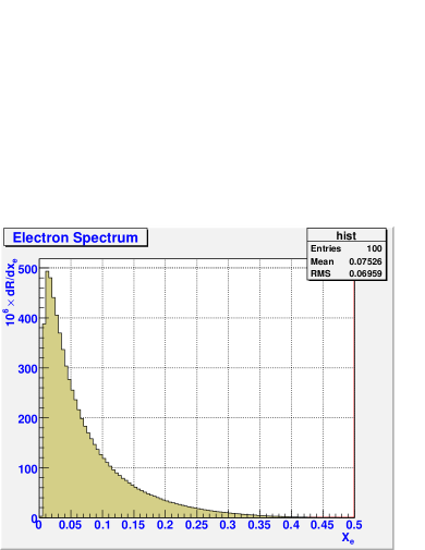
Figure 2: The distribution in positron energy $dR/dx_{p}$ (left) and the distribution in electron energy $dR/dx_{e}$ (right) where $x_{p}=E_{p}/m_{\mu}$ and $x_{e}=E_{e}/m_{\mu}$

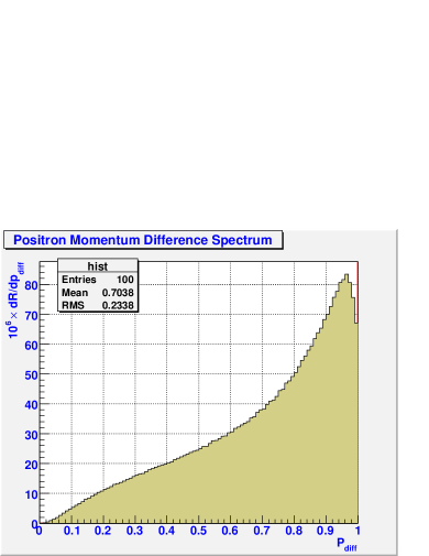
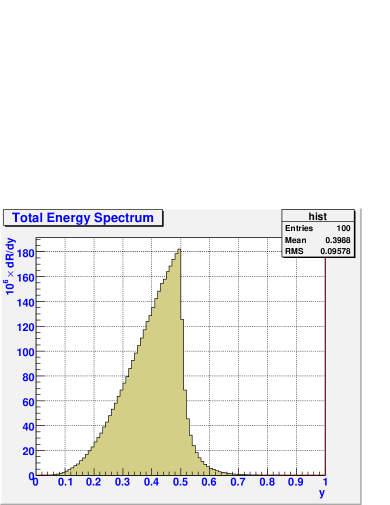
Figure 3: The distribution in positron variable $dR/dp_{diff}$ (left) and the distribution in total energy of charged leptons (right) where $y=E_{tot}/m_{\mu}$.

Distributions in positron energy and electron energy without cuts for process (1) are shown in Fig.2. The positron distribution is characterized by a long tail up to the maximum positron energy. The electron distribution peaks near zero and decreases quickly as electron energy tends to its upper limit.

The distribution in relative positron momentum difference $p_{diff}\equiv|\overrightarrow{p}-\overrightarrow{p_{2}}|/|\overrightarrow{p}+\overrightarrow{p_{2}}|$ where $p$ and $p_{2}$ are positron momenta is shown in Fig.3 (left). The $p_{diff}$ distribution vanishes at $p_{diff}=0$ in agreement with Fermi statistics of positrons. A distribution in total energy $E_{tot}$ of all charged leptons without cuts is shown in Fig.3 (right). The spectrum is steep in the region above $0.5m_{\mu}$. This is important for background suppression in searches for lepton flavor violating process $\mu^{+}\to e^{+}e^{-}e^{+}$.

Cut $(m_{\mu}-E_{tot})$	Statistics	Branching ratio R
$1m_{e}$	$5\times 10^{8}$	$(2.83\pm 0.16)\times 10^{-19}$
$5m_{e}$	$5\times 10^{8}$	$(4.660\pm 0.046)\times 10^{-15}$
$10m_{e}$	$10^{8}$	$(3.091\pm 0.032)\times 10^{-13}$
$50m_{e}$	$10^{8}$	$(7.127\pm 0.013)\times 10^{-9}$
$100m_{e}$	$10^{8}$	$(2.1123\pm 0.0022)\times 10^{-6}$
no cut	$10^{8}$	$(3.5908\pm 0.0033)\times 10^{-5}$

Table 1: The branching ratio R versus cut $(m_{\mu}-E_{tot})$ on the total energy of charged leptons. The cut is measured in the electron mass $m_{e}$.

The results of calculations of the branching ratio R are presented in Table 1 and Fig.4 (right) versus cut on $(m_{\mu}-E_{tot})$ where $E_{tot}$ is the total energy of all charged leptons. Without cuts our result is in agreement with the results of articles [7], [9] and [10]: $R=(3.54\pm 0.09)\times 10^{-5}$, $R=(3.5916\pm 0.0022)\times 10^{-5}$ and $R=(3.6\pm 0.1)\times 10^{-5}$ respectively. For the cut $(m_{\mu}-E_{tot})=5m_{e}$ our result is close to those of [9] but for cuts of 10, 50, 100$m_{e}$ our results are less by a factor 10. We note that the differential distribution $dR/dE_{tot}$ of [9] contradicts the results quoted in their table.

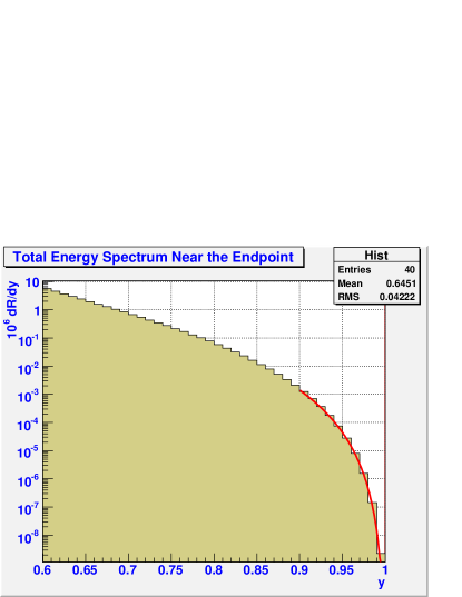
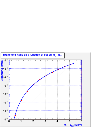
Figure 4: The total energy spectrum dR/dy near the endpoint (left) and the branching ratio R versus cut on the total energy of charged leptons (right) where $y=E_{tot}/m_{\mu}$. Smooth lines show the results of fit.

Also, we would like to note that uncertainties in [9] appear quite small for the given number of trials. Our statistics is about 100 times higher but uncertainties are comparable with [9].

Note that the cut $<5m_{e}$ (see first lines in Table 1) corresponds to the region of interest in searches for the lepton flavor violating process $\mu^{+}\to e^{+}e^{-}e^{+}$. By applying fit to the region near the endpoint (see Fig.4(left)) an approximate expression for the spectrum in this region was found to be

$$dR/dy=C\cdot(1-y)^{5}$$ (3)

where $C=1.4\times 10^{-4}$ and $y=E_{tot}/m_{\mu}$.

Fit of the branching ratio R (see Fig.4(right)) near the endpoint gives an approximate expression

$$R=2.99\cdot 10^{-19}~{}\big{(}\frac{m_{\mu}-E_{tot}}{m_{e}}\big{)}^{6}$$ (4)

Below we show that the steep behavior of the total energy spectrum near the endpoint with a finite detector resolution lead to a significant increase in the number of background events of type (1) in searches for lepton flavor violating muon decay $\mu^{+}\to e^{+}e^{-}e^{+}$.

The branching ratio to have a signal from muon decay (1) above a threshold $m_{\mu}-\Delta$ is given by

$$R_{exp}=\int\limits_{m_{\mu}-\Delta}^{\infty}dE^{m}_{tot}\int\limits_{0}^{m_{\mu}}dR/dE_{tot}\cdot f(E^{m}_{tot}-E_{tot})dE_{tot}$$ (5)

where $E^{m}_{tot}$ is the measured total energy of charged particles, $E_{tot}$ is the true total energy, $\Delta$ is a value measured from the total energy endpoint, $dR/dE_{tot}$ is the total energy spectrum near the endpoint, and f is the resolution function of the detector.

For the detector response function of the Gaussian form $f(x)=\frac{1}{\sqrt{2\pi}\cdot\sigma}~{}~{}exp(~{}-\frac{x^{2}}{2\sigma^{2}}~{})$ the branching ratio $R_{exp}$, given by Eq.(5), can be calculated analytically by using expression (3) for the total energy spectrum. In this case

$$R_{exp}=\frac{C}{6\sqrt{2\pi}}~{}(\frac{\sigma}{m_{\mu}})^{6}~{}I.$$ (6)

The factor I is given by

$$I=\sqrt{\frac{\pi}{2}}(15+45u^{2}+15u^{4}+u^{6})Erfc(\frac{-u}{\sqrt{2}})+u(33+14u^{2}+u^{4})e^{-u^{2}/2},$$ (7)

where $u=\Delta/\sigma$, $Erfc(z)=1-\frac{2}{\sqrt{\pi}}\int\limits_{0}^{z}e^{-t^{2}}dt$

In the limit $\Delta>>\sigma$ (an ideal detector) the branching ratio is given by $R_{exp}=\frac{C}{6}(\frac{\Delta}{m_{\mu}})^{6}$. In the case $\Delta\simeq\sigma$ the branching ratio is very sensitive to the resolution $\sigma$ and it is proportional to $\sigma^{6}$. Due to the steep total energy spectrum near the endpoint the detector resolution changes significantly the measured branching ratio $R_{exp}$. For example for the typical experimental $2\sigma$ cut on the total energy $|m_{\mu}-E_{tot}|<2\sigma$, with $\sigma=\Delta/2$ and $\Delta$ = 5$m_{e}$, the branching ratio $R_{exp}$ is increased by a factor 7.8 from $4.66\times 10^{-15}$ (see Table 1) to $3.64\times 10^{-14}$.

Appendix. The branching ratio for Muon Decay $\mu^{+}\to e^{+}e^{-}e^{+}\nu_{e}\bar{\nu_{\mu}}$.

The kinematical variables of the process (1) were generated by using PhaseSpace.C program of CERN ROOT software package [12] and a weight equal to the phase space factor multiplied by the squared amplitude was assign to each event. In this program the phase space volume is defined as

$$d\Phi=\delta^{(4)}(P_{f}-P_{i})\prod_{k=1}^{N}{(\frac{d^{3}p_{k}}{2p_{k}})}^{N}$$ (8)

where $P_{f}$ and $P_{i}$ are 4-momenta of final and initial states of the system, N is the number of particles in the final state.

For the process (1) the branching ratio R of the process can be presented in the form

$$R=C\times\overline{|\tilde{F}|^{2}}~{}d\Phi$$ (9)

where $\overline{|\tilde{F}|^{2}}$ is the normalized spin-averaged amplitude of the process squared.

The following parameters were taken from Particle Data Group tables [4]: muon mass $u=0.105658367~{}GeV$; electron mass $m=0.000510998910~{}GeV$; $\alpha=1/137.035999679$.

In terms of these parameters constant $C$ from the previous equation is given by

$$C=384\alpha^{2}/(\pi^{6}\mu^{6}).$$ (10)

Also we define $u2\equiv u^{2}$, $m2\equiv m^{2}$, $m4\equiv m^{4}$, $titj\equiv t_{i}t_{j}$ which is the scalar product of 4-momenta t($q,p,p_{1},p_{2},k_{1},k_{2}$) as shown in Fig.1.

qps = qp*qp;

qp12 = qp1*qp1;

qp22 = qp2*qp2;

pp12 = pp1*pp1;

pp22 = pp2*pp2;

p1p22 = p1p2*p1p2;

C1 = 1.0/(2.0*(m2 + pp1 + pp2 + p1p2));

C2 = 1.0/(2.0*(m2 - qp1 - qp2 + p1p2));

C3 = 1.0/(2.0*(m2 - qp - qp1 + pp1));

D1 = 1.0/(2.0*(m2 + p1p2));

D2 = 1.0/(2.0*(m2 + pp1));

tr11 = -(qk2*(p2k1*(pp12 - pp1*(m2 + pp2) + m2*(m2 + p1p2) - pp2*(2.*m2 + p1p2)) + p1k1*(m4 - m2*pp2 + pp22 + m2*p1p2 - pp1*(2.*m2 + pp2 + p1p2)) + pk1*((2.*m2 - pp2)*(m2 + p1p2) - pp1*(m2 + 2.*pp2 + p1p2))));

tr12 = m2*pk1*p1k2*qp - m2*p1k1*p1k2*qp + m2*pk1*p2k2*qp - m2*p2k1*p2k2*qp - 2.*m2*pk1*qk2*qp - m2*p1k1*qk2*qp - m2*p2k1*qk2*qp + pk1*p1k2*qp*p1p2 + p2k1*p1k2*qp*p1p2 + pk1*p2k2*qp*p1p2 + p1k1*p2k2*qp*p1p2 - 2.*pk1*qk2*qp*p1p2 - p1k1*qk2*qp*p1p2 - p2k1*qk2*qp*p1p2 + qk1*(m2*qk2*pp1 + m2*p2k2*pp2 + m2*qk2*pp2 - p2k2*pp1*p1p2 + qk2*pp1*p1p2 + qk2*pp2*p1p2 - 2.*m2*pk2*(m2 + p1p2) + p1k2*(m2*pp1 - pp2*p1p2)) - m2*pk1*pk2*qp1 + m2*p1k1*pk2*qp1 + pk1*p2k2*pp1*qp1 + 2.*p2k1*p2k2*pp1*qp1 - p2k1*qk2*pp1*qp1 - pk1*p2k2*pp2*qp1 - 2.*p1k1*p2k2*pp2*qp1 + 2.*pk1*qk2*pp2*qp1 + p1k1*qk2*pp2*qp1 - pk1*pk2*p1p2*qp1 - p2k1*pk2*p1p2*qp1 - m2*pk1*pk2*qp2 + m2*p2k1*pk2*qp2 - pk1*p1k2*pp1*qp2 - 2.*p2k1*p1k2*pp1*qp2 + 2.*pk1*qk2*pp1*qp2 + p2k1*qk2*pp1*qp2 + pk1*p1k2*pp2*qp2 + 2.*p1k1*p1k2*pp2*qp2 - p1k1*qk2*pp2*qp2 - pk1*pk2*p1p2*qp2 - p1k1*pk2*p1p2*qp2 + k1k2*(2.*m2*qp*(m2 + p1p2) + pp2*(p1p2*qp1 - m2*qp2) + pp1*(-(m2*qp1) + p1p2*qp2));

tr13 = 2.*qk2*(p1k1*pp2*(-2.*m2 + pp2) + pk1*(pp1*(m2 - pp2) + m2*(m2 + p1p2) - pp2*(2.*m2 + p1p2)) + p2k1*(pp1*(m2 - pp2) + m2*(m2 + p1p2) - pp2*(2.*m2 + p1p2)));

tr14 = (m2*pk1*p1k2*qp + m2*p1k1*p1k2*qp + 4.*m2*p2k1*p1k2*qp - m2*pk1*p2k2*qp - m2*p1k1*p2k2*qp - 2.*m2*pk1*qk2*qp - 2.*m2*p1k1*qk2*qp - 4.*m2*p2k1*qk2*qp - 2.*p1k1*p1k2*pp2*qp + 2.*p1k1*qk2*pp2*qp + 2.*pk1*p1k2*qp*p1p2 + 2.*p2k1*p1k2*qp*p1p2 - 2.*pk1*qk2*qp*p1p2 - 2.*p2k1*qk2*qp*p1p2 - qk1*(-2.*(m2 + pp1)*(m2*p2k2 - qk2*pp2) - p1k2*(pp1*(m2 + 2.*pp2) + m2*(m2 + pp2 - p1p2)) + m2*pk2*(m2 + pp1 + pp2 + p1p2)) - m2*pk1*pk2*qp1 - m2*p1k1*pk2*qp1 - 4.*m2*p2k1*pk2*qp1 + m2*pk1*p2k2*qp1 - m2*p1k1*p2k2*qp1 + 2.*m2*p2k1*p2k2*qp1 + 2.*m2*pk1*qk2*qp1 + 2.*m2*p1k1*qk2*qp1 + 4.*m2*p2k1*qk2*qp1 + 2.*pk1*p2k2*pp1*qp1 + 2.*p2k1*p2k2*pp1*qp1 + 2.*p1k1*pk2*pp2*qp1 - 2.*p2k1*qk2*pp2*qp1 - 2.*pk1*pk2*p1p2*qp1 - 2.*p2k1*pk2*p1p2*qp1 + m2*pk1*pk2*qp2 + m2*p1k1*pk2*qp2 - m2*pk1*p1k2*qp2 + m2*p1k1*p1k2*qp2 - 2.*m2*p2k1*p1k2*qp2 + 2.*m2*pk1*qk2*qp2 + 2.*m2*p2k1*qk2*qp2 - 2.*pk1*p1k2*pp1*qp2 - 2.*p2k1*p1k2*pp1*qp2 + 2.*pk1*qk2*pp1*qp2 + 2.*p2k1*qk2*pp1*qp2 + k1k2*(m2*qp*(m2 + pp1 + pp2 + p1p2) - (pp1*(m2 + 2.*pp2) + m2*(m2 + pp2 - p1p2))*qp1 - 2.*m2*(m2 + pp1)*qp2))/2.0;

tr22 = -(pk1*(-(p1k2*(m2*u2 + p1p2*(u2 + qp1) + qp1*(2.*m2 - qp2) + m2*qp2 + qp22)) + qk2*(qp1*(m2 - 2.*qp2) + m2*(m2 + u2 + qp2) + p1p2*(m2 + u2 + qp1 + qp2)) - p2k2*(qp12 + qp1*(m2 - qp2) + p1p2*(u2 + qp2) + m2*(u2 + 2.*qp2))));

tr23 = (-2.*m2*pk1*p1k2*qp + m2*p1k1*p1k2*qp - m2*p2k1*p1k2*qp + m2*p1k1*p2k2*qp + m2*p2k1*p2k2*qp + 2.*m2*pk1*qk2*qp + 2.*m2*p2k1*qk2*qp - 2.*pk1*p1k2*qp*p1p2 - 2.*p2k1*p1k2*qp*p1p2 + 2.*pk1*qk2*qp*p1p2 + 2.*p2k1*qk2*qp*p1p2 - qk1*(-2.*(m2*pk2 - qk2*pp2)*(m2 + p1p2) + m2*p2k2*(m2 + pp1 + pp2 + p1p2) - p1k2*(m2*(m2 - pp1 + pp2) + (m2 + 2.*pp2)*p1p2)) + 2.*m2*pk1*pk2*qp1 - m2*p1k1*pk2*qp1 + m2*p2k1*pk2*qp1 - 4.*m2*pk1*p2k2*qp1 - m2*p1k1*p2k2*qp1 - m2*p2k1*p2k2*qp1 + 4.*m2*pk1*qk2*qp1 + 2.*m2*p1k1*qk2*qp1 + 2.*m2*p2k1*qk2*qp1 - 2.*pk1*p2k2*pp1*qp1 - 2.*p2k1*p2k2*pp1*qp1 + 2.*p1k1*p2k2*pp2*qp1 - 2.*pk1*qk2*pp2*qp1 + 2.*pk1*pk2*p1p2*qp1 + 2.*p2k1*pk2*p1p2*qp1 - m2*p1k1*pk2*qp2 - m2*p2k1*pk2*qp2 + 4.*m2*pk1*p1k2*qp2 + m2*p1k1*p1k2*qp2 + m2*p2k1*p1k2*qp2 - 4.*m2*pk1*qk2*qp2 - 2.*m2*p1k1*qk2*qp2 - 2.*m2*p2k1*qk2*qp2 + 2.*pk1*p1k2*pp1*qp2 + 2.*p2k1*p1k2*pp1*qp2 - 2.*pk1*qk2*pp1*qp2 - 2.*p2k1*qk2*pp1*qp2 - 2.*p1k1*p1k2*pp2*qp2 + 2.*p1k1*qk2*pp2*qp2 + k1k2*(-2.*m2*qp*(m2 + p1p2) - (m2*(m2 - pp1 + pp2) + (m2 + 2.*pp2)*p1p2)*qp1 + m2*(m2 + pp1 + pp2 + p1p2)*qp2))/2.0;

tr24 = (qp1*(-(m2*p2k1*pk2) - u2*p2k1*pk2 + m2*qk1*pk2 + m2*pk1*p1k2 + m2*p2k1*p1k2 - m2*pk1*p2k2 - u2*pk1*p2k2 + m2*qk1*p2k2 - m2*pk1*qk2 - m2*p2k1*qk2 + 2.*p2k1*p1k2*pp1 - 2.*p2k1*qk2*pp1 + 2.*qk1*p1k2*pp2 - 2.*qk1*qk2*pp2 - p1k1*(m2*pk2 + m2*p2k2 + 2.*(p1k2 - qk2)*pp2) - 2.*p2k1*p1k2*qp + 2.*p2k1*qk2*qp + 2.*pk1*p1k2*p1p2 - 2.*pk1*qk2*p1p2 + 2.*p2k1*pk2*qp1 + 2.*pk1*p2k2*qp1 + k1k2*(m2*pp1 + pp2*(m2 + u2 - 2.*qp1) + m2*(m2 - qp + p1p2 - qp2)) - 2.*pk1*p1k2*qp2 + 2.*pk1*qk2*qp2))/2. +

u2*((m2*pk1*p1k2 - 2.*m2*pk1*p2k2 + m2*k1k2*pp1 + 2.*m2*k1k2*pp2 - p1k1*(m2*pk2 + m2*p2k2 + 2.*(2.*p1k2 - qk2)*pp2) + m2*k1k2*p1p2 + 4.*pk1*p1k2*p1p2 - 2.*pk1*qk2*p1p2 + p2k1*(-2.*qk2*pp1 + p1k2*(m2 + 4.*pp1) - 2.*pk2*(m2 - qp1)) + 2.*pk1*p2k2*qp1 - 2.*k1k2*pp2*qp1)/4.) +

m2*((2.*m2*qk1*pk2 - u2*qk1*pk2 - 2.*u2*pk1*p1k2 + 4.*m2*qk1*p1k2 - 2.*u2*qk1*p1k2 - 2.*u2*pk1*p2k2 + 2.*m2*qk1*p2k2 - u2*qk1*p2k2 - 2.*m2*pk1*qk2 + u2*pk1*qk2 - 2.*m2*p1k1*qk2 - 4.*m2*qk1*qk2 + 2.*qk1*p1k2*pp1 + 2.*qk1*p2k2*pp1 - 4.*qk1*qk2*pp1 + 2.*p1k1*qk2*pp2 - 4.*qk1*qk2*pp2 - 2.*p1k1*p1k2*qp + 2.*qk1*p1k2*qp - 2.*p1k1*p2k2*qp + 2.*qk1*p2k2*qp + 2.*p1k1*qk2*qp + 2.*qk1*pk2*p1p2 + 2.*qk1*p1k2*p1p2 - 2.*pk1*qk2*p1p2 - 4.*qk1*qk2*p1p2 + p2k1*(qk2*(-2.*m2 + u2 - 2.*pp1 + 2.*qp) - 2.*pk2*(u2 - qp1) - 2.*p1k2*(u2 - qp1)) + 2.*pk1*p1k2*qp1 + 2.*pk1*p2k2*qp1 + 4.*qk1*qk2*qp1 - 2.*p1k1*pk2*qp2 + 2.*qk1*pk2*qp2 - 2.*p1k1*p1k2*qp2 + 2.*qk1*p1k2*qp2 + 2.*pk1*qk2*qp2 + 2.*p1k1*qk2*qp2 + k1k2*(-2.*m2*u2 + 2.*pp2*(u2 - qp1) + 2.*m2*qp1 + qp*(2.*m2 + u2 + 2.*p1p2 - 2.*qp1 - 4.*qp2) + 2.*m2*qp2 + u2*qp2 + 2.*pp1*qp2 - 2.*qp1*qp2))/4.) +

u2*m2*((2.*p2k1*pk2 + qk1*pk2 + 3.*pk1*p1k2 + 3.*p2k1*p1k2 + 2.*qk1*p1k2 + 2.*pk1*p2k2 + qk1*p2k2 - 3.*pk1*qk2 - 3.*p2k1*qk2 - p1k1*(pk2 + p2k2 + 2.*qk2) + k1k2*(6.*m2 + 3.*pp1 - qp + 3.*p1p2 - qp2))/4.);

tr33 = -(qk2*(p1k1*(m4 + m2*pp1 - m2*pp2 + pp22 - (2.*m2 + pp1 + pp2)*p1p2) + p2k1*((m2 + pp1)*(2.*m2 - pp2) - (m2 + pp1 + 2.*pp2)*p1p2) + pk1*(m2*(m2 + pp1) - (2.*m2 + pp1)*pp2 - (m2 + pp2)*p1p2 + p1p22)));

tr34 = m2*pk1*p2k2*qp - m2*p2k1*p2k2*qp - p1k1*p2k2*pp1*qp - p2k1*p2k2*pp1*qp + 2.*p1k1*p1k2*pp2*qp + p2k1*p1k2*pp2*qp - p1k1*qk2*pp2*qp - 2.*pk1*p1k2*qp*p1p2 - p2k1*p1k2*qp*p1p2 + pk1*qk2*qp*p1p2 + 2.*p2k1*qk2*qp*p1p2 + qk1*(-2.*m2*p2k2*(m2 + pp1) + m2*pk2*pp2 + m2*qk2*pp2 + qk2*pp1*pp2 + m2*qk2*p1p2 - pk2*pp1*p1p2 + qk2*pp1*p1p2 + p1k2*(-(pp1*pp2) + m2*p1p2)) + m2*p1k1*p2k2*qp1 - m2*p2k1*p2k2*qp1 - pk1*p2k2*pp1*qp1 - p2k1*p2k2*pp1*qp1 - 2.*p1k1*pk2*pp2*qp1 - p2k1*pk2*pp2*qp1 + p1k1*qk2*pp2*qp1 + 2.*p2k1*qk2*pp2*qp1 + 2.*pk1*pk2*p1p2*qp1 + p2k1*pk2*p1p2*qp1 - pk1*qk2*p1p2*qp1 - m2*pk1*pk2*qp2 + m2*p2k1*pk2*qp2 - m2*p1k1*p1k2*qp2 + m2*p2k1*p1k2*qp2 - m2*pk1*qk2*qp2 - m2*p1k1*qk2*qp2 - 2.*m2*p2k1*qk2*qp2 + p1k1*pk2*pp1*qp2 + p2k1*pk2*pp1*qp2 + pk1*p1k2*pp1*qp2 + p2k1*p1k2*pp1*qp2 - pk1*qk2*pp1*qp2 - p1k1*qk2*pp1*qp2 - 2.*p2k1*qk2*pp1*qp2 + k1k2*(p1p2*(pp1*qp - m2*qp1) + pp2*(-(m2*qp) + pp1*qp1) + 2.*m2*(m2 + pp1)*qp2);

tr44 = -(p2k1*(-(pk2*(pp1*(u2 + qp) + m2*(u2 + 2.*qp) + (m2 - qp)*qp1 + qp12)) - p1k2*(m2*u2 + m2*qp + qps + (2.*m2 - qp)*qp1 + pp1*(u2 + qp1)) + qk2*(m2*(m2 + u2 + qp) + (m2 - 2.*qp)*qp1 + pp1*(m2 + u2 + qp + qp1))));

matr2e = C1*C1*D1*D1*tr11 - C1*C1*D1*D2*tr13 + C1*C1*D2*D2*tr33;

matr2mu =C2*C2*D1*D1*tr22 - C2*C3*D1*D2*tr24 + C3*C3*D2*D2*tr44;

matr2emu = C1*C2*D1*D1*tr12 - C1*C3*D1*D2*tr14 - C1*C2*D1*D2*tr23 + C1*C3*D2*D2*tr34;

matr2 = matr2e + matr2mu + matr2emu;

In this notations the normalized spin-averaged amplitude of the process squared $\overline{|\tilde{F}|^{2}}\equiv matr2$.

An uncertainty of the branching ratio for n trials is calculated by using a formula

$$\sigma=\big{(}\frac{\overline{W^{2}}-(\overline{W})^{2}}{n}\big{)}^{1/2}$$ (11)

where average weights are given by $\overline{W}=\sum_{i=1}^{n}W_{i}/n$ and $\overline{W^{2}}=\sum_{i=1}^{n}W_{i}^{2}/n$.

References

- [1] J.D.Vergados, The neutrino mass and family, lepton and baryon number non-conservation in gauge theories 1986 Phys.Rep. 1.
- [2] Y.Kuno and Y.Okada, Muon decay and physics beyond the standard model 2001 Rev.Mod.Phys. 151;
- [3] R.M.Djilkibaev and V.M.Lobashev,On the search for the conversion process in a nucleus 1989 Sov.J.Nucl.Phys. 384.
- [4] Particle Data Group collaboration, C.Amsler et al., Review of particle physics 2008 Phys.Lett. 1.
- [5] W.Bertl et al., A new upper limit for the decay 1984 Phys.Lett. 299; W.Bertl et al.,Search for the decay 1985 Nucl.Phys. 1.
- [6] D.Yu.Bardin, S.M.Bilenki, G.V.Mitselmakher and N.M.Shumeiko, JINR Preprint R1-5520, Dubna (1970), unpublished.
- [7] D.Yu.Bardin, T.Astatkov and G.V.Mitselmakher, On the decay mode 1972 Sov.J.Nucl.Phys. 161.
- [8] J.Sapirstein, LAMPF program library CPIZ (1982), unpublished.
- [9] P.M.Fishbane and K.J.F.Gaemers, Calculation of the decay 1986 Phys.Rev. 159.
- [10] A.Kersch, N.Kraus and R.Engfer, Analysis of the rare allowed muon decay 1988 Nucl.Phys. 606.
- [11] R.Mertig, M.Bohm and A.Denner, FEYN CALC: Computer algebraic calculation of Feynman amplitudes 1991 Comput.Phys.Commun. 345.
- [12] R.Brun and F.Rademakers, ROOT - An Object Oriented Data Analysis Framework, Proceedings AIHENP’96 Workshop, Lausanne, Sep.1996, 1997 Nucl.Inst. Meth. in Phys.Res. A389 81.