Semileptonic $D_{q}\rightarrow K_{1}\ell\nu$ and nonleptonic $D\rightarrow K_{1}\pi$ decays in three–point QCD sum rules and factorization approach

We analyze the semileptonic $D_{q}\to K_{1}\ell\nu$ transition with $q=u,~{}d,~{}s$, in the framework of the three–point QCD sum rules and the nonleptonic $D\to K_{1}\pi$ decay within the QCD factorization approach. We study $D_{q}$ to $K_{1}(1270)$ and $K_{1}(1400)$ transition form factors by separating the mixture of the $K_{1}(1270)$ and $K_{1}(1400)$ states. Using the transition form factors of the $D\to K_{1}$, we analyze the nonleptonic $D\to K_{1}\pi$ decay. We also present the decay amplitude and decay width of these decays in terms of the transition form factors. The branching ratios of these channel modes are also calculated at different values of the mixing angle $\theta_{K_{1}}$ and compared with the existing experimental data for the nonleptonic case.

PACS: 11.55.Hx, 13.20.Fc, 12.39.St

1 Introduction

Analyzing the semileptonic decays of the charmed $D_{q}$ mesons is very useful for determination of the elements of the Cabibbo-Kabayashi-Maskawa (CKM) matrix and also leptonic decay constants of the initial and final meson states. The semileptonic $D_{s}\to K_{1}\ell\nu$ transition could give useful information about the internal structure of the $D_{s}$ meson. Investigating the nonleptonic decays such as $D\to K_{1}\pi$ can also be important for interpretation of the structure of the lightest scaler mesons [1].

From the experimental view, the physical states $K_{1}(1270)$ and $K_{1}(1400)$ are the mixtures of the strange members of two axial-vector $SU(3)$ octets $1^{3}P_{1}(K_{1A})$ and $1^{1}P_{1}(K_{1B})$. The $K_{1A}$ and $K_{1B}$ are not mass eigenstates and they can be mixed together due to the nonstrange light quark mass difference. Their relations with the $K_{1}(1270)$ and $K_{1}(1400)$ states can be written as [2, 3, 4]:

$$\mid K_{1}(1270)> = \mid K_{1A}>sin\theta_{K_{1}}~{}+\mid K_{1B}>cos\theta_{K_{1}},$$

$$\mid K_{1}(1400)> = \mid K_{1A}>cos\theta_{K_{1}}~{}-\mid K_{1B}>sin\theta_{K_{1}}.$$ (1)

The angle $\theta_{K_{1}}$ has been obtained with two-fold ambiguity $\mid\theta_{K_{1}}\mid\approx 33^{\circ}$, as given in Ref [3]. Also in Ref [6] $35^{\circ}\leq\mid\theta_{K_{1}}\mid\leq 55^{\circ}$ has been found. In this paper we use $\theta_{K_{1}}$ in the interval $37^{\circ}\leq\mid\theta_{K_{1}}\mid\leq 58^{\circ}$ [4, 7]. The sign ambiguity for $\theta_{K_{1}}$ is due to the fact that one can add arbitrary phases to $\mid K_{1A}>$ and $\mid K_{1B}>$ states.

The QCD sum rules approach has been successfully applied to a wide variety of problems in charm meson decays. The semileptonic decays $D_{s}\to f_{0}\ell\nu$, $D_{s}\to\phi\ell\nu$ [1], $D\to\overline{K}^{0}\ell\nu$ [8], $D^{+}\to K^{0*}e^{+}\nu_{e}$ [9], $D\to\pi\ell\nu$ [10], $D\to\rho\ell\nu$ [11], $D^{+}_{s}\to\phi\bar{\ell}\nu$ [12] and $D\to K_{0}^{*}\bar{\ell}\nu$ [13] have been studied in the framework of the three–point QCD sum rules. As a nonperturbative method, the QCD sum rules has been of interest and it is a well established technique in the hadron physics since it is based on the fundamental QCD Lagrangian (for details about the QCD sum rules approach see for instance [14]).

In the present work, we study the semileptonic decays of the $D_{q}\to K_{1}\ell\nu$ in the framework of the three–point QCD sum rules. The long distance dynamics of such transitions can be parameterized in terms of some form factors calculating of which play fundamental role in the analyzing of such type transitions. Considering the contributions of the operators with mass dimension $d=3,4,5$ as condensate and non-perturbative contributions, first we calculate the transition form factors of the semileptonic $D_{q}\to K_{1}\ell\nu(q=u,d,s)$ decays. Using these form factors, the total decay width as well as the branching ratio for the aforementioned transitions are also evaluated at different values of the mixing angle. Having computed the form factors of the $D\to K_{1}$, the amplitude and decay rate of the nonleptonic $D_{u,d}\to K_{1}\pi$ decays are also computed in terms of those form factors using the QCD factorization method (for more about the method see [15, 16, 17] and references therein).

The paper is organized as follows. The calculation of the sum rules for the relevant form factors are presented in section2. In calculating the form factors, first we consider the general $\langle K_{1}|$ state. Then, using the definition of the G-parity conserving decay constant $<0\mid J^{\nu}_{K_{1A}}\mid K_{1A}(p^{\prime},\varepsilon)>=f_{K_{1A}}m_{K_{1A}}\varepsilon^{\nu}$ and G-parity violating decay constant $<0\mid J^{\nu}_{K_{1B}}\mid K_{1B}(p^{\prime},\varepsilon)>=f_{K_{1B^{\perp}}}(1~{}~{}GeV)a_{0}^{\parallel,K_{1B}}m_{K_{1}^{B}}\varepsilon^{\nu}$, where $a_{0}^{\parallel,K_{1B}}$ is the zeroth Gegenbauer moment of $K_{1B}$ state and it is zero in the $SU(3)$ symmetry limit, we obtain the form factors of the $D\to K_{1A(B)}$ states. Finally, considering Eq. (1), we separate the $\langle K_{1}[1270(1400)]|$ states and derive form factors of the $D\to K_{1}[1270(1400)]$ transitions. The decay rate formulas for semileptonic and nonleptonic cases are presented in section3. We derive the decay rate formula for $D\to K_{1}\pi$ decay using the QCD factorization method in tree level. Section 4 is devoted to the numeric analysis of the form factors as well as the branching fractions of the considered semileptonic and non-leptonic decays at different values of the mixing angle, and discussions. A comparison of our results for the branching ratios for the non-leptonic case with the existing experimental data is also made in this section.

2 Sum rules for $D_{q}\rightarrow K_{1}\ell\nu$ transition form factors

The $D_{q}\rightarrow K_{1}\ell\nu$ with $q=u,d,s$ decay governed by the tree level $c\rightarrow q^{\prime}$ ($q^{\prime}=d,s)$ transition (see Fig .1).

\begin{picture}(160.0,10.0)\centerline{\hbox{ \epsfbox{fig0.eps}}} \end{picture}

Figure 1: Semileptonic decays of $D_{q}$ to $K_{1}$. Diagrams 1, 2 and 3 are related to the $D^{0}\to K_{1}^{-}\ell\nu$, $D^{+}\to K_{1}^{0}\ell\nu$ and $D^{+}_{s}\to K_{1}^{0}\ell\nu$, respectively.

In the standard model, the effective Hamiltonian responsible for these transitions is given as:

$$\mathcal{H}_{eff}=\frac{G_{F}}{\sqrt{2}}V_{cq^{{}^{\prime}}}~{}\overline{\nu}~{}\gamma_{\mu}(1-\gamma_{5})~{}l~{}\overline{q}^{{}^{\prime}}~{}\gamma_{\mu}(1-\gamma_{5})c,\\$$ (2)

where, $G_{F}$ is the Fermi constant and $V_{cq^{{}^{\prime}}}$ are the CKM matrix elements. The decay amplitude for $D_{q}\rightarrow K_{1}\ell\nu$ is obtained by inserting Eq. (2) between the initial and final meson states.

$$\mathcal{M}=\frac{G_{F}}{\sqrt{2}}V_{cq^{{}^{\prime}}}~{}\overline{\nu}~{}\gamma_{\mu}(1-\gamma_{5})l<K_{1}(p^{\prime},\varepsilon)\mid~{}\overline{q}^{{}^{\prime}}~{}\gamma_{\mu}(1-\gamma_{5})c\mid D_{q}(p)>.$$ (3)

The next step is to calculate the matrix element appearing in Eq. (3). Both axial and vector parts of the transition current give contribution to this matrix element and it can be parametrized in terms of some form factors using the Lorentz invariance and parity conservation as follows:

$$<K_{1}(p^{\prime},\varepsilon)\mid\overline{q}^{{}^{\prime}}\gamma_{\mu}\gamma_{5}c\mid D_{q}(p)>=-\frac{2f_{V}^{D_{q}\to K_{1}}(q^{2})}{(m_{D_{q}}+m_{K_{1}})}\epsilon_{\mu\nu\alpha\beta}\varepsilon^{\nu}p^{\alpha}{p^{\prime}}^{\beta},$$ (4)

$$<K_{1}(p^{\prime},\varepsilon)\mid\overline{q}^{{}^{\prime}}\gamma_{\mu}c\mid D_{q}(p)> = i\left[f_{0}^{D_{q}\to K_{1}}(q^{2})(m_{D_{q}}+m_{K_{1}})\varepsilon_{\mu}\right.$$

$$-\frac{f_{1}^{D_{q}\to K_{1}}(q^{2})}{(m_{D_{q}}+m_{K_{1}})}(\varepsilon p)P_{\mu} - \left.\frac{f_{2}^{D_{q}\to K_{1}}(q^{2})}{(m_{D_{q}}+m_{K_{1}})}(\varepsilon p)q_{\mu}\right].$$ (5)

In order for the calculations to be simple, the following redefinitions are used

$$F_{V}^{D_{(s)}\to K_{1}}(q^{2}) = \frac{2f_{V}^{D_{q}\to K_{1}}(q^{2})}{(m_{D_{q}}+m_{K_{1}})}~{},~{}~{}~{}~{}~{}~{}~{}~{}~{}~{}~{}~{}F_{0}^{D_{q}\to K_{1}}(q^{2})=f_{0}^{D_{q}\to K_{1}}(q^{2})(m_{D_{q}}+m_{K_{1}}),$$

$$F_{1}^{D_{q}\to K_{1}}(q^{2}) = -\frac{f_{1}^{D_{q}\to K_{1}}(q^{2})}{(m_{D_{q}}+m_{K_{1}})}~{},~{}~{}~{}~{}~{}~{}~{}~{}~{}~{}~{}~{}F_{2}^{D_{q}\to K_{1}}(q^{2})=-\frac{f_{2}^{D_{q}\to K_{1}}(q^{2})}{(m_{D_{q}}+m_{K_{1}})},$$ (6)

where the $F_{V}^{D_{q}\to K_{1}}(q^{2})$, $F_{0}^{D_{q}\to K_{1}}(q^{2})$, $F_{1}^{D_{q}\to K_{1}}(q^{2})$ and $F_{2}^{D_{q}\to K_{1}}(q^{2})$ are the new transition form factors, $P_{\mu}=(p+p^{\prime})_{\mu}$, $q_{\mu}=(p-p^{\prime})_{\mu}$ and $\varepsilon$ is the four–polarization vector of the axial $K_{1}$ meson.

Based on the general philosophy of the three-point QCD sum rules technique, the above form factors in Eq. (2) can be evaluated from the time ordered product of the following three currents.

$$\Pi^{(V-A)}_{\mu\nu}(p^{2},p^{\prime 2},q^{2})=i^{2}\int d^{4}xd^{4}ye^{+ip^{\prime}x-ipy}\left<0\left|\mbox{\rm T}\left\{J_{K_{1}\nu}(x)J^{(V-A)}_{\mu}(0)J^{\dagger}_{D_{q}}(y)\right\}\right|0\right>~{},$$ (7)

where, $J_{K_{1}\nu}(x)=\overline{q_{1}}\gamma_{\nu}\gamma_{5}s$ ($q_{1}=u,d$) , $J_{D_{q}}(y)=\overline{q}\gamma_{5}c$ are the interpolating currents of the $K_{1}^{0-}$ and $D_{q}$ and $J_{\mu}^{V}=\overline{q^{{}^{\prime}}}\gamma_{\mu}c$ and $J_{\mu}^{A}=\overline{q^{{}^{\prime}}}\gamma_{\mu}\gamma_{5}c$ are the vector and axial-vector parts of the transition current, respectively.

The above correlation function is calculated in two different approaches: On the quark level, it describes a meson as quarks and gluons interacting in a QCD vacuum. This is called the theoretical or QCD side. In the phenomenological or physical side, it is saturated by a tower of mesons with the same quantum numbers as the interpolating currents. The form factors are determined by matching these two different representations of the correlation function and applying double Borel transformation with respect to the momentum of the initial and final meson states to suppress the contribution coming from the higher states and continuum. We can express the correlation function in both sides in terms of four independent Lorentz structures:

$$\Pi_{\mu\nu}^{(V-A)}=\epsilon_{\mu\nu\alpha\beta}\,p^{\alpha}p^{\prime\beta}\Pi_{V}+g_{\mu\nu}\Pi_{0}+P_{\mu}p_{\nu}\Pi_{1}+q_{\mu}p_{\nu}\Pi_{2}.$$ (8)

To find the sum rules for the related form factors, we will match the coefficients of the corresponding structures from both representations of the correlation function.

First, we calculate the aforementioned correlation function in the phenomenological representation. Inserting two complete sets of intermediate states with the same quantum number as the currents $J_{K_{1}}$ and $J_{D_{q}}$ to Eq. (7), we obtain

$$\Pi_{\mu\nu}^{V-A}(p^{2},p^{\prime 2},q^{2})=$$

$$\frac{<0\mid J_{K_{1}\nu}\mid K_{1}(p^{\prime},\varepsilon)><K_{1}(p^{\prime},\varepsilon)\mid J_{\mu}^{V-A}\mid D_{q}(p)><D_{q}(p)\mid J^{{\dagger}}_{D_{q}}\mid 0>}{(p^{\prime 2}-m_{K_{1}}^{2})(p^{2}-m_{D_{q}}^{2})}+$$

the higher resonances and continuum. (9)

In Eq. (2), the vacuum to initial and final meson states matrix elements are defined as:

$$<0\mid J_{K_{1}}^{\nu}\mid K_{1}(p^{\prime})>=f_{K_{1}}m_{K_{1}}\varepsilon^{\nu}~{},~{}~{}<0\mid J_{D_{q}}\mid D_{q}(p)>=i\frac{f_{D_{q}}m_{D_{q}}^{2}}{m_{c}+m_{q}},$$ (10)

where $f_{K_{1}}$ and $f_{D_{q}}$ are the leptonic decay constants of $K_{1}$ and $D_{q}$ mesons, respectively. Using Eq. (4), Eq. (2) and Eq. (10) in Eq. (2) and performing summation over the polarization vector of the $K_{1}$ meson, we get the following result for the physical part:

$$\Pi_{\mu\nu}^{V-A}(p^{2},p^{\prime 2},q^{2}) = -\frac{f_{D_{q}}m_{D_{q}}^{2}}{(m_{c}+m_{q})}\frac{f_{K_{1}}m_{K_{1}}}{(p^{\prime 2}-m_{K_{1}}^{2})(p^{2}-m_{D_{q}}^{2})}\times[F_{0}^{D_{(s)}\to K_{1}}(q^{2})g_{\mu\nu}$$ (11)

$$+ F_{1}^{D_{(s)}\to K_{1}}(q^{2})P_{\mu}p_{\nu}+F_{2}^{D_{(s)}\to K_{1}}(q^{2})q_{\mu}p_{\nu}+i~{}F_{V}^{D_{(s)}\to K_{1}}(q^{2})\epsilon_{\mu\nu\alpha\beta}p^{\prime\alpha}p^{\beta}]$$

$$+$$ excited states.

The coefficients of the Lorentz structures $i\epsilon_{\mu\nu\alpha\beta}p^{\alpha}p^{{}^{\prime}\beta}$, $g_{\mu\nu}$, $P_{\mu}p_{\nu}$ and $q_{\mu}p_{\nu}$ in the correlation function $\Pi_{\mu}^{V-A}$ will be chosen in determination of the form factors $F_{V}^{D_{(s)}\to K_{1}}(q^{2})$, $F_{0}^{D_{(s)}\to K_{1}}(q^{2})$,
$F_{1}^{D_{(s)}\to K_{1}}(q^{2})$ and $F_{2}^{D_{(s)}\to K_{1}}(q^{2})$, respectively.

On the QCD or theoretical side, the correlation function is calculated in the quark and gluon languages by the help of the operator product expansion (OPE) in the deep Euclidean region where $p^{2}\ll(m_{c}+m_{q})^{2}$, ${p^{{}^{\prime}}}^{2}\ll(m_{q}^{2}+m_{q^{{}^{\prime}}}^{2})$. In Eq. (7), using the expansion of the time ordered products of the currents, the three–point correlation function is written in terms of the series of local operators with increasing dimension as the following form [18]:

$$-\int d^{4}xd^{4}ye^{i(px-p^{\prime}y)}T\Big{\{}J_{K_{1}\nu}J_{\mu}J^{{\dagger}}_{D_{q}}\Big{\}}\!\!\! = \!\!\!(C_{0})_{\mu\nu}I+(C_{3})_{\mu\nu}\overline{\Psi}\Psi+(C_{4})_{\mu\nu}G_{\alpha\beta}G^{\alpha\beta}\rangle$$ (12)

$$+ \!\!\!(C_{5})_{\mu\nu}\overline{\Psi}\sigma_{\alpha\beta}G^{\alpha\beta}\Psi+(C_{6})_{\mu\nu}\overline{\Psi}\Gamma\Psi\overline{\Psi}\Gamma^{\prime}\Psi~{},$$

where, $G_{\alpha\beta}$ is the gluon field strength tensor, $(C_{i})_{\mu\nu}$ are the Wilson coefficients, $I$ is the unit matrix, $\Psi$ is the local field operator of the light quarks, and $\Gamma$ and $\Gamma^{{}^{\prime}}$ are the matrices appearing in the calculations. Taking into account the vacuum expectation value of the OPE, the expansion of the correlation function in terms of the local operators is written as follows:

$$\Pi_{\mu\nu}(p_{1}^{2},p_{2}^{2},q^{2})\!\!\! = \!\!\!C_{0\mu\nu}+C_{3\mu\nu}\langle\overline{\Psi}\Psi\rangle+C_{4\mu\nu}\langle G^{2}\rangle+C_{5\mu\nu}\langle\overline{\Psi}\sigma_{\alpha\beta}G^{\alpha\beta}\Psi\rangle$$ (13)

$$+ \!\!\!C_{6\mu\nu}\langle\overline{\Psi}\Gamma\Psi\overline{\Psi}\Gamma^{\prime}\Psi\rangle~{}.$$

In Eq.(13), the contributions of the perturbative and condensate terms of dimension $3,4$, and $5$ as non-perturbative parts are considered. The diagrams for the contributions of the non-perturbative part are depicted in Figs. 2, 3 and 4. It’s found that the heavy quark condensate contributions are suppressed by inverse of the heavy quark mass and can be safely removed (see diagrams 4, 5, 6 in Fig. 2). The light $q^{{}^{\prime}}$ quark condensate contributions are zero after applying the double Borel transformation with respect to both variables $p^{2}$ and ${p^{{}^{\prime}}}^{2}$ since only one variable appears in the denominator (see diagrams 1, 2, 3 in Fig. 2).

\begin{picture}(160.0,80.0)\centerline{\hbox{ \epsfbox{fig2.eps}}} \end{picture}

Figure 2: The quark condensate diagrams without any gluon and with one gluon emission.

Our calculations show that in this case, the two-gluon condensate contributions (see diagrams in Fig. 3) are very small in comparison with the quark condensate contributions and we can easily ignore their contributions in our calculations.

\begin{picture}(160.0,50.0)\centerline{\hbox{ \epsfbox{fig1.eps}}} \end{picture}

Figure 3: Diagrams for two-gluon condensate contributions.

Therefore, the main contribution in the non-perturbative part comes from the q-quark condensates. (see Fig. 4).

\begin{picture}(160.0,10.0)\centerline{\hbox{ \epsfbox{fig3.eps}}} \end{picture}

Figure 4: Diagrams for q-quark condensates contributions.

As a result, in the lowest order of the perturbation theory, the three–point correlation function receives a contribution from the perturbative part ( bare-loop contributions of diagrams in Fig. 1) and nonp-erturbative part (contributions of the diagrams shown in Fig. 4) i.e.,

$$\Pi_{i}(p^{2},{p^{{}^{\prime}}}^{2},q^{2})=\Pi_{i}^{per}(p^{2},{p^{{}^{\prime}}}^{2},q^{2})+\Pi_{i}^{non-per}(p^{2},{p^{{}^{\prime}}}^{2},q^{2})~{}.$$ (14)

Using the double dispersion representation, the bare-loop contribution is determined:

$$\Pi_{i}^{per}=-\frac{1}{(2\pi)^{2}}\int\int\frac{\rho_{i}^{per}(s,s^{\prime},q^{2})}{(s-p^{2})(s^{\prime}-p^{\prime 2})}dsds^{\prime}+\mbox{\rm subtraction terms}~{},$$ (15)

The following inequality is responsible for obtaining the integration limits in Eq. (15).

$$-1\leq\frac{2ss^{\prime}+(s+s^{\prime}-q^{2})(m_{c}^{2}-m_{q}^{2}-s)+2s(m_{q}^{2}-m^{2}_{q^{{}^{\prime}}})}{\lambda^{1/2}(s,s^{\prime},q^{2})\lambda^{1/2}(m_{c}^{2},m_{q}^{2},s)}\leq+1~{},$$ (16)

where $\lambda(a,b,c)=a^{2}+b^{2}+c^{2}-2ab-2ac-2bc$ is the usual triangle function.

By the help of the Cutkosky rule, i.e., replacing the propagators with the Dirac-delta functions:

$$\frac{1}{k^{2}-m^{2}}\rightarrow-2i\pi\delta(k^{2}-m^{2})~{},$$ (17)

the spectral densities $\rho_{i}^{per}(s,s^{{}^{\prime}},q^{2})$ are found as:

$$\rho_{V} = 4N_{c}~{}I_{0}(s,s^{\prime},q^{2})~{}\{B_{1}(m_{c}-m_{q})-B_{2}(m_{q^{\prime}}+m_{q})-m_{q}\}~{},$$

$$\rho_{0} = -2N_{c}~{}I_{0}(s,s^{\prime},q^{2})~{}\{\Delta(m_{q}+m_{q^{{}^{\prime}}})-\Delta^{\prime}(m_{c}-m_{q})-4A_{1}(m_{c}-m_{q})$$

$$+2m_{q}^{2}(m_{c}-m_{q}-m_{q^{{}^{\prime}}})+m_{q}(2m_{c}m_{q^{{}^{\prime}}}-u)\}~{},$$

$$\rho_{1} = 2N_{c}~{}I_{0}(s,s^{\prime},q^{2})\{B_{1}(m_{c}-3m_{q})-B_{2}(m_{q}+m_{q^{{}^{\prime}}})+2A_{2}(m_{c}-m_{q})$$

$$+2A_{3}(m_{c}-m_{q})-m_{q}\}~{},$$

$$\rho_{2} = 2N_{c}~{}I_{0}(s,s^{\prime},q^{2})\{2A_{2}(m_{c}-m_{q})-2A_{3}(m_{c}-m_{q})-B_{1}(m_{c}+m_{q})$$

$$+B_{2}(m_{q}+m_{q^{{}^{\prime}}})+m_{q}\}~{}.$$

where

$$I_{0}(s,s^{\prime},q^{2}) = \frac{1}{4\lambda^{1/2}(s,s^{\prime},q^{2})},$$

$$\lambda(s,s^{\prime},q^{2}) = s^{2}+{s^{\prime}}^{2}+q^{4}-2sq^{2}-2s^{\prime}q^{2}-2ss^{\prime},$$

$$B_{1} = \frac{1}{\lambda(s,s^{\prime},q^{2})}[2s^{\prime}\Delta-\Delta^{\prime}u],$$

$$B_{2} = \frac{1}{\lambda(s,s^{\prime},q^{2})}[2s\Delta^{\prime}-\Delta u],$$

$$A_{1} = \frac{1}{2\lambda(s,s^{\prime},q^{2})}[{\Delta^{\prime}}^{2}s+\Delta^{2}s^{\prime}-4m_{q^{{}^{\prime}}}^{2}ss^{\prime}-\Delta\Delta^{\prime}u+m_{q}^{2}u^{2}],$$

$$A_{2} = \frac{1}{\lambda^{2}(s,s^{\prime},q^{2})}[2{\Delta^{\prime}}^{2}ss^{\prime}+6\Delta^{2}{s^{\prime}}^{2}-8m_{q}^{2}s{s^{\prime}}^{2}-6\Delta\Delta^{\prime}s^{\prime}u$$

$$+{\Delta^{\prime}}^{2}u^{2}+2m_{q}^{2}s^{\prime}u^{2}],$$

$$A_{3} = \frac{1}{\lambda^{2}(s,s^{\prime},q^{2})}[-3\Delta^{2}us^{\prime}-3{\Delta^{\prime}}^{2}us+4m_{q}^{2}us^{\prime}s+4\Delta\Delta^{\prime}ss^{\prime}$$

$$+2\Delta\Delta^{\prime}u^{2}-m_{q}^{2}u^{3}],$$

where, $u=s+s^{\prime}-q^{2}$, $\Delta=s+m_{q}^{2}-m_{c}^{2}$ , $\Delta^{\prime}=s^{\prime}+m_{q}^{2}-m^{2}_{q^{{}^{\prime}}}$ and $N_{c}=3$ is the color factor.

The corresponding non-perturbative part of the considered structures are obtained as follows:

$$\Pi_{V}^{non-per}(p^{2},{p^{{}^{\prime}}}^{2},q^{2}) = <q\bar{q}>~{}\Bigg{\{}\frac{1\,}{2}\,{\frac{m_{{q}}m_{{q^{\prime}}}}{r{{r^{\prime}}}^{2}}}-\frac{1\,}{2}\,{\frac{m_{{q}}m_{{c}}}{{r}^{2}{r^{\prime}}}}-{\frac{{m_{{q^{\prime}}}}^{2}{m_{{q}}}^{2}}{r{{r^{\prime}}}^{3}}}+\frac{1\,}{2}\,{\frac{{m_{{q^{\prime}}}}^{2}{m_{{0}}}^{2}}{r{{r^{\prime}}}^{3}}}$$

$$-\frac{1\,}{2}\,{\frac{{m_{{c}}}^{2}{m_{{q}}}^{2}}{{r}^{2}{{r^{\prime}}}^{2}}}+\frac{1}{3}\,{\frac{{m_{{0}}}^{2}{m_{{c}}}^{2}}{{r}^{2}{{r^{\prime}}}^{2}}}-\frac{1\,}{2}\,{\frac{{m_{{q^{\prime}}}}^{2}{m_{{q}}}^{2}}{{r}^{2}{{r^{\prime}}}^{2}}}+\frac{1}{3}\,{\frac{{m_{{q^{\prime}}}}^{2}{m_{{0}}}^{2}}{{r}^{2}{{r^{\prime}}}^{2}}}+\frac{1\,}{2}{\frac{{q}^{2}{m_{{q}}}^{2}}{{r}^{2}{{r^{\prime}}}^{2}}}$$

$$-\frac{1}{3}\,{\frac{{m_{{0}}}^{2}{q}^{2}}{{r}^{2}{{r^{\prime}}}^{2}}}-{\frac{{m_{{c}}}^{2}{m_{{q}}}^{2}}{{r}^{3}{r^{\prime}}}}+\frac{1\,}{2}\,{\frac{{m_{{0}}}^{2}{m_{{c}}}^{2}}{{r}^{3}{r^{\prime}}}}+\frac{1}{6}\,{\frac{{m_{{0}}}^{2}m_{{c}}m_{{q^{\prime}}}}{{r}^{2}{{r^{\prime}}}^{2}}}+\frac{1}{3}\,{\frac{{m_{{0}}}^{2}}{{r}^{2}{r^{\prime}}}}\Bigg{\}}~{},$$

$$\Pi_{0}^{non-per}(p^{2},{p^{{}^{\prime}}}^{2},q^{2}) = <q\bar{q}>~{}\Bigg{\{}-\frac{1}{4}\,{\frac{m_{{q}}m_{{{q^{\prime}}}}}{r{r^{\prime}}}}-\frac{1}{4}\,{\frac{m_{{q}}{m_{{c}}}^{3}}{{r}^{2}{r^{\prime}}}}-\frac{1}{4}\,{\frac{m_{{q}}m_{{c}}}{r{r^{\prime}}}}+\frac{1}{4}\,{\frac{{m_{{0}}}^{2}{m_{{c}}}^{2}}{{r}^{2}{r^{\prime}}}}$$

$$+\frac{1}{4}\,{\frac{{m_{{0}}}^{2}{m_{{{q^{\prime}}}}}^{2}}{{r}^{2}{r^{\prime}}}}-\frac{1}{3}\,{\frac{{m_{{0}}}^{2}{q}^{2}}{{r}^{2}{r^{\prime}}}}+\frac{1}{6}\,{\frac{{m_{{0}}}^{2}{m_{{c}}}^{4}}{{r}^{2}{{r^{\prime}}}^{2}}}+\frac{1}{6}\,{\frac{{m_{{0}}}^{2}{m_{{{q^{\prime}}}}}^{4}}{{r}^{2}{{r^{\prime}}}^{2}}}+\frac{1}{6}\,{\frac{{m_{{0}}}^{2}{q}^{4}}{{r}^{2}{{r^{\prime}}}^{2}}}$$

$$+\frac{1}{6}\,{\frac{{m_{{0}}}^{2}{m_{{c}}}^{2}}{r{{r^{\prime}}}^{2}}}+\frac{1}{4}\,{\frac{{m_{{0}}}^{2}{m_{{{q^{\prime}}}}}^{2}}{r{{r^{\prime}}}^{2}}}-\frac{1}{6}\,{\frac{{m_{{0}}}^{2}{q}^{2}}{r{{r^{\prime}}}^{2}}}+\frac{1}{4}\,{\frac{m_{{q}}{m_{{{q^{\prime}}}}}^{3}}{r{{r^{\prime}}}^{2}}}-\frac{1\,}{2}{\frac{{m_{{{q^{\prime}}}}}^{4}{m_{{q}}}^{2}}{r{{r^{\prime}}}^{3}}}$$

$$+\frac{1}{4}\,{\frac{{m_{{0}}}^{2}{m_{{{q^{\prime}}}}}^{4}}{r{{r^{\prime}}}^{3}}}-\frac{1}{4}\,{\frac{{m_{{c}}}^{4}{m_{{q}}}^{2}}{{r}^{2}{{r^{\prime}}}^{2}}}-\frac{1}{4}\,{\frac{{m_{{c}}}^{2}{m_{{q}}}^{2}}{{r}^{2}{r^{\prime}}}}-\frac{1}{4}\,{\frac{{m_{{{q^{\prime}}}}}^{2}{m_{{q}}}^{2}}{{r}^{2}{r^{\prime}}}}+\frac{1}{4}\,{\frac{{q}^{2}{m_{{q}}}^{2}}{{r}^{2}{r^{\prime}}}}$$

$$-\frac{1}{4}{\frac{{m_{{{q^{\prime}}}}}^{4}{m_{{q}}}^{2}}{{r}^{2}{{r^{\prime}}}^{2}}}-\frac{1}{4}\,{\frac{{m_{{{q^{\prime}}}}}^{2}{m_{{q}}}^{2}}{r{{r^{\prime}}}^{2}}}-\frac{1}{6}\,{\frac{{m_{{0}}}^{2}}{r{r^{\prime}}}}-\frac{3}{4}\,{\frac{{m_{{0}}}^{2}m_{{c}}m_{{{q^{\prime}}}}}{{r}^{2}{r^{\prime}}}}+\frac{1}{6}\,{\frac{{m_{{0}}}^{2}{m_{{c}}}^{2}{m_{{{q^{\prime}}}}}^{2}}{{r}^{2}{{r^{\prime}}}^{2}}}$$

$$-\frac{1}{3}\,{\frac{{m_{{0}}}^{2}{m_{{c}}}^{2}{q}^{2}}{{r}^{2}{{r^{\prime}}}^{2}}}-\frac{1}{3}\,{\frac{{m_{{0}}}^{2}{m_{{{q^{\prime}}}}}^{2}{q}^{2}}{{r}^{2}{{r^{\prime}}}^{2}}}+\frac{1\,}{2}\,{\frac{m_{{q}}{m_{{c}}}^{2}m_{{{q^{\prime}}}}}{{r}^{2}{r^{\prime}}}}-\frac{1}{4}\,{\frac{m_{{q}}m_{{c}}{m_{{{q^{\prime}}}}}^{2}}{{r}^{2}{r^{\prime}}}}$$

$$+\frac{1}{4}\,{\frac{m_{{q}}m_{{c}}{q}^{2}}{{r}^{2}{r^{\prime}}}}-\frac{1}{4}\,{\frac{m_{{q}}m_{{{q^{\prime}}}}{q}^{2}}{r{{r^{\prime}}}^{2}}}+\frac{1}{4}\,{\frac{m_{{q}}{m_{{c}}}^{2}m_{{{q^{\prime}}}}}{r{{r^{\prime}}}^{2}}}-\frac{1\,}{2}\,{\frac{m_{{q}}m_{{c}}{m_{{{q^{\prime}}}}}^{2}}{r{{r^{\prime}}}^{2}}}+\frac{1\,}{2}\,{\frac{{m_{{q}}}^{2}}{r{r^{\prime}}}}$$

$$-\frac{1}{4}\,{\frac{{m_{{c}}}^{2}{m_{{q}}}^{2}}{r{{r^{\prime}}}^{2}}}-\frac{1}{4}{\frac{{q}^{4}{m_{{q}}}^{2}}{{r}^{2}{{r^{\prime}}}^{2}}}+\frac{1}{4}{\frac{{q}^{2}{m_{{q}}}^{2}}{r{{r^{\prime}}}^{2}}}-\frac{1\,}{2}\,{\frac{{m_{{c}}}^{4}{m_{{q}}}^{2}}{{r}^{3}{r^{\prime}}}}+\frac{1}{4}\,{\frac{{m_{{c}}}^{4}{m_{{0}}}^{2}}{{r}^{3}{r^{\prime}}}}$$

$$+\frac{1\,}{2}\,{\frac{m_{{c}}m_{{{q^{\prime}}}}{m_{{q}}}^{2}}{{r}^{2}{r^{\prime}}}}+\frac{1\,}{2}{\frac{m_{{c}}m_{{{q^{\prime}}}}{m_{{q}}}^{2}}{r{{r^{\prime}}}^{2}}}-\frac{1}{4}\,{\frac{m_{{c}}m_{{{q^{\prime}}}}{m_{{0}}}^{2}}{r{{r^{\prime}}}^{2}}}+{\frac{{m_{{c}}}^{3}m_{{{q^{\prime}}}}{m_{{q}}}^{2}}{{r}^{3}{r^{\prime}}}}$$

$$-\frac{1\,}{2}{\frac{{m_{{c}}}^{3}m_{{{q^{\prime}}}}{m_{{0}}}^{2}}{{r}^{3}{r^{\prime}}}}-\frac{1\,}{2}\,{\frac{{m_{{c}}}^{2}{m_{{{q^{\prime}}}}}^{2}{m_{{q}}}^{2}}{{r}^{3}{r^{\prime}}}}+\frac{1}{4}\,{\frac{{m_{{c}}}^{2}{m_{{{q^{\prime}}}}}^{2}{m_{{0}}}^{2}}{{r}^{3}{r^{\prime}}}}+\frac{1\,}{2}\,{\frac{{m_{{c}}}^{2}{q}^{2}{m_{{q}}}^{2}}{{r}^{3}{r^{\prime}}}}$$

$$-\frac{1}{4}\,{\frac{{m_{{0}}}^{2}{m_{{c}}}^{2}{q}^{2}}{{r}^{3}{r^{\prime}}}}+\frac{1\,}{2}{\frac{{m_{{c}}}^{2}{q}^{2}{m_{{q}}}^{2}}{{r}^{2}{{r^{\prime}}}^{2}}}-\frac{1\,}{2}\,{\frac{m_{{c}}m_{{{q^{\prime}}}}{q}^{2}{m_{{q}}}^{2}}{{r}^{2}{{r^{\prime}}}^{2}}}+\frac{1}{4}\,{\frac{m_{{c}}m_{{{q^{\prime}}}}{q}^{2}{m_{{0}}}^{2}}{{r}^{2}{{r^{\prime}}}^{2}}}$$

$$+\frac{1\,}{2}\,{\frac{{m_{{{q^{\prime}}}}}^{2}{q}^{2}{m_{{q}}}^{2}}{{r}^{2}{{r^{\prime}}}^{2}}}-\frac{1\,}{2}\,{\frac{{m_{{c}}}^{2}{m_{{{q^{\prime}}}}}^{2}{m_{{q}}}^{2}}{r{{r^{\prime}}}^{3}}}+\frac{1}{4}\,{\frac{{m_{{c}}}^{2}{m_{{{q^{\prime}}}}}^{2}{m_{{0}}}^{2}}{r{{r^{\prime}}}^{3}}}+{\frac{m_{{c}}{m_{{{q^{\prime}}}}}^{3}{m_{{q}}}^{2}}{r{{r^{\prime}}}^{3}}}$$

$$-\frac{1\,}{2}\,{\frac{m_{{c}}{m_{{{q^{\prime}}}}}^{3}{m_{{0}}}^{2}}{r{{r^{\prime}}}^{3}}}+\frac{1\,}{2}\,{\frac{{m_{{{q^{\prime}}}}}^{2}{q}^{2}{m_{{q}}}^{2}}{r{{r^{\prime}}}^{3}}}-\frac{1}{4}\,{\frac{{m_{{0}}}^{2}{m_{{{q^{\prime}}}}}^{2}{q}^{2}}{r{{r^{\prime}}}^{3}}}+\frac{1\,}{2}\,{\frac{{m_{{c}}}^{3}m_{{{q^{\prime}}}}{m_{{q}}}^{2}}{{r}^{2}{{r^{\prime}}}^{2}}}$$

$$-\frac{1}{4}\,{\frac{{m_{{c}}}^{3}m_{{{q^{\prime}}}}{m_{{0}}}^{2}}{{r}^{2}{{r^{\prime}}}^{2}}}-\frac{1\,}{2}\,{\frac{{m_{{c}}}^{2}{m_{{{q^{\prime}}}}}^{2}{m_{{q}}}^{2}}{{r}^{2}{{r^{\prime}}}^{2}}}+\frac{1\,}{2}\,{\frac{m_{{c}}{m_{{{q^{\prime}}}}}^{3}{m_{{q}}}^{2}}{{r}^{2}{{r^{\prime}}}^{2}}}-\frac{1}{4}\,{\frac{m_{{c}}{m_{{{q^{\prime}}}}}^{3}{m_{{0}}}^{2}}{{r}^{2}{{r^{\prime}}}^{2}}}\Bigg{\}}~{},$$

$$\Pi_{1}^{non-per}(p^{2},{p^{{}^{\prime}}}^{2},q^{2}) = <q\bar{q}>~{}\Bigg{\{}-\frac{1}{4}\,{\frac{m_{{q}}m_{{q^{\prime}}}}{r{{r^{\prime}}}^{2}}}+\frac{1}{4}\,{\frac{m_{{q}}m_{{c}}}{{r}^{2}{r^{\prime}}}}+\frac{1\,}{2}\,{\frac{{m_{{q^{\prime}}}}^{2}{m_{{q}}}^{2}}{r{{r^{\prime}}}^{3}}}-\frac{1}{4}\,{\frac{{m_{{q^{\prime}}}}^{2}{m_{{0}}}^{2}}{r{{r^{\prime}}}^{3}}}$$ (21)

$$+\frac{1}{4}\,{\frac{{m_{{c}}}^{2}{m_{{q}}}^{2}}{{r}^{2}{{r^{\prime}}}^{2}}}-\frac{1}{6}\,{\frac{{m_{{0}}}^{2}{m_{{c}}}^{2}}{{r}^{2}{{r^{\prime}}}^{2}}}+\frac{1}{4}\,{\frac{{m_{{q^{\prime}}}}^{2}{m_{{q}}}^{2}}{{r}^{2}{{r^{\prime}}}^{2}}}-\frac{1}{6}\,{\frac{{m_{{q^{\prime}}}}^{2}{m_{{0}}}^{2}}{{r}^{2}{{r^{\prime}}}^{2}}}-\frac{1}{4}\,{\frac{{q}^{2}{m_{{q}}}^{2}}{{r}^{2}{{r^{\prime}}}^{2}}}$$

$$+\frac{1}{6}\,{\frac{{m_{{0}}}^{2}{q}^{2}}{{r}^{2}{{r^{\prime}}}^{2}}}+\frac{1\,}{2}\,{\frac{{m_{{c}}}^{2}{m_{{q}}}^{2}}{{r}^{3}{r^{\prime}}}}-\frac{1}{4}\,{\frac{{m_{{0}}}^{2}{m_{{c}}}^{2}}{{r}^{3}{r^{\prime}}}}-\frac{1\,}{2}\,{\frac{{m_{{q}}}^{2}}{{r}^{2}{r^{\prime}}}}+\frac{1}{6}\,{\frac{{m_{{0}}}^{2}}{{r}^{2}{r^{\prime}}}}$$

$$-\frac{1\,}{12}\,{\frac{{m_{{0}}}^{2}m_{{c}}m_{{q^{\prime}}}}{{r}^{2}{{r^{\prime}}}^{2}}}\Bigg{\}}~{},$$

$$\Pi_{2}^{non-per}(p^{2},{p^{{}^{\prime}}}^{2},q^{2}) = <q\bar{q}>~{}\Bigg{\{}\frac{1}{4}\,{\frac{m_{{q}}m_{{q^{\prime}}}}{r{{r^{\prime}}}^{2}}}-\frac{1}{4}\,{\frac{m_{{q}}m_{{c}}}{{r}^{2}{r^{\prime}}}}-\frac{1\,}{2}\,{\frac{{m_{{q^{\prime}}}}^{2}{m_{{q}}}^{2}}{r{{r^{\prime}}}^{3}}}+\frac{1}{4}\,{\frac{{m_{{q^{\prime}}}}^{2}{m_{{0}}}^{2}}{r{{r^{\prime}}}^{3}}}$$ (22)

$$-\frac{1}{4}{\frac{{m_{{c}}}^{2}{m_{{q}}}^{2}}{{r}^{2}{{r^{\prime}}}^{2}}}+\frac{1}{6}{\frac{{m_{{0}}}^{2}{m_{{c}}}^{2}}{{r}^{2}{{r^{\prime}}}^{2}}}-\frac{1}{4}{\frac{{m_{{q^{\prime}}}}^{2}{m_{{q}}}^{2}}{{r}^{2}{{r^{\prime}}}^{2}}}+\frac{1}{6}\,{\frac{{m_{{q^{\prime}}}}^{2}{m_{{0}}}^{2}}{{r}^{2}{{r^{\prime}}}^{2}}}+\frac{1}{4}\,{\frac{{q}^{2}{m_{{q}}}^{2}}{{r}^{2}{{r^{\prime}}}^{2}}}$$

$$-\frac{1}{6}\,{\frac{{m_{{0}}}^{2}{q}^{2}}{{r}^{2}{{r^{\prime}}}^{2}}}-\frac{1\,}{2}\,{\frac{{m_{{c}}}^{2}{m_{{q}}}^{2}}{{r}^{3}{r^{\prime}}}}+\frac{1}{4}\,{\frac{{m_{{0}}}^{2}{m_{{c}}}^{2}}{{r}^{3}{r^{\prime}}}}-\frac{1\,}{2}\,{\frac{{m_{{q}}}^{2}}{{r}^{2}{r^{\prime}}}}+\frac{1\,}{2}\,{\frac{{m_{{0}}}^{2}}{{r}^{2}{r^{\prime}}}}$$

$$+\frac{1\,}{12}\,{\frac{{m_{{0}}}^{2}m_{{c}}m_{{q^{\prime}}}}{{r}^{2}{{r^{\prime}}}^{2}}}\Bigg{\}}~{}.$$

where $r=p^{2}-m_{c}^{2}$, $r^{\prime}={p^{\prime}}^{2}-m_{q^{\prime}}^{2}$.

Equating two representations of the correlation function and applying the double Borel transformation using

$${\cal{B}}_{p^{2}}(M_{1}^{2})(\frac{1}{p^{2}-m^{2}_{c}})^{m}=\frac{(-1)^{m}}{\Gamma(m)}\frac{e^{-\frac{m_{c}^{2}}{M_{1}^{2}}}}{(M_{1}^{2})^{m}},$$

$${\cal{B}}_{{p^{{}^{\prime}}}^{2}}(M_{2}^{2})(\frac{1}{{p^{{}^{\prime}}}^{2}-m^{2}_{q^{{}^{\prime}}}})^{n}=\frac{(-1)^{n}}{\Gamma(n)}\frac{e^{-\frac{m_{q^{\prime}}^{2}}{M_{2}^{2}}}}{(M_{2}^{2})^{n}},$$ (23)

the sum rules for the form factors $F_{i}^{D_{(s)}\to K_{1}}$ are obtained as:

$$F_{i}^{D_{(s)}\to K_{1}}\!\!\! = \!\!\!-\frac{(m_{c}+m_{q})}{f_{D_{q}}m_{D_{q}}^{2}f_{K_{1}}m_{K_{1}}}e^{\frac{m_{D_{q}}^{2}}{M_{1}^{2}}}e^{\frac{m_{K_{1}}^{2}}{M_{2}^{2}}}\Bigg{\{}-\frac{1}{4\pi^{2}}\int_{m_{c}^{2}}^{s_{0}^{\prime}}ds^{\prime}\int_{s_{L}}^{s_{0}}ds\rho_{i}(s,s^{\prime},q^{2})e^{\frac{-s}{M_{1}^{2}}}e^{\frac{-s^{{}^{\prime}}}{M_{2}^{2}}}$$ (24)

$$+ M^{2}_{1}~{}M^{2}_{2}~{}~{}{\cal{B}}_{p^{2}}(M_{1}^{2})~{}{\cal{B}}_{{p^{{}^{\prime}}}2}(M_{2}^{2})~{}[\Pi_{i}^{non-per}(p^{2},{p^{{}^{\prime}}}^{2},q^{2})]\Bigg{\}},$$

where $i=V,0,1$ and $2$, $s_{0}$ and $s_{0}^{{}^{\prime}}$ are the continuum thresholds in pseudoscalar $D_{q}$ and axial-vector $K_{1}$ channels, respectively and the lower limit in the integration over $s$ is as follows:

$$s_{L}\!\!\! = \!\!\!\frac{(m_{q}^{2}+q^{2}-m_{c}^{2}-s^{\prime})(m_{c}^{2}s^{\prime}-m_{q}^{2}q^{2})}{(m_{c}^{2}-q^{2})(m_{q}^{2}-s^{\prime})}~{}.$$ (25)

In Eq. (24), to subtract the contributions of the higher states and the continuum the quark-hadron duality assumption is also used, i.e., it is assumed that

$$\rho^{higherstates}(s,s^{\prime})=\rho^{OPE}(s,s^{\prime})\theta(s-s_{0})\theta(s-s^{\prime}_{0}).$$ (26)

Here, we should stress that in the three-point sum rules with double dispersion relation, the subtraction of the continuum states and the quark-hadron duality is highly nontrivial. For $q^{2}>0$ values, their may be an inconsistency between double dispersion integrals in Eq. (24) and corresponding coefficients of the structures in the Feynman amplitudes in the bare-loop diagram. In this case, the double spectral density receives contributions beyond the contributions coming from the Landau-type singularities. This problem has been widely discussed in [9]. Here, we neglect such contributions since with the above continuum subtraction and the selecting integration region the contribution of the non-Landau singularities is very small comparing the Landau type singularity contributions.

Now, as we mentioned in the introduction section, the $F_{i}^{D_{q}\to K_{1A(B)}}$ form factors are obtained from the above equation by replacing $f_{K_{1}}$ by the G-parity conserving decay constant $f_{K_{1A}}$ and G-parity violating decay constant $f_{K_{1B}}=f_{K_{1B^{\perp}}}(1~{}~{}GeV)a_{0}^{\parallel,K_{1B}}$ and $m_{K_{1}}$ with $m_{K_{1A(B)}}$, i.e.,

$$F_{i}^{D_{(s)}\to K_{1A(B)}}\!\!\! = \!\!\!-\frac{(m_{c}+m_{q})}{f_{D_{q}}m_{D_{q}}^{2}f_{K_{1A(B)}}m_{K_{1A(B)}}}e^{\frac{m_{D_{q}}^{2}}{M_{1}^{2}}}e^{\frac{m_{K_{1A(B)}}^{2}}{M_{2}^{2}}}\Bigg{\{}-\frac{1}{4\pi^{2}}\int_{m_{c}^{2}}^{s_{0}^{\prime}}ds^{\prime}\int_{s_{L}}^{s_{0}}ds\rho_{i}(s,s^{\prime},q^{2})e^{\frac{-s}{M_{1}^{2}}}e^{\frac{-s^{{}^{\prime}}}{M_{2}^{2}}}$$ (27)

$$+ M^{2}_{1}~{}M^{2}_{2}~{}~{}{\cal{B}}_{p^{2}}(M_{1}^{2})~{}{\cal{B}}_{{p^{{}^{\prime}}}2}(M_{2}^{2})~{}[\Pi_{i}^{non-per}(p^{2},{p^{{}^{\prime}}}^{2},q^{2})]\Bigg{\}}.$$

Also, using Eqs. (1, 4, 2, 2), the form factors of the $f_{i}^{D_{q}\to K_{1}[1270(1400)]}$ are found as follows:

$$f_{0}^{D_{q}\to K_{1}(1270)}=(\frac{m_{D_{q}}+m_{K_{1A}}}{m_{D_{q}}+m_{K_{1}}})~{}f_{0}^{D_{q}\to K_{1A}}~{}sin\theta_{K_{1}}+(\frac{m_{D_{q}}+m_{K_{1B}}}{m_{D_{q}}+m_{K_{1}}})~{}f_{0}^{D_{q}\to K_{1B}}~{}cos\theta_{K_{1}}~{},$$

$$f_{1,2,V}^{D_{q}\to K_{1}(1270)}=(\frac{m_{D_{q}}+m_{K_{1}}}{m_{D_{q}}+m_{K_{1A}}})~{}f_{1,2,V}^{D_{q}\to K_{1A}}~{}sin\theta_{K_{1}}+(\frac{m_{D_{q}}+m_{K_{1}}}{m_{D_{q}}+m_{K_{1B}}})~{}f_{1,2,V}^{D_{q}\to K_{1B}}~{}cos\theta_{K_{1}}~{},$$

$$f_{0}^{D_{q}\to K_{1}(1400)}=(\frac{m_{D_{q}}+m_{K_{1A}}}{m_{D_{q}}+m_{K_{1}}})~{}f_{0}^{D_{q}\to K_{1A}}~{}cos\theta_{K_{1}}-(\frac{m_{D_{q}}+m_{K_{1B}}}{m_{D_{q}}+m_{K_{1}}})~{}f_{0}^{D_{q}\to K_{1B}}~{}sin\theta_{K_{1}}~{},$$

$$f_{1,2,V}^{D_{q}\to K_{1}(1400)}=(\frac{m_{D_{q}}+m_{K_{1}}}{m_{D_{q}}+m_{K_{1A}}})~{}f_{1,2,V}^{D_{q}\to K_{1A}}~{}cos\theta_{K_{1}}-(\frac{m_{D_{q}}+m_{K_{1}}}{m_{D_{q}}+m_{K_{1B}}})~{}f_{1,2,V}^{D_{q}\to K_{1B}}~{}sin\theta_{K_{1}}~{}.$$

3 Decay amplitudes and decay widths

semileptonic

Using the amplitude in Eq. (3) and definitions of the form factors, the differential decay widths for the process $D_{q}\rightarrow K_{1}\ell\nu$ are found as follows:

$$\frac{d\Gamma_{\pm}(D_{q}\rightarrow K_{1}\ell\nu)}{dq^{2}} = \frac{G_{F}^{2}\left|V_{cq^{{}^{\prime}}}\right|^{2}}{192\pi^{3}m^{3}_{D_{q}}}~{}q^{2}\lambda^{1/2}(m^{2}_{D_{q}},m^{2}_{K_{1}},q^{2})\left|H_{\pm}\right|^{2}~{},$$

$$\frac{d\Gamma_{0}(D_{q}\rightarrow K_{1}\ell\nu)}{dq^{2}} = \frac{G_{F}^{2}\left|V_{cq^{{}^{\prime}}}\right|^{2}}{192\pi^{3}m^{3}_{D_{q}}}~{}q^{2}\lambda^{1/2}(m^{2}_{D_{q}},m^{2}_{K_{1}},q^{2})\left|H_{0}\right|^{2}~{},$$ (29)

where,

$$H_{\pm}(q^{2}) = (m_{D_{q}}+m_{K_{1}})f_{0}(q^{2})\mp\frac{\lambda^{1/2}(m^{2}_{D_{q}},m^{2}_{K_{1}},q^{2})}{m_{D_{q}}+m_{K_{1}}}f_{V}(q^{2})~{},$$

$$H_{0}(q^{2}) = \frac{1}{2m_{K_{1}}\sqrt{q^{2}}}\Bigg{[}(m^{2}_{D_{q}}-m^{2}_{K_{1}}-q^{2})(m_{D_{q}}+m_{K_{1}})f_{0}(q^{2})-\frac{\lambda(m^{2}_{D_{q}},m^{2}_{K_{1}},q^{2})}{m_{D_{q}}+m_{K_{1}}}f_{1}(q^{2})\Bigg{]}~{}.$$

The $\pm,0$ in the above relations belong to the $K_{1}$ helicities. The total differential decay width can be written as

$$\frac{d\Gamma_{tot}(D_{q}\rightarrow K_{1}\ell\nu)}{dq^{2}}=\frac{d\Gamma_{L}(D_{q}\rightarrow K_{1}\ell\nu)}{dq^{2}}+\frac{d\Gamma_{T}(D_{q}\rightarrow K_{1}\ell\nu)}{dq^{2}},$$ (30)

where,

$$\frac{d\Gamma_{L}(D_{q}\rightarrow K_{1}\ell\nu)}{dq^{2}} = \frac{d\Gamma_{0}(D_{q}\rightarrow K_{1}\ell\nu)}{dq^{2}},$$

$$\frac{d\Gamma_{T}(D_{q}\rightarrow K_{1}\ell\nu)}{dq^{2}} = \frac{d\Gamma_{+}(D_{q}\rightarrow K_{1}\ell\nu)}{dq^{2}}+\frac{d\Gamma_{-}(D_{q}\rightarrow K_{1}\ell\nu)}{dq^{2}},$$ (31)

and $\frac{d\Gamma_{L}}{dq^{2}}$ ($\frac{d\Gamma_{T}}{dq^{2}}$) is the longitudinal (transverse) component of the differential decay width.

nonleptonic

In this part, we study the decay amplitude and decay width for the nonleptonic $D\rightarrow K_{1}\pi$ decay. The effective Hamiltonian for this decay at the quark level is given by (see for example [19] and references therein):

$$H_{eff} = {G_{F}\over\sqrt{2}}\left\{V_{cs}V^{*}_{ud}(C_{1}O_{1}+C_{2}O_{2})\right\}.$$ (32)

Here $O_{1}$ and $O_{2}$ are quark operators and they are given as:

$$\begin{array}[]{llllll}O_{1}&=&(\bar{s_{i}}c_{i})_{V-A}(\bar{u}_{j}d_{j})_{V-A},&O_{2}&=&(\bar{s}_{i}c_{j})_{V-A}(\bar{u}_{j}d_{i})_{V-A},\end{array}$$ (33)

where $(\bar{q}_{1}q_{2})_{V\pm A}=\bar{q}_{1}\gamma^{\mu}(1\pm\gamma_{5})q_{2}$.

The Wilson coefficients $C_{1}$ and $C_{2}$ have been calculated in different schemes [20]. In the present work, we will use $C_{1}(m_{c})=1.263$ and $C_{2}(m_{c})=-0.513$ obtained at the leading order in renormalization group improved perturbation theory at $\mu\simeq 1.3~{}GeV$ [21].

Now, we calculate the amplitude $\mathcal{A}$ for $D\rightarrow K_{1}\pi$ decay. Using the factorization method and definition of the related matrix elements in terms of the form factors $f^{D\to K_{1}}_{V},~{}f^{D\to K_{1}}_{0},~{}f^{D\to K_{1}}_{1}$ and $f^{D\to K_{1}}_{2}$ in Eqs. (4-2), we obtain this amplitude as follows:

$$\mathcal{A}^{D\rightarrow K_{1}\pi} = \frac{G_{F}}{\sqrt{2}}~{}\{V_{cs}V_{ud}^{\ast}~{}a_{1}\}~{}f_{\pi}~{}(\varepsilon.p)~{}[F^{D\rightarrow K_{1}\pi}(m_{\pi}^{2})],$$ (34)

where,

$$F^{D\rightarrow K_{1}\pi}(m_{\pi}^{2}) = [(m_{D}+m_{K_{1}})f_{0}(m_{\pi}^{2})-(m_{D}-m_{K_{1}})f_{1}(m_{\pi}^{2})-\frac{f_{2}(m_{\pi}^{2})}{(m_{D}+m_{K_{1}})}m_{\pi}^{2}]~{}.$$ (35)

The $\varepsilon$ stands for polarization of $K_{1}$, $p$ is four momentum of $D$, $f_{\pi}$ is the pion decay constant, $a_{1}=C_{1}+\frac{1}{N_{c}}C_{2}$ and $N_{c}$ is the number of colors in QCD.

Now, we can calculate the decay width for $D\rightarrow K_{1}\pi$ decay. The explicit expression for decay width is given as follow:

$$\Gamma(D\rightarrow K_{1}\pi) = \frac{G_{F}^{2}}{128~{}\pi m_{D}^{3}m_{K_{1}}^{2}}|V_{cs}|^{2}|V_{ud}|^{2}~{}a_{1}^{2}~{}f_{\pi}^{2}$$ (36)

$$\lambda(m_{D}^{2},m_{K_{1}}^{2},m_{\pi}^{2})^{\frac{3}{2}}~{}[F^{D\rightarrow K_{1}\pi}(m_{\pi}^{2})]^{2}.$$

4 Numerical analysis

From the sum rules expressions of the form factors, it is clear that the main input parameters entering the expressions are condensates, elements of the CKM matrix $V_{cq^{{}^{\prime}}}$, leptonic decay constants $f_{D_{q}}$, $f_{K_{1}A}$ and $f_{K_{1B^{\perp}}}$, Borel parameters $M_{1}^{2}$ and $M_{2}^{2}$ as well as the continuum thresholds $s_{0}$ and $s^{\prime}_{0}$. We choose the values of the condensates (at a fixed renormalization scale of about $1~{}GeV$), leptonic decay constants , CKM matrix elements, quark and meson masses as: $<u\bar{u}>=<d\bar{d}>=-(0.240\pm 0.010~{}GeV)^{3}$, $<s\bar{s}>=(0.8\pm 0.2)<u\bar{u}>$, $m_{0}^{2}=0.8\pm 0.2~{}GeV^{2}$ [22], $\mid V_{cs}\mid=0.957\pm 0.110$, $\mid V_{cd}\mid=0.230\pm 0.011$ [23], $f_{D^{0}}=f_{D^{\pm}}=0.222\pm 0.016~{}GeV$ [24], $f_{D_{s}}=0.274\pm 0.013~{}GeV$ [25], $f_{K_{1A}}=0.250\pm 0.013~{}GeV$, $f_{K_{1B^{\perp}}}=0.190\pm 0.010~{}GeV$ [2], $m_{u}(1~{}GeV)=(1.5-3.3)~{}MeV$, $m_{d}(1~{}GeV)=(3.5-6)~{}MeV$, $m_{s}(1~{}GeV)=(104^{+26}_{-34})~{}MeV$, $m_{c}=1.27^{+0.07}_{-0.11}~{}GeV$, $m_{D^{0}}=1.864~{}GeV$, $m_{D^{\pm}}=1.869~{}GeV$, $m_{D_{s}}=1.968~{}GeV$, $m_{K_{1}}(1270)=1.27~{}GeV$, $m_{K_{1}}(1400)=1.40~{}GeV$[23], $m_{K_{1A}}=1.31\pm 0.06~{}GeV$, $m_{K_{1B}}=1.34\pm 0.08~{}GeV$ and $a_{0}^{\parallel,K_{1B}}=-0.19\pm 0.07$ [2].

The sum rules for the form factors contain also four auxiliary parameters: Borel mass squares $M_{1}^{2}$ and $M_{2}^{2}$ and continuum thresholds $s_{0}$ and $s^{\prime}_{0}$. These are not physical quantities, so the form factors as physical quantities should be independent of them. The parameters $s_{0}$ and $s_{0}^{\prime}$, which are the continuum thresholds of $D_{q}$ and $K_{1}$ mesons, respectively, are determined from the condition that guarantees the sum rules to practically be stable in the allowed regions for $M_{1}^{2}$ and $M_{2}^{2}$. The values of the continuum thresholds calculated from the two–point QCD sum rules are taken to be $s_{0}=(6-8)~{}GeV^{2}$ and $s_{0}^{\prime}=(4-6)~{}GeV^{2}$. The working regions for $M_{1}^{2}$ and $M_{2}^{2}$ are determined requiring that not only the contributions of the higher states and continuum are small, but the contributions of the operators with higher dimensions are also small. Both conditions are satisfied in the regions $4~{}GeV^{2}\leq M_{1}^{2}\leq 10~{}GeV^{2}$ and $3~{}GeV^{2}\leq M_{2}^{2}\leq 8~{}GeV^{2}$.

The values of the form factors at $q^{2}=0$ are shown in Tables 1 and 2. Note that, the values of the $f_{i}(0)$ for $D^{0}\to K_{1}^{\pm}\ell\nu$ and $D^{\pm}\to K_{1}^{0}\ell\nu$ are approximately equal, so the values in Table. 1 refer to both decays.

$\theta_{K_{1}}^{\circ}$	37	58	-37	-58	$\theta_{K_{1}}^{\circ}$	37	58	-37	-58
$f_{V}^{D\to K_{1}(1270)}$	3.19	1.82	4.00	2.95	$f_{V}^{D\to K_{1}(1400)}$	-3.37	-4.34	2.27	3.60
$f_{0}^{D\to K_{1}(1270)}$	-0.74	-0.42	-0.93	-0.68	$f_{0}^{D\to K_{1}(1400)}$	0.72	0.92	-0.49	-0.77
$f_{1}^{D\to K_{1}(1270)}$	0.34	0.19	0.44	0.34	$f_{1}^{D\to K_{1}(1400)}$	-0.38	-0.49	0.23	0.38
$f_{2}^{D\to K_{1}(1270)}$	2.56	1.46	3.24	2.36	$f_{2}^{D\to K_{1}(1400)}$	-2.70	-3.49	1.82	2.90

Table 1: The $q^{2}=0$ values of the form factors of the $D\to K_{1}\ell\nu$ decay for $M_{1}^{2}=8~{}GeV^{2}$, $M_{2}^{2}=6~{}GeV^{2}$ at different values of $\theta_{K_{1}}$.

$\theta_{K_{1}}^{\circ}$	37	58	-37	-58	$\theta_{K_{1}}^{\circ}$	37	58	-37	-58
$f_{V}^{D_{s}^{+}\to K_{1}^{0}(1270)}$	3.90	2.22	4.86	3.58	$f_{V}^{D_{s}^{+}\to K_{1}^{0}(1400)}$	-4.09	-5.27	2.76	4.40
$f_{0}^{D_{s}^{+}\to K_{1}^{0}(1270)}$	-1.15	-0.65	-1.44	-1.07	$f_{0}^{D_{s}^{+}\to K_{1}^{0}(1400)}$	1.12	1.44	-0.76	-1.20
$f_{1}^{D_{s}^{+}\to K_{1}^{0}(1270)}$	-0.54	-0.31	-0.66	-0.50	$f_{1}^{D_{s}^{+}\to K_{1}^{0}(1400)}$	0.57	0.73	-0.39	-0.61
$f_{2}^{D_{s}^{+}\to K_{1}^{0}(1270)}$	5.89	3.36	7.33	5.40	$f_{2}^{D_{s}^{+}\to K_{1}^{0}(1400)}$	-6.19	-7.97	4.18	6.64

Table 2: The $q^{2}=0$ values of the form factors of the $D_{s}\to K_{1}\ell\nu$ decay for $M_{1}^{2}=8~{}GeV^{2}$, $M_{2}^{2}=6~{}GeV^{2}$ at different values of $\theta_{K_{1}}$.

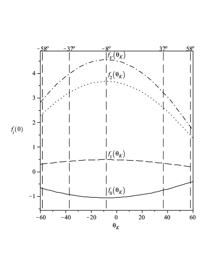
Figure 5: The dependence of the form factors on $\theta_{K_{1}}$ at $q^{2}=0$ for $D\to K_{1}(1270)\ell\nu$ decay.

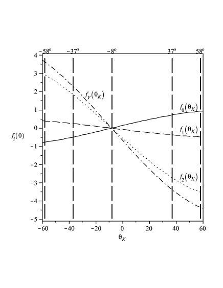
Figure 6: The dependence of the form factors on $\theta_{K_{1}}$ at $q^{2}=0$ for $D\to K_{1}(1400)\ell\nu$ decay.

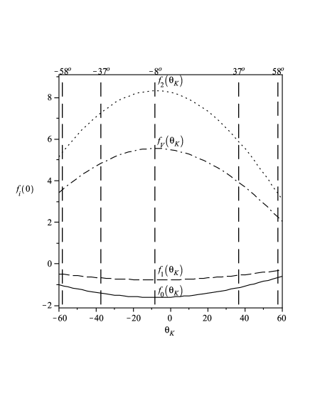
Figure 7: The dependence of the form factors on $\theta_{K_{1}}$ at $q^{2}=0$ for $D_{s}\to K_{1}(1270)\ell\nu$ decay.

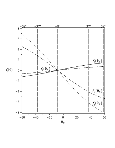
Figure 8: The dependence of the form factors on $\theta_{K_{1}}$ at $q^{2}=0$ for $D_{s}\to K_{1}(1400)\ell\nu$ decay.

The dependence of the $f_{i}^{D_{q}\to K_{1}}(0)$ on $\theta_{K_{1}}$ at $q^{2}=0$ is depicted in Figs. 5-8, in the interval $-58^{\circ}\leq\theta_{K_{1}}\leq 58^{\circ}$. In Figs. 6 and 8, as it is seen, all of the form factors contact at one point. Also each form factor in Figs. 5 and 7, has one extremum point. These extrema as well as the contact points have been specified in Figs. 5-8. It is interesting that in the $D_{q}\to K_{1}(1270)\ell\nu$ and $D_{q}\to K_{1}(1400)\ell\nu$ cases, the extrema and contact points of the form factors are nearly at $-8^{\circ}$. The sum rules for the form factors are truncated at about $q^{2}=0.15~{}GeV^{2}$ and $q^{2}=0.25~{}GeV^{2}$ for $q=u(d)$ and s cases of the $K_{1}(1270)$, respectively. These points for $K_{1}(1400)$ state are $q^{2}=0.22~{}GeV^{2}$ and $q^{2}=0.32~{}GeV^{2}$ for u(d) and s cases, respectively. To extend the results to the full physical region, i.e., $0\leq q^{2}\leq(m_{D_{q}}-m_{K_{1}})^{2}~{}GeV^{2}$, we look for a parametrization such that: 1) this parametrization coincides well with the sum rules predictions below the points at which the form factors are truncated and 2) the parametrization provides an extrapolation to $q^{2}>$ the truncated points, which is consistent with the expected analytical properties of the form factors and reproduces the lowest-lying resonance (pole). This resonance in the $D_{q}$ channel is $D^{*}(J^{P}=1^{-})$ state. Following references [26, 27], which describe this point in details, we choose the following theoretically more reliable fit parametrization:

$$f_{i}(q^{2})=\frac{a}{1-\frac{q^{2}}{m^{2}_{D^{*}}}}+\frac{b}{1-\frac{q^{2}}{m^{2}_{fit}}}.$$ (37)

The values of the parameters $a,~{}b$ and $m_{fit}$ are given in Tables 3-6 at different values of the mixing angle $\theta_{K_{1}}$. From this parametrization, we see that the $m_{D^{*}}$ pole exist outside the allowed physical region and related to that, one can calculate the hadronic parameters such as the coupling constant $g_{DD^{*}K_{1}}$ (see [28, 29]).

	$a$	$b$	$m_{fit}$		$a$	$b$	$m_{fit}$
$f_{V}^{D\to K_{1}(1270)}(q^{2})$	3.83	-0.64	1.25	$f_{V}^{D\to K_{1}(1400)}(q^{2})$	-5.94	2.57	1.25
$f_{0}^{D\to K_{1}(1270)}(q^{2})$	-2.05	1.31	1.36	$f_{0}^{D\to K_{1}(1400)}(q^{2})$	2.04	-1.32	1.36
$f_{1}^{D\to K_{1}(1270)}(q^{2})$	0.46	-0.12	1.27	$f_{1}^{D\to K_{1}(1400)}(q^{2})$	-0.59	0.21	1.27
$f_{2}^{D\to K_{1}(1270)}(q^{2})$	2.97	-0.41	1.29	$f_{2}^{D\to K_{1}(1400)}(q^{2})$	-3.14	0.44	1.29
$f_{V}^{D_{s}^{+}\to K_{1}^{0}(1270)}(q^{2})$	4.08	-0.18	1.28	$f_{V}^{D_{s}^{+}\to K_{1}^{0}(1400)}(q^{2})$	-7.87	3.78	1.28
$f_{0}^{D_{s}^{+}\to K_{1}^{0}(1270)}(q^{2})$	-3.56	2.41	1.51	$f_{0}^{D_{s}^{+}\to K_{1}^{0}(1400)}(q^{2})$	3.06	-1.94	1.51
$f_{1}^{D_{s}^{+}\to K_{1}^{0}(1270)}(q^{2})$	-0.70	0.16	1.31	$f_{1}^{D_{s}^{+}\to K_{1}^{0}(1400)}(q^{2})$	0.58	-0.01	1.31
$f_{2}^{D_{s}^{+}\to K_{1}^{0}(1270)}(q^{2})$	7.12	-1.23	1.35	$f_{2}^{D_{s}^{+}\to K_{1}^{0}(1400)}(q^{2})$	-5.32	-0.87	1.35

Table 3: Parameters appearing in the fit function for the form factors of the $D_{q}\to K_{1}(1270)\ell\nu$ and $D_{q}\to K_{1}(1400)\ell\nu$ decays at $M_{1}^{2}=8~{}GeV^{2}$, $M_{2}^{2}=6~{}GeV^{2}$ and $\theta_{K_{1}}=37^{\circ}$.

	$a$	$b$	$m_{fit}$		$a$	$b$	$m_{fit}$
$f_{V}^{D\to K_{1}(1270)}(q^{2})$	2.12	-0.30	1.27	$f_{V}^{D\to K_{1}(1400)}(q^{2})$	-7.44	3.10	1.27
$f_{0}^{D\to K_{1}(1270)}(q^{2})$	-1.52	1.10	1.37	$f_{0}^{D\to K_{1}(1400)}(q^{2})$	2.70	-1.78	1.37
$f_{1}^{D\to K_{1}(1270)}(q^{2})$	0.27	-0.08	1.29	$f_{1}^{D\to K_{1}(1400)}(q^{2})$	-0.75	0.26	1.29
$f_{2}^{D\to K_{1}(1270)}(q^{2})$	1.68	-0.22	1.31	$f_{2}^{D\to K_{1}(1400)}(q^{2})$	-4.00	0.51	1.31
$f_{V}^{D_{s}^{+}\to K_{1}^{0}(1270)}(q^{2})$	1.29	0.93	1.30	$f_{V}^{D_{s}^{+}\to K_{1}^{0}(1400)}(q^{2})$	-9.18	3.91	1.30
$f_{0}^{D_{s}^{+}\to K_{1}^{0}(1270)}(q^{2})$	-2.14	1.49	1.53	$f_{0}^{D_{s}^{+}\to K_{1}^{0}(1400)}(q^{2})$	4.03	-2.59	1.53
$f_{1}^{D_{s}^{+}\to K_{1}^{0}(1270)}(q^{2})$	-0.45	0.14	1.32	$f_{1}^{D_{s}^{+}\to K_{1}^{0}(1400)}(q^{2})$	0.79	-0.06	1.32
$f_{2}^{D_{s}^{+}\to K_{1}^{0}(1270)}(q^{2})$	4.78	-1.42	1.37	$f_{2}^{D_{s}^{+}\to K_{1}^{0}(1400)}(q^{2})$	-7.57	-0.40	1.37

Table 4: Parameters appearing in the fit function for the form factors of the $D_{q}\to K_{1}(1270)\ell\nu$ and $D_{q}\to K_{1}(1400)\ell\nu$ decays at $M_{1}^{2}=8~{}GeV^{2}$, $M_{2}^{2}=6~{}GeV^{2}$ and $\theta_{K_{1}}=58^{\circ}$.

	$a$	$b$	$m_{fit}$		$a$	$b$	$m_{fit}$
$f_{V}^{D\to K_{1}(1270)}(q^{2})$	5.48	-1.48	1.23	$f_{V}^{D\to K_{1}(1400)}(q^{2})$	2.81	-0.54	1.23
$f_{0}^{D\to K_{1}(1270)}(q^{2})$	-2.95	2.02	1.33	$f_{0}^{D\to K_{1}(1400)}(q^{2})$	-1.71	1.22	1.33
$f_{1}^{D\to K_{1}(1270)}(q^{2})$	0.61	-0.17	1.25	$f_{1}^{D\to K_{1}(1400)}(q^{2})$	0.35	-0.12	1.25
$f_{2}^{D\to K_{1}(1270)}(q^{2})$	3.90	-0.66	1.29	$f_{2}^{D\to K_{1}(1400)}(q^{2})$	2.10	-0.28	1.29
$f_{V}^{D_{s}^{+}\to K_{1}^{0}(1270)}(q^{2})$	7.23	-2.37	1.27	$f_{V}^{D_{s}^{+}\to K_{1}^{0}(1400)}(q^{2})$	2.10	0.66	1.27
$f_{0}^{D_{s}^{+}\to K_{1}^{0}(1270)}(q^{2})$	-4.27	2.83	1.48	$f_{0}^{D_{s}^{+}\to K_{1}^{0}(1400)}(q^{2})$	-2.43	1.67	1.48
$f_{1}^{D_{s}^{+}\to K_{1}^{0}(1270)}(q^{2})$	-0.80	0.14	1.30	$f_{1}^{D_{s}^{+}\to K_{1}^{0}(1400)}(q^{2})$	-0.54	0.15	1.30
$f_{2}^{D_{s}^{+}\to K_{1}^{0}(1270)}(q^{2})$	7.05	0.28	1.36	$f_{2}^{D_{s}^{+}\to K_{1}^{0}(1400)}(q^{2})$	5.62	-1.44	1.36

Table 5: Parameters appearing in the fit function for the form factors of the $D_{q}\to K_{1}(1270)\ell\nu$ and $D_{q}\to K_{1}(1400)\ell\nu$ decays at $M_{1}^{2}=8~{}GeV^{2}$, $M_{2}^{2}=6~{}GeV^{2}$ and $\theta_{K_{1}}=-37^{\circ}$.

	$a$	$b$	$m_{fit}$		$a$	$b$	$m_{fit}$
$f_{V}^{D\to K_{1}(1270)}(q^{2})$	3.86	-0.91	1.24	$f_{V}^{D\to K_{1}(1400)}(q^{2})$	4.88	-1.28	1.24
$f_{0}^{D\to K_{1}(1270)}(q^{2})$	-2.17	1.49	1.35	$f_{0}^{D\to K_{1}(1400)}(q^{2})$	-2.57	1.80	1.35
$f_{1}^{D\to K_{1}(1270)}(q^{2})$	0.44	-0.10	1.26	$f_{1}^{D\to K_{1}(1400)}(q^{2})$	0.56	-0.18	1.26
$f_{2}^{D\to K_{1}(1270)}(q^{2})$	2.97	-0.61	1.27	$f_{2}^{D\to K_{1}(1400)}(q^{2})$	3.38	-0.48	1.27
$f_{V}^{D_{s}^{+}\to K_{1}^{0}(1270)}(q^{2})$	5.73	-2.15	1.29	$f_{V}^{D_{s}^{+}\to K_{1}^{0}(1400)}(q^{2})$	4.88	-0.48	1.29
$f_{0}^{D_{s}^{+}\to K_{1}^{0}(1270)}(q^{2})$	-3.14	2.07	1.49	$f_{0}^{D_{s}^{+}\to K_{1}^{0}(1400)}(q^{2})$	-3.70	2.50	1.49
$f_{1}^{D_{s}^{+}\to K_{1}^{0}(1270)}(q^{2})$	-0.58	0.08	1.32	$f_{1}^{D_{s}^{+}\to K_{1}^{0}(1400)}(q^{2})$	-0.78	0.17	1.32
$f_{2}^{D_{s}^{+}\to K_{1}^{0}(1270)}(q^{2})$	4.69	0.71	1.35	$f_{2}^{D_{s}^{+}\to K_{1}^{0}(1400)}(q^{2})$	7.84	-1.20	1.35

Table 6: Parameters appearing in the fit function for the form factors of the $D_{q}\to K_{1}(1270)\ell\nu$ and $D_{q}\to K_{1}(1400)\ell\nu$ decays at $M_{1}^{2}=8~{}GeV^{2}$, $M_{2}^{2}=6~{}GeV^{2}$ and $\theta_{K_{1}}=-58^{\circ}$.

At the end of this section, we would like to discuss the numeric values of the differential decay rates as well as the branching ratios for the considered semileptonic and nonleptonic transitions.

semileptonic

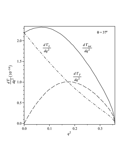
Figure 10: The dependence of the $d\Gamma_{tot}/dq^{2}$, $d\Gamma_{T}/dq^{2}$ and $d\Gamma_{L}/dq^{2}$ on $q^{2}$ at $\theta_{K_{1}}=37^{\circ}$ for $D^{+}\to K_{1}^{0}(1270)\ell\nu$.

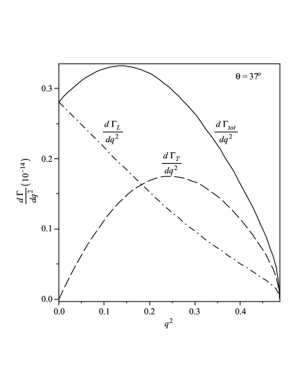
Figure 11: The dependence of the $d\Gamma_{tot}/dq^{2}$, $d\Gamma_{T}/dq^{2}$ and $d\Gamma_{L}/dq^{2}$ on $q^{2}$ at $\theta_{K_{1}}=37^{\circ}$ for $D^{+}_{s}\to K_{1}^{0}(1270)\ell\nu$.

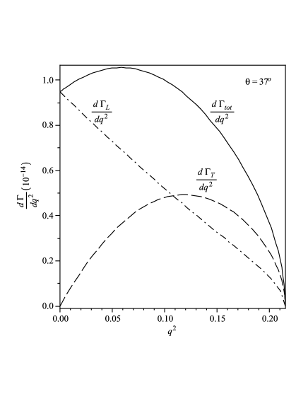
Figure 12: The dependence of the $d\Gamma_{tot}/dq^{2}$, $d\Gamma_{T}/dq^{2}$ and $d\Gamma_{L}/dq^{2}$ on $q^{2}$ at $\theta_{K_{1}}=37^{\circ}$ for $D^{0}\to K_{1}^{-}(1400)\ell\nu$.

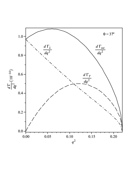
Figure 13: The dependence of the $d\Gamma_{tot}/dq^{2}$, $d\Gamma_{T}/dq^{2}$ and $d\Gamma_{L}/dq^{2}$ on $q^{2}$ at $\theta_{K_{1}}=37^{\circ}$ for $D^{+}\to K_{1}^{0}(1400)\ell\nu$.

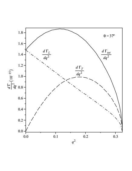
Figure 14: The dependence of the $d\Gamma_{tot}/dq^{2}$, $d\Gamma_{T}/dq^{2}$ and $d\Gamma_{L}/dq^{2}$ on $q^{2}$ at $\theta_{K_{1}}=37^{\circ}$ for $D^{+}_{s}\to K_{1}^{0}(1400)\ell\nu$.

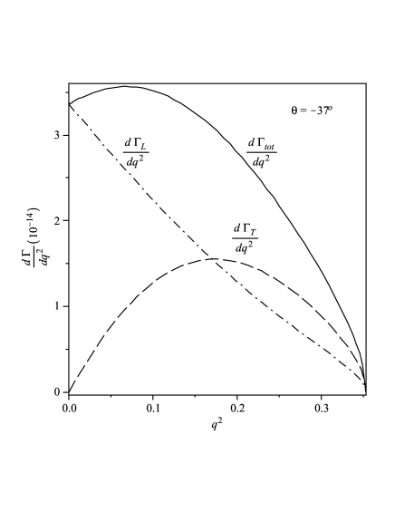
Figure 15: The dependence of the $d\Gamma_{tot}/dq^{2}$, $d\Gamma_{T}/dq^{2}$ and $d\Gamma_{L}/dq^{2}$ on $q^{2}$ at $\theta_{K_{1}}=-37^{\circ}$ for $D^{0}\to K_{1}^{-}(1270)\ell\nu$.

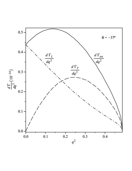
Figure 17: The dependence of the $d\Gamma_{tot}/dq^{2}$, $d\Gamma_{T}/dq^{2}$ and $d\Gamma_{L}/dq^{2}$ on $q^{2}$ at $\theta_{K_{1}}=-37^{\circ}$ for $D^{+}_{s}\to K_{1}^{0}(1270)\ell\nu$.

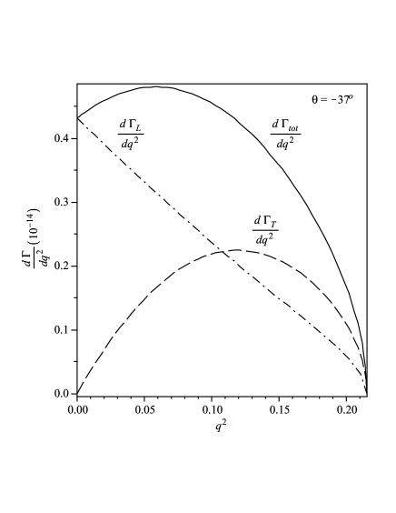
Figure 18: The dependence of the $d\Gamma_{tot}/dq^{2}$, $d\Gamma_{T}/dq^{2}$ and $d\Gamma_{L}/dq^{2}$ on $q^{2}$ at $\theta_{K_{1}}=-37^{\circ}$ for $D^{0}\to K_{1}^{-}(1400)\ell\nu$.

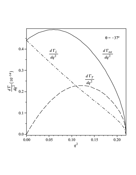
Figure 19: The dependence of the $d\Gamma_{tot}/dq^{2}$, $d\Gamma_{T}/dq^{2}$ and $d\Gamma_{L}/dq^{2}$ on $q^{2}$ at $\theta_{K_{1}}=-37^{\circ}$ for $D^{+}\to K_{1}^{0}(1400)\ell\nu$.

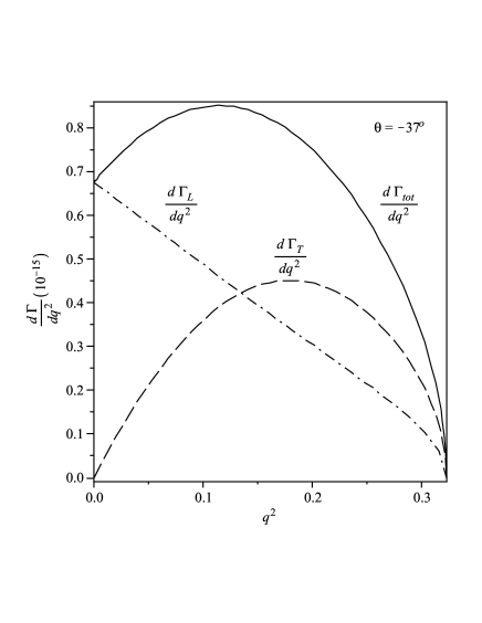
Figure 20: The dependence of the $d\Gamma_{tot}/dq^{2}$, $d\Gamma_{T}/dq^{2}$ and $d\Gamma_{L}/dq^{2}$ on $q^{2}$ at $\theta_{K_{1}}=-37^{\circ}$ for $D^{+}_{s}\to K_{1}^{0}(1400)\ell\nu$.

The dependence of the longitudinal and transverse components of the differential decay width for the semileptonic $D_{q}\to K_{1}\ell\nu$ decays is shown in Figs. 9-20 at $\theta_{K_{1}}=\pm 37^{\circ}$. In these figures, the total decay widths related to each decay are also depicted. To calculate the branching ratios of the semileptonic decays, we Integrate Eq. (30) over $q^{2}$ in the whole physical region and using the total mean life-time $\tau_{D^{0}}=0.41~{}ps$, $\tau_{D^{+}}=1.04~{}ps$ and $\tau_{D_{s}}=0.50~{}ps$ [23]. The values for the branching ratio of these decays are obtained as presented in Table 7.

$\theta_{K_{1}}^{\circ}$	37	58	-37	-58
$Br(D^{0}\to K_{1}^{-}(1270)\ell\nu)$	$[3.59\pm 0.29$	$1.03\pm 0.10$	$5.34\pm 0.21$	$2.84\pm 0.25]\times 10^{-3}$
$Br(D^{+}\to K_{1}^{0}(1270)\ell\nu)$	$[9.47\pm 0.45$	$2.70\pm 0.25$	$14.07\pm 1.22$	$7.57\pm 0.35]\times 10^{-3}$
$Br(D_{s}^{+}\to K_{1}^{0}(1270)\ell\nu)$	$[7.84\pm 0.41$	$2.09\pm 0.24$	$12.51\pm 1.16$	$6.91\pm 0.32]\times 10^{-4}$
$Br(D^{0}\to K_{1}^{-}(1400)\ell\nu)$	$[1.09\pm 0.10$	$1.78\pm 0.15$	$0.85\pm 0.02$	$1.20\pm 0.11]\times 10^{-3}$
$Br(D^{+}\to K_{1}^{0}(1400)\ell\nu)$	$[2.93\pm 0.25$	$4.75\pm 0.29$	$1.27\pm 0.10$	$3.20\pm 0.27]\times 10^{-3}$
$Br(D_{s}^{+}\to K_{1}^{0}(1400)\ell\nu)$	$[3.44\pm 0.29$	$5.88\pm 0.34$	$1.49\pm 0.13$	$3.96\pm 0.29]\times 10^{-4}$

Table 7: The values for the branching ratio of the semileptonic $D_{q}\to K_{1}(1270)\ell\nu$ and $D_{q}\to K_{1}(1400)\ell\nu$ decays at different values of the $\theta_{K_{1}}$.

The errors in this Table are estimated by the variation of the Borel parameters $M_{1}^{2}$ and $M_{2}^{2}$, the variation of the continuum thresholds $s_{0}$ and $s_{0}^{\prime}$ and uncertainties in the values of the other input parameters.

nonleptonic

For estimating the branching ratio of the nonleptonic $D\rightarrow K_{1}\pi$ decay, first the values of the form factors at $q^{2}=m_{\pi}^{2}$ are calculated as shown in Table 8.

$\theta_{K_{1}}^{\circ}$	37	58	-37	-58	$\theta_{K_{1}}^{\circ}$	37	58	-37	-58
$f_{V}^{D\to K_{1}(1270)}$	3.24	1.82	4.04	2.95	$f_{V}^{D\to K_{1}(1400)}$	-3.45	-4.42	2.30	3.65
$f_{0}^{D\to K_{1}(1270)}$	-0.73	-0.42	-0.91	-0.67	$f_{0}^{D\to K_{1}(1400)}$	0.70	0.92	-0.47	-0.75
$f_{1}^{D\to K_{1}(1270)}$	0.34	0.20	0.45	0.32	$f_{1}^{D\to K_{1}(1400)}$	-0.36	-0.49	0.25	0.41
$f_{2}^{D\to K_{1}(1270)}$	2.67	1.55	3.32	2.49	$f_{2}^{D\to K_{1}(1400)}$	-2.81	-3.65	1.87	3.03

Table 8: The values of the form factors of the $D\to K_{1}(1270)$ and $D\to K_{1}(1400)$ for $M_{1}^{2}=8~{}GeV^{2}$, $M_{2}^{2}=6~{}GeV^{2}$ at $q^{2}=m_{\pi}^{2}$ and different values of the mixing angle $\theta_{K_{1}}$.

Inserting these values in Eq. (36) and using $V_{ud}=0.97377\pm 0.00027$ [23], $m_{\pi}=0.139~{}GeV$ and $f_{\pi}=0.133~{}GeV$, we obtain the values for the branching ratio of these decays as presented in Table 9. In comparison, we also include the experimental values and upper limits in this Table. This Table shows that for the $D^{0}\to K_{1}^{-}(1270)\pi^{+}$, $D^{0}\to K_{1}^{-}(1400)\pi^{+}$ and $D^{+}\to K_{1}^{0}(1400)\pi^{+}$ cases, the different values of mixing angle $\theta_{K_{1}}$ give the values of branching ratios in good agreement with the experimental results but for $D^{+}\to K_{1}^{0}(1270)\pi^{+}$ decay, the values of the branching ratios at different values of $\theta_{K_{1}}$ are about one order of magnitude more than that of the experimental expectation.

$\theta_{K_{1}}^{\circ}$	37	58	-37	-58	Exp [23]
$Br(D^{0}\to K_{1}^{-}(1270)\pi^{+})\times 10^{-2}$	$1.45\pm 0.11$	$0.75\pm 0.06$	$2.26\pm 0.18$	$1.23\pm 0.11$	$1.15\pm 0.32$
$Br(D^{+}\to K_{1}^{0}(1270)\pi^{+})\times 10^{-2}$	$3.75\pm 0.29$	$1.23\pm 0.10$	$5.85\pm 0.37$	$3.18\pm 0.25$	$<0.7$
$Br(D^{0}\to K_{1}^{-}(1400)\pi^{+})\times 10^{-2}$	$0.60\pm 0.04$	$1.00\pm 0.12$	$0.26\pm 0.02$	$0.73\pm 0.04$	$<1.2$
$Br(D^{+}\to K_{1}^{0}(1400)\pi^{+})\times 10^{-2}$	$2.57\pm 0.21$	$3.63\pm 0.31$	$1.71\pm 0.13$	$2.78\pm 0.24$	$3.8\pm 1.3$

Table 9: The branching ratios of the nonleptonic $D\to K_{1}(1270)\pi$ and $D\to K_{1}(1400)\pi$ decays at different values of $\theta_{K_{1}}$.

In summary, we analyzed the semileptonic $D_{q}\to K_{1}\ell\nu$ transition with $q=u,d,s$ in the framework of the three–point QCD sum rules and the nonleptonic $D\to K_{1}\pi$ decay within the factorization approach. We calculated $D_{q}$ to $K_{1}(1270)$ and $K_{1}(1400)$ transition form factors by separating the mixture of the $K_{1}(1270)$ and $K_{1}(1400)$ states. Using the transition form factors of the $D\to K_{1}$, we analyzed the nonleptonic $D\to K_{1}\pi$ decay. We also evaluated the decay amplitude and decay width of these decays in terms of the transition form factors. The branching ratios of these decays were also calculated at different values of the mixing angle $\theta_{K_{1}}$. For the non leptonic case, a comparison of the results for the branching ratios with the existing experimental results was also made.

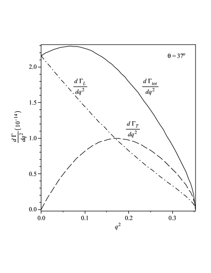
Figure 9: The dependence of the $d\Gamma_{tot}/dq^{2}$, $d\Gamma_{T}/dq^{2}$ and $d\Gamma_{L}/dq^{2}$ on $q^{2}$ at $\theta_{K_{1}}=37^{\circ}$ for $D^{0}\to K_{1}^{-}(1270)\ell\nu$.

Figure 16: The dependence of the $d\Gamma_{tot}/dq^{2}$, $d\Gamma_{T}/dq^{2}$ and $d\Gamma_{L}/dq^{2}$ on $q^{2}$ at $\theta_{K_{1}}=-37^{\circ}$ for $D^{+}\to K_{1}^{0}(1270)\ell\nu$.