Spontaneous magnetization in QCD and non-Fermi-liquid effects

Abstract

Magnetic properties of quark matter at finite temperature are discussed by evaluating the magnetic susceptibility. Combining the microscopic calculation of the self-energy for quarks as well as the screening effects for gluons with Fermi-liquid theory in a consistent way, we study the temperature dependence of the magnetic susceptibility. The longitudinal gluons have the static screening given by the Debye mass, and have a standard temperature dependence of $O(T^{2})$. An anomalous $T^{2}\ln T$ term arises in the magnetic susceptibility as a novel non-Fermi-liquid effect due to the anomalous self-energy for quarks given by the dynamic screening for transverse gluons. We then extract the critical (Curie) temperature and present the magnetic phase diagram on the density-temperature plane.

1 Introduction

Nowadays the phase diagram of QCD has been extensively studied theoretically by lattice calculations [1] and the effective models or experimentally by high-energy heavy-ion collisions (RHIC,LHC) [2] and observation of compact stars [3]. In particular, matter at high density but not high temperature should be interesting, since the Fermi surface is a good concept there and we can study interesting particle correlations such as superconducting pairing or instability of the Fermi surface in a clear way. It is also related with a quest of ”new form of matter” inside compact stars or during their thermal evolution [4].

We discuss here magnetic properties of QCD by the use of Fermi-liquid theory [5, 6, 7]. A possibility of spontaneous spin polarization has been suggested by one of the authors [8, 9], using the one-gluon-exchange (OGE) interaction. Higher-order calculations for the free energy have also supported this idea [9, 10]. If it is realized, it may give a microscopic origin of strong magnetic field observed in compact stars, especially magnetars [11]. The mechanism of spontaneous magnetization is very much similar to the one for the electron gas [12, 13, 14], where the leading-order contribution comes from the Fock exchange interaction. Electrons with the same spin can effectively avoid the repulsive Coulomb interaction due to the Pauli principle. On the other hand, the kinetic energy is increased as the number of each spin is different. Hence spontaneous polarization may occur at a peculiar density. Differences are color and flavor degrees of freedom for quark matter.

We apply the Landau Fermi-liquid theory (FLT) to elucidate the critical behavior of the magnetic phase transition at finite density and temperature. We evaluate the magnetization of quark matter by applying a small magnetic field $\bf B$. Then the magnetic susceptibility appears as a coefficient of the linear term in $B$. The divergence and sign change of the magnetic susceptibility signal the magnetic instability to the ferromagnetic phase, since its inverse measures the curvature of the free energy at the origin with respect to the magnetization. Thus quarks near the Fermi surface are responsible to the magnetic transition and the spin dependent quark-quark interaction and the density of states near the Fermi surface are the key ingredients within FLT .

In this theory, quarks are treated as quasi-particles and their energy $E$ is regarded as a functional of the distribution function. FLT is restricted to the low-lying excitations around the Fermi surface , where the lifetime of quasi-particles are long enough to be regarded as “particles” with properties resembling those of free particles. The single-particle energy is then given by the variation of $E$ with respect to the distribution function, incorporating the self-energy; the quasi-particle interactions are given by the variation of the single-particle energy with respect to the distribution function and they are specified by the set of a few parameters, called the Landau-Migdal parameters. It is well-known that there appear infrared (IR) singularities in the Landau-Migdal parameters in gauge theories (QED/QCD) since the gauge interaction is infinite range. To improve the IR behavior we must take into account the correlation effects for the quasi-particle interaction: we must sum up an infinite series of the most divergent diagrams as the self-energy term of the gauge field. Thus we take into account the screening effects for the gauge field. For example, the Coulomb interaction becomes “finite” range and there is left no singularity in the condensed-matter physics [6]. The summation of the infinite series or the inclusion of the screening effects is also required by the argument of the hard-dense-loop (HDL) resummation [18]. Consider the particle-hole polarization diagram as a leading-order contribution to the self-energy of the gauge field. Since the IR singularities appear for quasi-particles with the collinear momenta, the soft gluon should give a dominant contribution. Then the particle-hole polarization function $\Pi(q)\sim O(g^{2}\mu^{2})$ should be the same order of magnitude with the energy-momentum squared of gluons $\sim(g\mu)^{2}$. Hence we must sum up the infinite series, $1/q^{2}\left(1+\Pi/q^{2}+...\right)$, to get the meaningful results. For the longitudinal mode we can see the static screening by the Debye mass and the IR behavior is surely improved. On the other hand, there is no static screening for the transverse mode but only the dynamic screening due to the Landau damping[18]. Thus the IR singularities still remain in the Landau-Migdal parameters derived through the exchange of the gauge boson of the transverse mode.

In a recent paper we studied the screening effects for gluons to evaluate the magnetic susceptibility of quark matter at $T=0$ within FLT [19, 20]. We have seen that the transverse gluons still give logarithmic singularities to the Landau-Migdal parameters, but they cancel each other in the magnetic susceptibility to give a finite result. Finally the static screening for the longitudinal gluons gives the $g^{4}{\rm ln}(1/g^{2})$ term in the magnetic susceptibility [13, 21]. A similar term is also obtained as a correlation effect in electron gas and the ferromagnetic region is diminished. However, we also find that this term has an interesting behavior in QCD, depending on the number of flavors. Consequently the screening effect does not necessarily work against the magnetic instability, which is a different aspect from electron gas.

In this paper, we extend our previous analysis to the finite-temperature case and figure out the non-Fermi-liquid aspect of the magnetic susceptibility. Since thermal gluons should give higher-order terms in $T$, we only consider the interacting quark system within FLT. We take into account the effect of the self-energy of quasi-particles by using the explicit expression given by the perturbation method. We shall see that the longitudinal gluons give little temperature dependence due to the static screening, while the transverse gluons exhibit an anomalous temperature dependence for the magnetic susceptibility through the dynamic screening. Shanker has shown that the application of the renormalization group (RG) automatically leads to FLT as a fixed-point, where all the quasi-particle interactions are marginal [22], except the attractive superconducting (BCS) channel. This argument, however, may be applied to the case of the short-range interaction. Recent RG arguments have revealed that the quasi-particle interaction through the exchange of the transverse gauge bosons is relevant and induces the non-Fermi-liquid effects in gauge theories (QED/QCD) [16, 24, 30, 31]. Furthermore, it should be important to note that quasi-particle interaction is infrared free, so that the effective coupling becomes very weak when the excitation energy of the quasi-particles from the Fermi surface approaches to null [16]. The effective coupling constant is given by the product of the gauge coupling constant $g^{2}$ and the Fermi velocity $v_{F}$, $C_{\rm eff}=g^{2}v_{F}/4\pi$. Since $v_{F}$ goes to zero on the Fermi surface, the perturbation method should be meaningful even if the gauge coupling is not weak.

The quasi-particle energy $\epsilon_{\bf k}$ should be given by the root of the transcendental equation, $\epsilon_{\bf k}=E_{\bf k}+{\rm Re}\Sigma_{+}(\epsilon_{\bf k},{\bf k})$ with $E_{\bf k}=(|{\bf k}|^{2}+m^{2})^{1/2}$, and the one-loop result of the self-energy $\Sigma_{+}(\epsilon_{\bf k},{\bf k})$ by way of the microscopic many-body technique exhibits an anomalous behavior as $\epsilon_{\bf k}\rightarrow\mu$, ${\rm Re}\Sigma_{+}(\epsilon_{\bf k})\sim\gamma(\epsilon_{\bf k}-\mu){\rm ln}(\Lambda/|\epsilon_{\bf k}-\mu|)$ with $\gamma=g^{2}/9\pi^{2}$, due to the dynamic screening [24, 25]. The further analysis of the self-energy by way of the Schwinger-Dyson equation or the renormalization group have shown that the anomalous term in the one-loop result is reliable even if $\gamma\ln(\Lambda/|\epsilon_{\bf k}-\mu|)\sim 1$: actually there is no difference between the one-loop result and the solution of the Schwinger-Dyson equation [16]. Consequently, the renormalization factor $z_{+}(k)=(1-\partial{\rm Re}\Sigma_{+}(\omega)/\partial\omega)^{-1}|_{\omega=\epsilon_{\bf k}}$ vanishes at $k=k_{F}$, which means that the distribution function has no discontinuity at $\epsilon_{k_{F}}=\mu$ even at $T=0$, or there is no Fermi surface [6, 26, 27]. However, the distribution function of the quasi-particles is still the step function at $T=0$. Actually we have seen that the transverse mode causes no effect for the instability of the Fermi surface due to its sharpness [19].

At $T\neq 0$, the Fermi surface is diffused over the width of $O(T)$ , so that the transverse gluons should give rise to an anomalous logarithmic dependence for physical quantities through the dynamic screening, as we shall see in the following. For instance, the anomaly in the specific heat has been repeatedly discussed in the literatures [24, 28, 29, 30, 31, 32, 33]; the transverse gauge field gives a $T\ln T$ term as a leading-order contribution. Analogous non-Fermi-liquid behavior can be also seen in the context of color superconductivity at high densities [34, 35, 36, 37]. We shall see that there appears a $T^{2}\ln T$ term in the magnetic susceptibility as another non-Fermi-liquid effect [38]. This temperature dependence is different from that of the specific heat, while one may naively expect the same one by considering the density of states on the Fermi surface: the leading-order contribution is $\ln T$, but it is canceled by another $\ln T$ term coming from the spin-dependent Landau-Migdal parameter to leave the next-to-leading-order term of $T^{2}\ln T$ in the magnetic susceptibility.

To extract the temperature dependence correctly we must consider the temperature dependence of the chemical potential as well. We derive it within FLT and show that the result is the same as that given by a microscopic calculation [32]. Properly taking into account the temperature dependence of the chemical potential, which also includes the $T^{2}\ln T$ term, we finally present the magnetic susceptibility at finite temperature.

If the magnetic susceptibility diverges at some density and some temperature, it signals the magnetic instability of quark matter to the ferromagnetic phase. Thus we can extract the critical densities and temperatures to draw a critical curve on the density-temperature plane. Using our results, we shall demonstrate the magnetic phase diagram, which might be useful in considering some phenomenological implications of magnetism of quark matter. We get several tens MeV as the maximum critical (Curie) temperature. This value is similar to that expected during supernova explosion, so that it would be interesting to consider the thermal evolution of magnetars in the initial cooling stage.

In this work we sometimes need the explicit result of a microscopic calculation rather than general framework of FLT. In each step of the calculation we try to figure out the difference and similarity, compared with the usual discussion of FLT.

In §2 a framework is presented within Fermi-liquid theory to study the magnetic properties of quark matter. In §3 non-Fermi-liquid effects are extracted in the magnetic susceptibility at finite temperature. Some specific temperature dependence of chemical potential is also discussed. In §4 a magnetic phase diagram is presented on the density-temperature plane, where we can also see an importance of the non-Fermi-liquid effect. Some relations between the microscopic calculation and the FLT are summarized in Appendix B.

2 Fermi-liquid theory for quark matter

Within the Landau Fermi-liquid theory (FLT) we assume a one-to-one correspondence between the states of the free Fermi gas and those of the interacting system. Quarks are treated as quasi-particles carrying the same quantum numbers of the free particles, and the quasi-particle distribution function is simply given by the Fermi-Dirac one,

$$n({\bf k},\zeta)=\left[1+\exp(\beta(\epsilon_{{\bf k},\zeta}-\mu))\right]^{-1}$$ (1)

with the quasi-particle energy $\epsilon_{{\bf k},\zeta}$ specified by the momentum ${\bf k}$ and a spin quantum number $\zeta=\pm 1$.

Since “spin” is not a good quantum number in relativistic theories, we specify the polarization of each quark by introducing the spin vector $a^{\mu}$, which is a covariant generalization of the spin direction $\bm{\zeta}$ (we take it along $z-$axis) in the non-relativistic case. Actually spin vector $a^{\mu}$ is a space-like four vector with the constraints, $a^{\mu}k_{\mu}=0$ and $a^{2}=-1$, and it is reduced to the three vector $\bm{\zeta}$ in the rest frame. It is not uniquely given, but there are many choices for the explicit form of spin vector. We must choose the most relevant one for the description of ferromagnetic phase[8]. Here we assume the standard form [39, 40],

$${\bf a}=\bm{\zeta}+\frac{{\bf k}(\bm{\zeta}\cdot{\bf k})}{m(E_{k}+m)},~{}~{}~{}a^{0}=\frac{{\bf k}\cdot\bm{\zeta}}{m},$$ (2)

with $E_{k}=({\bf k}^{2}+m^{2})^{1/2}$.

We can define an eigenstate $u^{(\zeta)}$ of the operator, $W\cdot a$, where $W^{\mu}$ is the Pauli-Lubanski vector, $W_{\mu}=-1/4\epsilon_{\mu\nu\rho\sigma}k^{\nu}\sigma^{\rho\sigma}$:

$$-\frac{W\cdot a}{m}u^{(\zeta)}=\frac{\zeta}{2}u^{(\zeta)},$$ (3)

with $\zeta=\pm 1$. Accordingly we can define polarization density matrix $\rho(k,\zeta)$,

$$\rho(k,\zeta)=\frac{1}{2m}(k/+m)P(a),$$ (4)

by the projection operator, $P(a)=1/2\cdot(1+\gamma_{5}a/)$.

2.1 Quasi-particle interaction

Since the color-singlet magnetization is not directly related to the color degree of freedom, we, hereafter, only consider the color-symmetric interaction among quasi-particles that can be written as the sum of two parts, the spin symmetric ($f^{s}_{{\bf k},{\bf q}}$) and anti-symmetric ($f^{a}_{{\bf k},{\bf q}}$) terms;

$$f_{{\bf k}\zeta,{\bf q}\zeta^{\prime}}=f^{s}_{{\bf k},{\bf q}}+\zeta\zeta^{\prime}f^{a}_{{\bf k},{\bf q}}.$$ (5)

Since quark matter is color singlet as a whole, the Fock exchange interaction gives a leading contribution [41]. We, hereafter, take a perturbation technique and consider the one-gluon-exchange interaction (OGE) with relatively large coupling constant. One may wonder the perturbation method should break in that case. However, the real expansion parameter is not the gauge coupling constant in the present case; RG argument has shown that the quasi-particle interaction is infrared free and the effective coupling becomes very weak for the low-lying excitations around the Fermi surface[16]. The effective coupling constant is then given by the product of the gauge coupling constant $g^{2}$ and the Fermi velocity $v_{F}$, $C_{\rm eff}=g^{2}v_{F}/4\pi$, and $v_{F}$ becomes vanished on the Fermi surface. Hence the perturbation method is meaningful even if the gauge coupling is not weak.

For a pair with color index $(a,b)$, the Fock exchange interaction gives a factor $(\lambda_{\alpha})_{ab}(\lambda_{\alpha})_{ba}=1/2-1/(2N_{c})\delta_{ab}$, which is always positive for any pair. Hence the situation is very similar to electron gas in QED. Since we are interested in the electromagnetic properties of quark matter, only the color symmetric interaction is relevant, which is written as

$$f_{{\bf k}\zeta,{\bf q}\zeta^{\prime}}=\frac{1}{N_{c}^{2}}\sum_{a,b}f_{{\bf k}\zeta a,{\bf q}\zeta^{\prime}b}=\frac{m}{E_{k}}\frac{m}{E_{q}}M_{{\bf k}\zeta,{\bf q}\zeta^{\prime}},$$ (6)

with the invariant matrix element,

$$M_{{\bf k}\zeta,{\bf q}\zeta^{\prime}}=-g^{2}\frac{1}{N_{c}^{2}}{\rm tr}\left(\lambda_{\alpha}/2\lambda_{\alpha}/2\right)M^{\mu\nu}(k,\zeta;q,\zeta^{\prime})D_{\mu\nu}(k-q),$$ (7)

where $M^{\mu\nu}(k,\zeta;q,\zeta^{\prime})={\rm tr}\left[\gamma^{\mu}\rho(k,\zeta)\gamma^{\nu}\rho(q,\zeta^{\prime})\right]$. The matrix elements are easily evaluated with the definition of the density matrix $\rho(k,\zeta)$ (Eq. (4)) and summarized in Appendix A. Since the OGE interaction is a long-range force and we consider the small energy-momentum transfer between quasi-particles, we must treat the gluon propagator by taking into account HDL resummation [18]. Thus we take into account the screening effect,

$$D_{\mu\nu}(k-q)=P^{t}_{\mu\nu}D_{t}(p)+P^{l}_{\mu\nu}D_{l}(p)-\xi\frac{p_{\mu}p_{\nu}}{p^{4}}$$ (8)

with $p=k-q$, where $D_{t(l)}(p)=(p^{2}-\Pi_{t(l)})^{-1}$, and the last term represents the gauge dependence with a parameter $\xi$. $P^{t(l)}_{\mu\nu}$ is the projection operator onto the transverse (longitudinal) mode,

$$P^{t}_{\mu\nu} = (1-g_{\mu 0})(1-g_{\nu 0})\left(-g_{\mu\nu}-\frac{p_{\mu}p_{\nu}}{|{\bf p}|^{2}}\right)$$

$$P^{l}_{\mu\nu} = -g_{\mu\nu}+\frac{p_{\mu}p_{\nu}}{p^{2}}-P^{t}_{\mu\nu}.$$ (9)

The self-energies for the transverse and longitudinal gluons are given as

$$\Pi_{l}(p_{0},{\bf p}) = \sum_{f=u,d,s}\left(m_{D,f}^{2}+i\frac{\pi m_{D,f}^{2}}{2u_{F,f}}\frac{p_{0}}{|{\bf p}|}\right)$$

$$\Pi_{t}(p_{0},{\bf p}) = -i\sum_{f=u,d,s}\frac{\pi u_{F,f}m_{D,f}^{2}}{4}\frac{p_{0}}{|{\bf p}|},$$ (10)

in the limit $p_{0}/|{\bf p}|\rightarrow 0$, with $u_{F,f}\equiv k_{F,f}/E_{F,f}$ and the Debye mass for each flavor, $m_{D,f}^{2}\equiv g^{2}\mu_{f}k_{F,f}/2\pi^{2}$ [18] . Thus the longitudinal gluons are statically screened to have the Debye mass, while the transverse gluons are dynamically screened by the Landau damping, in the limit $p_{0}/|{\bf p}|\rightarrow 0$. Accordingly, the screening effect for the transverse gluons is ineffective at $T=0$, where soft gluons ($p_{0}/|{\bf p}|\rightarrow 0$) contribute. At finite temperature, gluons with $p_{0}\sim O(T)$ can contribute due to the diffuseness of the Fermi surface and the transverse gluons are effectively screened.

2.2 Magnetic susceptibility

We consider the linear response of the normal(unpolarized) quark matter by applying a small magnetic field $\bf B$. The magnetic susceptibility is defined as

$$\chi_{M}=\sum_{f=u,d,s}\chi_{M}^{f}=\sum_{f=u,d,s}\left.\frac{\partial\langle M\rangle_{f}}{\partial B}\right|_{B=0}$$ (11)

with the magnetization $\langle M\rangle_{f}$ for each flavor, where we take ${\bf B}//\hat{\bf z}$. We consider here the spin susceptibility, so that the magnetization is given by $\langle M\rangle_{f}=V^{-1}\langle\int d^{3}x{\bar{q}}_{f}\Sigma_{z}q_{f}\rangle$ with $\mu_{q}^{f}$ being the Dirac magnetic moment. Hereafter, we shall concentrate on one flavor and omit the flavor indices because the magnetic susceptibility is given by the sum of the contribution from each flavors. Magnetic susceptibility is then written in terms of the quasi-particle interaction [5, 20],

$$\chi_{M}=\left(\frac{\bar{g}_{D}\mu_{q}}{2}\right)^{2}\frac{N(T)}{1+N(T)\bar{f}^{a}}$$ (12)

where $\bar{g}_{D}=\int_{|{\bf k}|=k_{F}}d\Omega_{\bf k}/4\pi g_{D}({\bf k})$ is the gyromagnetic ratio ,

$$g_{D}({\bf k})\zeta=2{\rm tr}\left[\Sigma_{z}\rho(k,\zeta)\right]=2\left(a_{z}-\frac{k_{z}}{E_{k}}a_{0}\right),$$ (13)

and can be explicitly written as

$$g_{D}({\bf k})=2\left[1-\frac{k_{z}^{2}}{E_{k}(E_{k}+m)}\right],$$ (14)

using the spin vector (Eq. (2)).

$N(T)$ is the effective density of states on the Fermi surface, and defined by

$$N(T)=-\int_{-\infty}^{\infty}d\omega\frac{\partial n(\omega)}{\partial\omega}\nu(\omega),$$ (15)

where $n(\omega)$ is the Fermi-Dirac distribution function and $\nu(\omega)$ is the density of states of the quasi-particles at energy $\omega$,

$$\nu(\omega)\equiv-\frac{2N_{c}}{\pi}\int\frac{d^{3}k}{(2\pi)^{3}}{\rm Im}\left[{\cal S}_{+}^{R}(\omega,{\bf k})\right],$$ (16)

in terms of the retarded Green function of the quasi-particles, ${\cal S}_{+}^{R}(\omega,{\bf k})=(\omega-\epsilon_{\bf k}-i\eta)^{-1}$. The quasi-particle energy $\epsilon_{\bf k}$ is given by the kinetic energy $E_{\bf k}=\sqrt{{\bf k}^{2}+m^{2}}$ and the self-energy $\Sigma_{+}(\epsilon_{\bf k},{\bf k})$,

$$\epsilon_{\bf k}=E_{\bf k}+\Sigma_{+}(\epsilon_{\bf k},{\bf k}).$$ (17)

Since $n(\omega)\rightarrow\theta(\mu-\omega)$ as $T\rightarrow 0$, $N(T)$ is reduced to the effective density of states at the Fermi surface of the quasi-particles at $T=0$, $N(0)=N_{c}k_{F}^{2}/\pi^{2}v_{F}$ with the Fermi velocity, $v_{F}=(\partial\epsilon_{\bf k}/\partial k)_{k=k_{F}}$. Note that $-\partial n(\omega)/\partial\omega$ is sharply peaked at $\omega=\mu$ for $T/\mu\ll 1$ which we are concerned with, and we can see that only the quasi-particles with the energy $\epsilon_{\bf k}\simeq\mu$ still gives a dominant contribution .

$\bar{f}^{a}$ is a Landau-Migdal parameter defined by

$${\bar{f}^{a}}\equiv-2N_{c}\int\frac{d^{3}k}{(2\pi)^{3}}\frac{\partial n(\epsilon_{\bf k})}{\partial\epsilon_{\bf k}}{\bar{f}}^{a}_{k,k_{s}}/N(T)$$ (18)

after angle-averaged over the Fermi surface,

$${\bar{f}^{a}}_{k,k_{s}}\equiv\int\frac{d\Omega_{\bf k}}{4\pi}\int\frac{d\Omega_{\bf q}}{4\pi}\left.f^{a}_{{\bf k},{\bf q}}\right|_{|{\bf q}|=k_{s}},$$ (19)

where $k_{s}$ is defined by $\epsilon_{k_{s}}=\mu$ and coincides with the usual Fermi momentum $k_{F}$ at $T=0$.

3 Non-Fermi-liquid behavior at finite temperature

We consider the magnetic susceptibility at low temperature. In the usual FLT it should have little temperature dependence, while we shall see that the anomalous $T^{2}\ln T$ term appears due to the dynamic screening effect; the anomalous term is a leading-order contribution at low temperature. To show such term we carefully analyze the self-energy $\Sigma_{+}(\epsilon_{\bf k})$, the derivative of which logarithmically diverges as $\epsilon_{\bf k}\rightarrow\mu$.

3.1 Average of the density of states near $\epsilon_{\bf k}=\mu$

In this subsection, we study the average of the density of state given by Eq. (15). As we shall see, we can not use the usual low-temperature expansion because of the singularity of the quasi-particle energy at the Fermi surface. Therefore, more careful treatment is needed.

First, we substitute Eq. (16) into Eq. (15) and change the variable of integration in Eq. (15) from $k$ to $\epsilon_{\bf k}(=\omega)$;

$$N(T)=\frac{N_{c}}{\pi^{2}}\int_{\epsilon_{0}}^{\infty}d\omega\frac{dk}{d\omega}k^{2}\frac{\beta e^{\beta\left(\omega-\mu\right)}}{\left(e^{\beta\left(\omega-\mu\right)}+1\right)^{2}},$$ (20)

with $\epsilon_{0}\equiv\epsilon_{|{\bf k}|=0}$. The quasi-particle energy $\omega$ satisfies the relation,

$$\omega=E_{k(\omega)}+{\rm Re}\Sigma_{+}(\omega,k(\omega)),$$ (21)

where we discard the imaginary part within the quasi-particle approximation.

The one-loop self-energy is almost independent of the momentum, and can be written as [24, 25]

$${\rm Re}\Sigma_{+}(\omega,k)\sim{\rm Re}\Sigma_{+}(\mu,k_{F}) -\frac{C_{f}g^{2}u_{F}}{12\pi^{2}}(\omega-\mu)\ln\frac{\Lambda}{|\omega-\mu|}$$

$$+\Delta^{\rm reg}(\omega-\mu)$$ (22)

and

$${\rm Im}\Sigma_{+}(\omega,k)\sim\frac{C_{f}g^{2}}{24\pi}|\omega-\mu|+O\left((\omega-\mu)^{2}\right)$$ (23)

around $\omega\sim\mu$ with $C_{f}=(N_{c}^{2}-1)/(2N_{c})$ and $u_{F}=k_{F}/E_{k_{F}}$. $\Lambda$ is a cut-off factor and should be an order of the Debye mass. (In this paper, we take $\Lambda=M_{D}=\sqrt{\sum_{f}m_{D,f}^{2}}$.) Note that the anomalous term in Eq. (22) appears from the dynamic screening of the transverse gluons, and the contribution by the longitudinal gluons is summarized in the regular function $\Delta^{\rm reg}(\omega-\mu)$ of $O(g^{2})$. Within the approximation given by Eqs. (22) and (23), the self-energy is independent of spatial momentum $k$ and thus we omit the argument $k$ hereafter. The renormalization factor $z_{+}(k)$ is then given by the equation, $z_{+}(k)=(1-\partial{\rm Re}\Sigma_{+}(\omega)/\partial\omega|_{\omega=\epsilon_{\bf k}})^{-1}$, and we have

$$z_{+}(k)^{-1}\sim-\frac{C_{f}g^{2}u_{F}}{12\pi^{2}}\ln|\epsilon_{\bf k}-\mu|.$$ (24)

It exhibits a logarithmic divergence as $\epsilon_{\bf k}\rightarrow\mu$, which causes non-Fermi-liquid behavior [16].

Differentiating Eq. (21) with respect to $k$, we find

$$\frac{dk(\omega)}{d\omega}\simeq\left(1-\frac{\partial{\rm Re}\Sigma_{+}(\omega)}{\partial\omega}\right)\frac{E_{k(\omega)}}{k(\omega)}.$$ (25)

Here, we have used $\partial{\rm Re}\Sigma_{+}/\partial k\simeq 0$ for the self-energy Eq. (22).

Eventually, $N(T)$ is written as,

$$N(T)\simeq\frac{N_{c}}{\pi^{2}}\int_{\epsilon_{0}}^{\infty}d\omega\left(1-\frac{\partial{\rm Re}\Sigma_{+}(\omega)}{\partial\omega}\right)k(\omega)E_{k(\omega)}\frac{\beta e^{\beta\left(\omega-\mu\right)}}{\left(e^{\beta\left(\omega-\mu\right)}+1\right)^{2}}.$$ (26)

As is discussed in Appendix B, we can separate the contribution by the longitudinal gluons $N_{l}(T)$ from $N(T)$. Since the longitudinal gluon exchange is short-ranged by the Debye screening mass, it becomes almost temperature independent,

$$N_{l}(T)=\frac{N_{c}k_{F}E_{F}}{3\pi^{2}}f_{l;1}^{s},$$ (27)

with the Landau-Migdal parameter $f_{l;1}^{s}$,

$$f_{l;1}^{s}=-\frac{3N_{c}^{-1}C_{f}g^{2}}{8E_{F}^{2}k_{F}^{2}}\left[\kappa k_{F}^{2}+2E_{F}^{2}\right]\left[(1+\kappa)I_{0}(\kappa)-1\right],$$ (28)

where $\kappa=\sum_{f}m_{D,f}^{2}/2k_{F}^{2}$ and

$$I_{0}(\kappa) = \frac{1}{2}\int_{-1}^{1}\frac{du}{1-u+\kappa}\simeq\frac{1}{2}{\rm ln}\left(\frac{2}{\kappa}\right)\simeq{\rm ln}(g^{-2}).$$ (29)

To evaluate the transverse contribution, $N_{t}(T)=N(T)-N_{l}(T)$, we only use the transverse part in Eq. (22): substituting Eq. (22) into Eq. (26), we obtain the leading-order contribution ,

$$N_{t}(T)=\frac{N_{c}k_{s}\mu}{\pi^{2}}\Big{[}1+\frac{\pi^{2}}{6}\frac{(2k_{F}^{2}-m^{2})}{k_{F}^{4}}T^{2}\\ +\frac{C_{f}g^{2}u_{F}}{24}\frac{(2k_{F}^{2}-m^{2})}{k_{F}^{4}}T^{2}\ln\left(\frac{\Lambda}{T}\right)+\frac{C_{f}g^{2}u_{F}}{12\pi^{2}}\ln\left(\frac{\Lambda}{T}\right)\Big{]}+O(g^{2}T^{2}),$$ (30)

after some manipulation (Appendix C). $N_{t}(T)$ has a term proportional to $\ln T$, which gives a singularity at $T=0$. This singularity corresponds to the logarithmic divergence of the Landau-Migdal parameter $f_{1}^{s}$ at $T=0$ (Appendix B). Inverting this for $T\neq 0$, we find

$$N^{-1}(T)=\frac{\pi^{2}}{N_{c}k_{s}\mu}\Big{[}1-\frac{\pi^{2}}{6}\frac{(2k_{F}^{2}-m^{2})}{k_{F}^{4}}T^{2}\\ -\frac{C_{f}g^{2}u_{F}}{72}\frac{(2k_{F}^{2}-m^{2})}{k_{F}^{4}}T^{2}\ln\left(\frac{\Lambda}{T}\right)-\frac{C_{f}g^{2}u_{F}}{12\pi^{2}}\ln\left(\frac{\Lambda}{T}\right)\Big{]}-N_{l}(T)+O(g^{2}T^{2}).$$ (31)

Note that this formula is meaningful only at nonzero temperature; a renormalization group argument tells that theory is infrared free in this case and the perturbation analysis of the low energy behavior is reliable [16]. We have kept the next-to-leading term ($T^{2}\ln T$ term) as well as the leading-order term ($\ln T$ term), since we shall see that the $\ln T$ term is canceled out by another term appearing in the spin-dependent Landau-Migdal parameter $\bar{f}^{a}$ in the magnetic susceptibility.

3.2 Cancellation of the singular terms at $T=0$

At finite temperature, the magnetic susceptibility is given by

$$\chi_{M}=\left(\frac{\bar{g}_{D}\mu_{q}}{2}\right)^{2}\left[N^{-1}(T)+\bar{f}_{l}^{a}+\bar{f}_{t}^{a}\right]^{-1}$$ (32)

where $\bar{f}_{l}^{a}$ and $\bar{f}_{t}^{a}$ denote the longitudinal and transverse parts of $\bar{f}^{a}$ respectively. $\bar{f}^{a}_{t}$ has the logarithmic singularity, which comes from the OGE interaction between quarks with collinear momenta. The longitudinal component $\bar{f}_{l}^{a}$ has no IR singularity because of the static screening and is almost temperature independent as $f_{l;1}^{s}$ in Eq. (27).

The leading-order contribution at finite temperature comes from the transverse component $\bar{f}_{t}^{a}$; it has a logarithmic singularity at $T=0$ due to the dynamic screening effect. In this section, we shall see that the logarithmic divergences of $N^{-1}(T)$ and $\bar{f}_{t}^{a}$ at $T=0$ cancel out each other to give a finite contribution to the magnetic susceptibility. $\bar{f}_{t}^{a}$ is given by

$$\bar{f}_{t}^{a}=-2N_{c}N^{-1}(T)\int\frac{d^{3}k}{(2\pi)^{3}}\frac{\partial n(\epsilon_{\bf k})}{\partial\epsilon_{{\bf k}}}\bar{f}^{a}_{{t};k,k_{s}}$$ (33)

with

$$\bar{f}^{a}_{t:k,k_{s}} =-\left.\int\frac{d\Omega_{\bf k}}{4\pi}\int\frac{d\Omega_{\bf q}}{4\pi}\frac{m^{2}}{E_{s}E_{\bf k}}C_{f}N_{c}^{-1}g^{2}M^{iia}D_{t}(k-q)\right|_{|{\bf q}|=k_{s}}$$ (34)

where $M^{iia}$ is the spin-dependent component of $M^{ii}$ in Eq.(7) (see Appendix A) and we have defined $E_{s}$ by $E_{s}=E_{|{\bf q}|=k_{s}}$. It is the dynamic screening part in the propagator $D_{t}$ that gives the $\ln T$ dependence to $\bar{f}^{a}_{t}$. Therefore, we can put $|{\bf k}|=k_{s}$ in the other parts of the integrand in Eq. (34). Then,

$$M^{iia}=\frac{k_{s}^{2}}{4m^{2}}\left[1+\cos\theta_{\widehat{{\bf k}{\bf q}}}+\cos\theta_{\bf k}\cos\theta_{\bf q}-\cos\theta_{\bf k}^{2}-\cos\theta_{\bf q}^{2}\right].$$ (35)

The real part of the transverse propagator is

$${\rm Re}D_{t}(k-q)\Big{|}_{|{\bf q}|=k_{s}} =\frac{(k-q)^{2}}{\left\{(k-q)^{2}\right\}^{2}+\left(\frac{1}{4}\sum_{f}\pi u_{F,f}m_{D,f}^{2}\right)^{2}\frac{(E_{\bf k}-E_{s})^{2}}{({\bf k}-{\bf q})^{2}}}\Bigg{|}_{|{\bf q}|=k_{s}}$$

$$\simeq-\frac{1}{2k_{s}^{2}}\frac{(1-\cos\theta_{\widehat{{\bf k}{\bf q}}})^{2}}{(1-\cos\theta_{\widehat{{\bf k}{\bf q}}})^{3}+c^{3}(E_{\bf k}-E_{s})^{2}}$$ (36)

with $c^{3}\equiv\frac{1}{8k_{s}^{6}}\left(\sum_{f}\frac{\pi m_{D,f}^{2}u_{F,f}}{4}\right)^{2}$, while the imaginary part is given by

$${\rm Im}D_{t}(k-q)\Big{|}_{|{\bf q}|=k_{s}}=\frac{2\sqrt{2}k_{s}^{3}c^{3/2}\frac{(E_{\bf k}-E_{s})}{|{\bf k}-{\bf q}|}}{\left\{(k-q)^{2}\right\}^{2}+8k_{s}^{6}c^{3}\frac{(k_{0}-q_{0})^{2}}{({\bf k}-{\bf q})^{2}}}\Bigg{|}_{|{\bf q}|=k_{s}}.$$ (37)

It is easily shown that the imaginary part gives $\bar{f}^{a}$ only higher-order terms with respect to temperature and thus we neglect it here. Performing the angular integrals in Eq. (34),

$$\bar{f}^{a}_{t;k,k_{s}}=\frac{C_{f}N_{c}^{-1}g^{2}}{48E_{s}^{2}}\Big{[}-10+2\ln\Big{|}\frac{c^{3}(E_{\bf k}-E_{s})^{2}+8}{c^{3}(E_{\bf k}-E_{s})^{2}}\Big{|}\\ +\frac{5c(E_{\bf k}-E_{s})^{2/3}}{6}\ln\Big{|}\frac{(c(E_{\bf k}-E_{s})^{2/3}+2)^{3}}{c^{3}(E_{\bf k}-E_{s})^{2}+8}\Big{|}\\ +\frac{5c(E_{\bf k}-E_{s})^{2/3}}{6}\tan^{-1}\left(\frac{4-c(E_{\bf k}-E_{s})^{2/3}}{\sqrt{3}c(E_{\bf k}-E_{s})^{2/3}}\right)\\ +\frac{5\pi}{6\sqrt{3}}c(E_{\bf k}-E_{s})^{2/3}\Big{]}$$ (38)

For small $|E_{\bf k}-E_{s}|\sim O(T)$, it reads

$$\bar{f}_{t;k,k_{s}}^{a} \sim-\frac{C_{f}N_{c}^{-1}g^{2}}{8E_{s}^{2}}\ln\left[\frac{c(E_{\bf k}-E_{s})^{2/3}}{2}\right]$$ (39)

The integral in Eq. (33) can be performed as in the case of $N(T)$, Eq. (20). Changing the variable of integration from $k$ to $\omega$, we find

$$\bar{f}_{t}^{a}\simeq\frac{N_{c}}{\pi^{2}T}N^{-1}(T)\int_{\epsilon_{0}}^{\infty}d\omega k(\omega)E_{k(\omega)}\left(1-\frac{\partial{\rm Re}\Sigma_{+}(\omega)}{\partial\omega}\right)\bar{f}^{a}_{t;k(\omega),k_{s}}\frac{e^{\beta(\omega-\mu)}}{\left(e^{\beta(\omega-\mu)}+1\right)^{2}}.$$ (40)

Note that $\partial{\rm Re}\Sigma_{+}(\omega)/\partial\omega$ in the integrand does not contribute as long as we calculate to $O(g^{2})$ as $\bar{f}^{a}_{k(\omega),t}$ itself is $O(g^{2})$. Integrating Eq. (40) as in Appendix C and using Eq. (31), we find a leading-order contribution at $T\neq 0$,

$$\bar{f}_{t}^{a} \sim N^{-1}(T)\frac{C_{f}g^{2}}{12\pi^{2}k_{s}E_{s}}\left[1+\frac{\pi^{2}}{6}\frac{(2k_{s}^{2}-m^{2})}{k_{s}^{4}}T^{2}\right]\ln T^{-1}+O(g^{2}T^{2})$$

$$\sim\frac{C_{f}g^{2}}{12N_{c}E_{s}\mu}\ln T^{-1}.$$ (41)

Compare Eq. (41) with Eq. (31). Since $E_{s}=E_{F}+O(T^{2})$ and $k_{s}=k_{F}+O(T^{2})$ as we shall see, the $\ln T$ terms cancel each other in the magnetic susceptibility (32). In Fig.1, we plot $\pi^{2}/(N_{c}k_{s}\mu)-N^{-1}_{t}(T)$, $\bar{f}^{a}_{t}$, and $N^{-1}_{t}(T)+\bar{f}^{a}_{t}$ at $k_{F}=1.0$ fm^-1 near $T=0$. As is shown, both $N_{t}^{-1}(T)$ and $\bar{f}^{a}_{t}$ are singular at $T=0$, but a cancellation occurs so that the sum of the two becomes finite even at $T=0$. Thus we can take the limit $T\rightarrow 0$ in the magnetic susceptibility.

It is also worthwhile to note that $N_{t}(T)+\bar{f}^{a}_{t}$ seems to be almost temperature-independent in the unit of $\pi^{2}/(N_{c}k_{s}\mu)=1$ in Fig. 1. However, the chemical potential has the implicit temperature dependence. We shall discuss this $T$-dependence in the following.

\psfrag{N}{$\frac{\pi^{2}}{(N_{c}k_{s}\mu)}-N^{-1}_{t}(T)$}\psfrag{f}{{$\bar{f}^{a}_{t}$}}\psfrag{S}{$N^{-1}_{t}(T)+\bar{f}^{a}_{t}$}\includegraphics[width=260.17464pt]{Figure1.eps}

Figure 1: Cancellation of the logarithmic terms. $\pi^{2}/(N_{c}k_{s}\mu)-N^{-1}_{t}(T)$, $\bar{f}^{a}_{t}$, and $N^{-1}_{t}(T)+\bar{f}^{a}_{t}$ are plotted for $\Lambda=M_{D}$ and $k_{F}=1.0$ fm^-1 in the unit of $\pi^{2}/(N_{c}k_{s}\mu)=1$. $\bar{f}^{a}_{t}$ and $N^{-1}_{t}(T)$ are singular at $T=0$, but they cancel each other and the magnetic susceptibility remains finite even at $T=0$.

3.3 Magnetic susceptibility at T=0

Before presenting the full expression of the temperature dependence, it would be interesting to see how to recover the result at $T=0$ [19, 20]. We have seen that the logarithmic terms in $N_{t}(T)^{-1}$ and $\bar{f}^{a}_{t}$ cancel each other to leave the regular terms in the magnetic susceptibility at $T=0$. One can easily check that there arises no more singular terms from the longitudinal contribution $\bar{f}^{a}_{l}$ at $T=0$, since the longitudinal gluons are screened by the Debye mass $M_{D}$. The Landau-Migdal parameter $\bar{f}^{a}_{l}$ is given by

$$\bar{f}_{l}^{a}=-2N_{c}N^{-1}(T)\int\frac{d^{3}k}{(2\pi)^{3}}\frac{\partial n(\epsilon_{\bf k})}{\partial\epsilon_{{\bf k}}}\bar{f}^{a}_{l;k,k_{s}}$$ (42)

with

$$\bar{f}^{a}_{l;k,k_{s}} =-\left.\int\frac{d\Omega_{\bf k}}{4\pi}\int\frac{d\Omega_{\bf q}}{4\pi}\frac{m^{2}}{E_{s}E_{\bf k}}C_{f}N_{c}^{-1}g^{2}M^{00a}D_{l}(k-q)\right|_{|{\bf q}|=k_{s}}$$ (43)

in the same way as $\bar{f}^{a}_{t}$, where $M^{00a}$ is the spin-dependent component of $M^{00}$ in Eq.(7) (see Appendix A). Now the gluon propagator $D_{l}(k-q)$ has no infrared singularity, so that

$$\bar{f}_{l}^{a} \simeq\bar{f}^{a}_{l;k_{s},k_{s}}$$

$$=-\left.\int\frac{d\Omega_{\bf k}}{4\pi}\int\frac{d\Omega_{\bf q}}{4\pi}\frac{m^{2}}{E_{F}^{2}}C_{f}N_{c}^{-1}g^{2}M^{00a}D_{l}(k-q)\right|_{|{\bf k}|=|{\bf q}|=k_{F}}+O(g^{2}T^{2}).$$ (44)

Consequently $\bar{f}^{a}_{l}$ has little temperature dependence, and can be written as

$$\bar{f}^{a}_{l} =-\frac{C_{f}g^{2}N_{c}^{-1}}{8E_{F}^{2}k_{F}^{2}}\left[2E_{F}^{2}I_{0}(\kappa)+\frac{2}{3}\kappa(E_{F}-m)^{2}I_{0}(\kappa)\right.$$

$$+\left.\kappa\left\{k_{F}^{2}I_{0}(\kappa)+\frac{2}{3}\left((1+\kappa)I_{0}(\kappa)-1\right)(E_{F}-m)^{2}\right\}-k_{F}^{2}-\frac{2}{3}(E_{F}-m)^{2}\right]$$ (45)

with $\kappa=\sum_{f}m^{2}_{D,f}/2k_{F}^{2}$ at $T=0$ [19, 20]. Thus there is no singularity at $T=0$ in the magnetic susceptibility (32).

The magnetic susceptibility at $T=0$ is already given in ref. [19, 20],

$$\hskip 10.00002pt\left(\chi_{M}(T=0)/\chi_{\rm Pauli}\right)^{-1}$$

$$=\frac{N_{c}k_{F}\mu_{0}}{\pi^{2}}\left[N^{-1}(0)+\bar{f}^{a}_{l}+\bar{f}^{a}_{t}\right]$$

$$=1-\frac{C_{f}g^{2}\mu_{0}}{12\pi^{2}E_{F}^{2}k_{F}}\left[m(2E_{F}+m)-\frac{1}{2}\left(E_{F}^{2}+4E_{F}m-2m^{2}\right)\kappa\ln\frac{2}{\kappa}\right],$$ (46)

where $\chi_{\rm Pauli}$ is the Pauli paramagnetism, $\chi_{\rm Pauli}\equiv{\bar{g}}_{D}^{2}\mu_{q}^{2}N_{c}k_{F}\mu/4\pi^{2}$, and $\mu_{0}=E_{F}+O(g^{2})$ is the chemical potential at $T=0$. Using Eqs. (31), (41), (45) for the magnetic susceptibility (32) and comparing it with Eq. (46) at $T=0$, we find that they are different from each other by the temperature-independent term $C_{f}g^{2}k_{F}/24\pi^{2}E_{F}$, which is attributed to the contribution by the transverse gluons.

Note that the screening effect for the longitudinal gluons gives rise to the contribution of $g^{4}\ln(1/g^{2})$ [13, 21]. Obviously this expression (46) is reduced to the simple OGE case without screening in the limit $\kappa\rightarrow 0$; one can see that the interaction among massless quarks gives a null contribution for the magnetic transition.

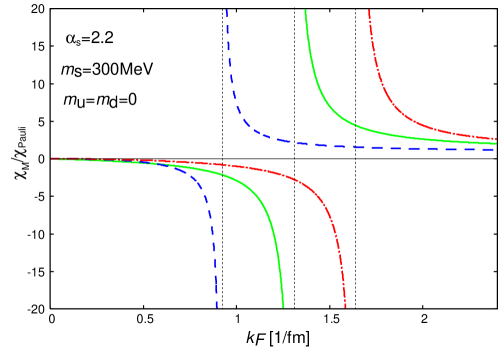
Figure 2: Magnetic susceptibility at $T=0$. The solid curve shows the result using simple OGE, while the dashed and dash-dotted ones show the screening effects with $N_{f}=1$(only s quarks) and with $N_{f}=3$(u, d, and s quarks) respectively.

In Fig. 2, we plot the magnetic susceptibility at $T=0$[19, 20]. We take the QCD coupling constant as $\alpha_{s}\equiv g^{2}/4\pi=2.2$ and the strange quark mass $m_{s}=300$MeV, inferred from the MIT bag model[42]. We consider here the MIT bag model as an effective model in our energy scale, which succeeds in reproducing the low-lying hadron spectra. The coupling constant looks rather large, but this value is required for the color magnetic interaction to explain the mass splitting of hadrons with different spins; e.g. for nucleon and $\Delta$ isobar. We think this feature is relevant in our study, because the coupling constant is closely related to the strength of the spin-spin interaction between quarks in this model. Moreover, the quark density in the MIT bag model is moderate, $\sim 0.25$fm^-3, which is the similar one we are here interested in. Note that the perturbation method should be still meaningful even for this rather large coupling, since the renormalization-group analysis has shown that the relevant expansion parameter is not the gauge coupling constant $g^{2}$ but the product of $g^{2}$ with the Fermi velocity $v_{F}$, which always goes to zero as one approaches to the Fermi surface [16].

One can see that the magnetic susceptibility for the simple OGE without screening diverges around $k_{F}=1.3$ fm ^-1. This is consistent with the previous result for the energy calculation. [19, 20]. One may expect that the screening effect weakens the Fock exchange interaction so that the critical density get lower once we take into account the screening effect. However, this is not necessarily the case in QCD. The screening effect behaves in different ways depending on the number of flavors. Compare the results for the $N_{f}=3$ with the one for $N_{f}=1$. In the case of $N_{f}=1,\kappa\leq 2$ the screening effect works against the magnetic phase transition as in QED. However, for $N_{f}=3$, $\kappa>2$ so that the critical density is increased. Consequently the screening effect does not necessarily work against the magnetic instability, which is a different aspect from electron gas [20].

3.4 Temperature dependence of the chemical potential

The chemical potential $\mu$ in Eq. (31) implicitly includes the temperature dependence. To extract the proper temperature dependence in $\chi_{M}$ we must carefully take into account the temperature dependence of $\mu$ ; here we use the thermodynamic relation $\mu=-(\partial F/\partial n)|_{T}$ with the free energy $F=E-Ts$.

In the following we only consider the temperature variation $\delta T$, so that the contribution of the longitudinal gluons can be well discarded due to the Debye screening. Accordingly it is sufficient to take into account the contribution from the transverse gluons in Eq. (22). We shall see that $\mu$ includes $T^{2}\ln T$ term due to the dynamic screening effect for the transverse gluons, besides the usual $T^{2}$ term.

Using the fact that the temperature variation of the free energy equals $-s\delta T$, we calculate the quasi-particle entropy per unit volume $s$,

$$s=-N_{c}\sum_{\zeta}\int\frac{d^{3}k}{(2\pi)^{3}}\left[n({\bf k},\zeta)\ln n({\bf k},\zeta)+(1-n({\bf k},\zeta))\ln(1-n({\bf k},\zeta))\right]$$ (47)

for each flavor, and then integrate it with respect to temperature to get $F$. The temperature variation of $s$ is given as

$$\delta s=-\frac{1}{T}N_{c}\sum_{\zeta}\int\frac{d^{3}k}{(2\pi)^{3}}(\epsilon_{{\bf k},\zeta}-\mu)\delta n({\bf k},\zeta)$$ (48)

through the variation of the distribution function,

$$\delta n({\bf k},\zeta)=\frac{\partial n({\bf k},\zeta)}{\partial\epsilon_{{\bf k},\zeta}}\left[-\frac{\epsilon_{{\bf k},\zeta}-\mu}{T}\delta T+\delta\epsilon_{{\bf k},\zeta}-\delta\mu\right].$$ (49)

Since the term involving $\delta\epsilon_{{\bf k},\zeta}-\delta\mu$ gives at least $T^{3}\ln T$ in the entropy at low temperature [5], we shall see that the leading-order contribution is given by the term with the explicit temperature variation $\delta T$,

$$\delta s=-N_{c}\sum_{\zeta}\int\frac{d^{3}k}{(2\pi)^{3}}\frac{\partial n({\bf k},\zeta)}{\partial\epsilon_{{\bf k},\zeta}}(\epsilon_{{\bf k},\zeta}-\mu)^{2}\frac{\delta T}{T}.$$ (50)

Using Eq. (25), $\delta s$ is recast into the following form,

$$\delta s=\frac{1}{T^{3}}\frac{N_{c}}{\pi^{2}}\int d\omega k(\omega)E_{k(\omega)}\left(1-\frac{\partial{\rm Re}\Sigma_{+}(\omega)}{\partial\omega}\right)\frac{e^{\beta(\omega-\mu)}}{(e^{\beta(\omega-\mu)}+1)^{2}}(\omega-\mu)^{2}\delta T.$$ (51)

Changing the variable $\omega$ by $y$ s.t. $\omega-\mu=yT$ and using Eq. (22), we have

$$\delta s=\frac{N_{c}k_{F}E_{F}}{3}\left(1-\frac{C_{f}g^{2}u_{F}}{12\pi^{2}}\ln\left(\frac{T}{\Lambda}\right)+O(g^{2})\right)\delta T.$$ (52)

as in Appendix C. Thus the entropy is

$$s=\frac{N_{c}k_{F}E_{F}T}{3}\left(1-\frac{C_{f}g^{2}u_{F}}{12\pi^{2}}\ln\left(\frac{T}{\Lambda}\right)\right)+O(g^{2}T).$$ (53)

Note that this result is the same as the one given in ref.[32], and the non-Fermi-liquid behavior of the specific heat $c_{V}=T(\partial s/\partial T)_{V}=s+O(g^{2}T)$ is also reproduced. The free energy $F$ is then given by the integral of $s$ with respect to temperature,

$$F=E_{0}+\frac{N_{c}E_{F}k_{F}}{6}T^{2}+\frac{N_{c}C_{f}g^{2}k_{F}^{2}}{72\pi^{2}}T^{2}\ln\left(\frac{\Lambda}{T}\right)+O(g^{2}T^{2}),$$ (54)

where $E_{0}$ is the ground state energy at $T=0$. Through the thermodynamic relation $\mu=-(\partial F/\partial n)$ we finally obtain

$$\mu(T)=\mu_{0}-\frac{\pi^{2}}{6}\frac{2k_{F}^{2}+m^{2}}{k_{F}^{2}E_{F}}T^{2}\left(1+\frac{C_{f}g^{2}u_{F}}{12\pi^{2}}\ln\left(\frac{\Lambda}{T}\right)\right)+O(g^{2}T^{2}).$$ (55)

Note that this relation is also given by considering the total number density at finite temperature [32].

3.5 Temperature dependence of the magnetic susceptibility

One can easily find that temperature-dependent terms of $E_{s}$ is the same as those of $\mu(T)$ within the order we are interested in, noticing that $E_{s}=\mu-{\rm Re}\Sigma_{+}(\mu)$ and ${\rm Re}\Sigma_{+}(\mu)={\rm Re}\Sigma_{+}(\mu_{0})+O(g^{2}T^{2})$. Using $k_{s}=\sqrt{E_{s}^{2}-m^{2}}$, we find the temperature dependence of $k_{s}$,

$$k_{s}=k_{F}-\frac{\pi^{2}}{6}\frac{2k_{F}^{2}+m^{2}}{k_{F}^{3}}T^{2}\left(1+\frac{C_{f}g^{2}u_{F}}{12\pi^{2}}\ln\left(\frac{\Lambda}{T}\right)\right)+O(g^{2}T^{2}).$$ (56)

Now we can rewrite Eqs. (31) and (41) in terms of $k_{F}$ and $E_{F}$;

$$N^{-1}(T) =\frac{\pi^{2}}{N_{c}k_{F}\mu_{0}}\Big{[}1+\frac{\pi^{2}}{6k_{F}^{4}}\left(2E_{F}^{2}-m^{2}+\frac{m^{4}}{E_{F}^{2}}\right)T^{2}$$

$$-\frac{C_{f}g^{2}u_{F}}{72}\frac{2k_{F}^{2}-m^{2}}{k_{F}^{4}}T^{2}\ln\left(\frac{\Lambda}{T}\right)-\frac{C_{f}g^{2}u_{F}}{12\pi^{2}}\ln\left(\frac{\Lambda}{T}\right)\Big{]}-N_{l}(T)+O(g^{2}T^{2}).$$ (57)

and

$$\bar{f}_{\rm t}^{a}=\frac{C_{f}g^{2}}{12N_{c}E_{F}\mu_{0}}\left[1+\frac{\pi^{2}}{3k_{F}^{2}E_{F}^{2}}\left(2k_{F}^{2}+m^{2}\right)T^{2}\right]\ln T^{-1}+O(g^{2}T^{2}).$$ (58)

Taking into account this temperature dependence of the chemical potential and using Eqs. (57) and (58), we find the temperature dependence of $\delta\chi_{M}^{-1}$,

$$\delta\chi_{M}^{-1} =\chi_{\rm Pauli}^{-1}\Big{[}\frac{\pi^{2}}{6k_{F}^{4}}\left(2E_{F}^{2}-m^{2}+\frac{m^{4}}{E_{F}^{2}}\right)T^{2}$$

$$\hskip 50.00008pt+\frac{C_{f}g^{2}u_{F}}{72k_{F}^{4}E_{F}^{2}}\left(2k_{F}^{4}+k_{F}^{2}m^{2}+m^{4}\right)T^{2}\ln\left(\frac{\Lambda}{T}\right)\Big{]}+O(g^{2}T^{2}).$$ (59)

Finally we obtain the magnetic susceptibility at finite temperature by adding $\delta\chi^{-1}_{M}$ to Eq. (46),

$$\left(\chi_{M}/\chi_{\rm Pauli}\right)^{-1}=1-\frac{C_{f}g^{2}}{12\pi^{2}E_{F}k_{F}}\Big{[}m(2E_{F}+m)-\frac{1}{2}(E_{F}^{2}+4E_{F}m-2m^{2})\kappa\ln\frac{2}{\kappa}\Big{]}$$

$$+\frac{\pi^{2}}{6k_{F}^{4}}\left(2E_{F}^{2}-m^{2}+\frac{m^{4}}{E_{F}^{2}}\right)T^{2}+\frac{C_{f}g^{2}u_{F}}{72}\frac{(2k_{F}^{4}+k_{F}^{2}m^{2}+m^{4})}{k_{F}^{4}E_{F}^{2}}T^{2}\ln\left(\frac{\Lambda}{T}\right)$$

$$+O(g^{2}T^{2}).$$ (60)

There appears $T^{2}\ln T$ dependence in the susceptibility at finite temperature besides the usual $T^{2}$ dependence [20]. This corresponds to the $T\ln T$ term in the specific heat [24, 28, 29, 30, 31, 32, 33] and is a novel non-Fermi-liquid effect in the magnetic susceptibility. At low temperature, $\ln(\Lambda/T)>0$ so that the $T^{2}\ln T$ term gives positive contribution to $\chi_{M}^{-1}$. Therefore, both $T$-dependent terms in Eq. (60) work against the magnetic instability.

In Fig.3, we show the temperature dependence of the magnetic susceptibility at $k_{F}=1.0$ fm^-1 using Eqs.(59) and (60). The thin solid, dash-dotted, heavy solid, and dashed curves indicate $\delta\chi_{M}(T)/\chi_{\rm Pauli}$, $\chi_{M}(T=0)/\chi_{\rm Pauli}$, $\chi_{M}(T)/\chi_{\rm Pauli}$ and $(k_{F}\mu_{0})/(k_{s}\mu)$ for $\Lambda=M_{D}$ respectively. The temperature at which the heavy solid curve cross the zero corresponds to the critical(Curie) temperature. Temperature dependence of the magnetic susceptibility, i.e. $\delta\chi_{M}$ originates from the transverse gluons. $(k_{F}\mu_{0})/(k_{s}\mu)$ is rewritten as

$$\left(\frac{\bar{g}_{D}\mu_{q}}{2}\right)^{-2}\frac{\pi^{2}}{Nk_{s}\mu}\Big{/}\chi^{-1}_{\rm Pauli}$$ (61)

and corresponds to the first term in Eq.(31). Once we take into account the temperature dependence of the chemical potential, this term depends on temperature and adds temperature dependence other than the explicit temperature dependence to the magnetic susceptibility. We also plot the magnetic susceptibility with the temperature dependence of the chemical potential disregarded. If we ignore the temperature dependence of the chemical potential, the magnetic susceptibility hardly depend on temperature. The temperature dependence of the magnetic susceptibility almost comes from that of the chemical potential.

\psfrag{A}{\small$\delta\chi^{-1}_{M}(T)/\chi^{-1}_{\rm Pauli}$}\psfrag{B}{\small$\chi^{-1}_{M}(0)/\chi^{-1}_{\rm Pauli}$}\psfrag{D}{\small$\chi^{-1}_{M}(T)/\chi^{-1}_{\rm Pauli}$}\psfrag{E}{\small$(k_{F}\mu_{0})/(k_{s}\mu)$}\includegraphics[width=260.17464pt]{Figure3.eps}

Figure 3: Temperature dependence of the magnetic susceptibility at $k_{F}=1.0$ fm^-1. $\delta\chi^{-1}_{M}(T)/\chi^{-1}_{\rm Pauli}$, $\chi^{-1}_{M}(T=0)/\chi^{-1}_{\rm Pauli}$, $\chi^{-1}_{M}(T)/\chi^{-1}_{\rm Pauli}$, and $(k_{F}\mu_{0})/(k_{s}\mu)$ are plotted for $\Lambda=M_{D}$. The dotted curve is the magnetic susceptibility in which the temperature dependence of the chemical potential is neglected. The parameters are the same as those used in Fig. 1. $\chi^{-1}_{M}(T)$ changes its sign at $T=T_{c}$, which gives a critical (Curie) temperature.

4 Magnetic phase diagram of QCD on the density-temperature plane

In this section, we show some numerical results for the magnetic susceptibility at finite temperature. We consider a symmetric quark matter with three flavors in equal populations, massless $u,d$ quarks and massive $s$ quarks. We use the same values for $m$ and $\alpha_{s}$ as in Fig. 2.

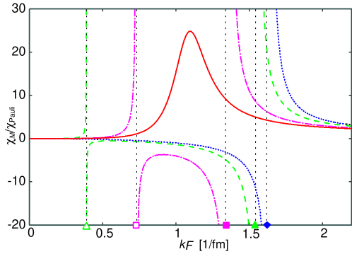
(a)

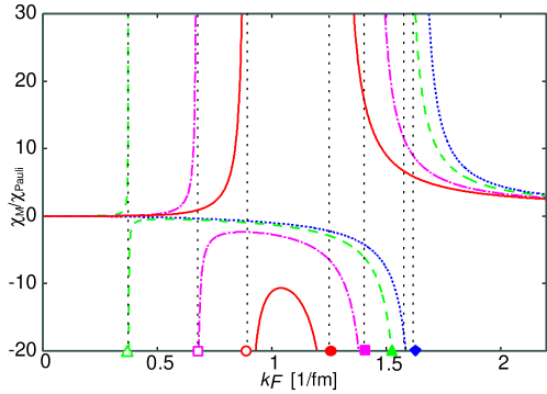
(b)

Figure 4: Magnetic susceptibility at finite temperature. The upper panel shows the result for the full expression, Eq.(60), while the lower one shows the result without the $T^{2}\ln T$ term in Eq.(60). The dotted, dashed, dash-dotted, and solid curves show the results at $T$=0, 30, 50, and 60 MeV respectively. The diamonds indicate the critical density, $k_{F}^{c}$ at $T=0$ and the open (filled) triangles, squares, and circles indicate $k_{F1}^{c}(k_{F2}^{c})$ for $T=$30, 50, and 60MeV respectively.

In Fig.4(a), we plot the magnetic susceptibility given by Eq. (60). At $T$=0, the magnetic susceptibility is positive at higher densities and the quark matter is in the paramagnetic phase there. At the critical density where the magnetic susceptibility diverges ($k_{F}^{c}\sim 1.6$fm^-1), there occurs a magnetic phase transition from the paramagnetic phase to the ferromagnetic phase and the quark matter remains ferromagnetic below $k_{F}^{c}$.

At $T=$30 MeV, there appear two critical densities at which the magnetic susceptibility diverges. We denote these densities $k_{F1}^{c}$ and $k_{F2}^{c}$ ($k_{F1}^{c}<k_{F2}^{c}$). In this case, $k_{F1}^{c}\simeq 0.4$fm^-1 and $k_{F2}^{c}\simeq 1.5$ fm^-1. At densities below $k_{F1}^{c}$ and above $k_{F2}^{c}$, the magnetic susceptibility is positive, which corresponds to the paramagnetic phase, on the other hand, at densities between two critical densities, it becomes negative corresponding to the ferromagnetic phase.

At $T=$50 MeV, there are still two critical densities ($k_{F1}^{c}\simeq 0.7$fm^-1 and $k_{F2}^{c}\simeq 1.3$fm^-1), but the range between these two densities becomes narrower than at $T=$30 MeV.

At $T=$60 MeV, there is no longer divergence in the magnetic susceptibility and the quark matter is paramagnetic at any density.

To figure out the non-Fermi-liquid effect, in Fig.4(b), we depict the magnetic susceptibility without the $T^{2}\ln T$ term in Eq.(60) for comparison: only $T^{2}$- dependence on temperature is taken into account. At $T=0$, there is no difference from the curve shown in Fig.4(a) and there is little difference between Fig.4(a) and (b) even at $T=$30 and 50 MeV. However, at $T=$60MeV, there is a region where the spontaneous magnetization is still realized in Fig.4(b), whereas the quark matter is paramagnetic at any density in Fig. 4(a). From these considerations, the non-Fermi-liquid effect lowers the Curie temperature to some extent and affects the magnetic property of quark matter in contrast with that of the anomalous specific heat ($\propto T\ln T$) in a non-relativistic electron gas [28, 29, 30, 31].

We show a magnetic phase diagram of QCD on the density-temperature plane in Fig.5. The four curves corresponds to the critical curves given by Eq.(60) under four different assumptions: below the curves the quark matter is in the ferromagnetic phase, while it is in the paramagnetic phase above the critical curves. The magnetic transition occurs on the critical curves.

For the solid curve, we have used the full expression Eq.(60), on the other hand, for the dashed, dash-dotted, and dotted curves, we have ignored the dynamic screening(i.e. the $T^{2}\ln T$ term), static screening(i.e. the $\kappa\ln\kappa$ term), and both of the two screenings in Eq. (60) respectively.

Compare the result with the full expression (60) with the one without the non-Fermi-liquid effect i.e. $T^{2}\ln T$ dependence. In the case without the $T^{2}\ln T$ term, the ferromagnetic phase can be sustained till over $T=60$ MeV, while it can be at most $T=60$MeV including $T^{2}\ln T$ dependence. It turns out that the dynamic screening works against the magnetic instability and can reduce the ferromagnetic region in the phase diagram up to a point, but this effect is not so large.

The dash-dotted curve is the result without the static screening or $\kappa\ln\kappa$ term in Eq.(60). The static screening effect works in favor of the magnetic instability to enlarge the ferromagnetic region. As discussed in  [20], it depends on the number of flavors whether the static screening works for the ferromagnetism or not, which is peculiar to QCD.

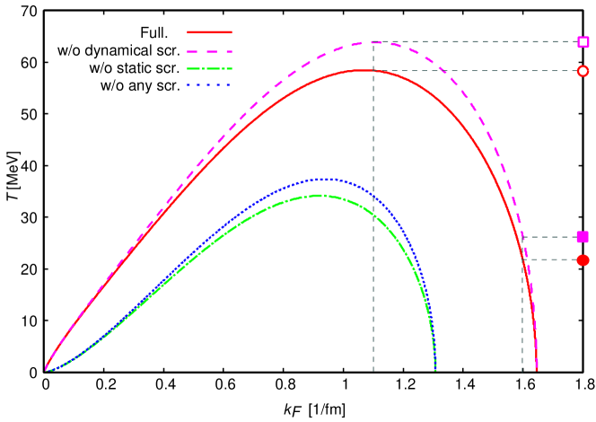
Figure 5: Magnetic phase diagram in the density-temperature plane. The solid, dashed, dash-dotted, dotted curves show the results for the full expression Eq. (60), the one without the $T^{2}\ln T$ term, without the $\kappa\ln\kappa$ term, and without the $T^{2}\ln T$ and $\kappa\ln\kappa$ terms in Eq. (60). The open (filled) circle indicates the Curie temperature at $k_{F}=1.1(1.6)$ fm^-1 while the squares show those when we disregard the $T^{2}\ln T$ dependence.

\psfrag{A}{\small$\delta\chi_{T^{2}}^{-1}$}\psfrag{B}{\small$\delta\chi_{T^{2}\ln T}^{-1}$}\psfrag{D}{\small$-\chi_{M}^{-1}(0)$}\psfrag{F}{$\delta\chi^{-1}_{M}(T)$}\psfrag{G}{}\includegraphics[width=208.13574pt]{Figure6left.eps}

\psfrag{A}{\small$\delta\chi_{T^{2}}^{-1}$}\psfrag{B}{\small$\delta\chi_{T^{2}\ln T}^{-1}$}\psfrag{D}{\small$-\chi_{M}^{-1}(0)$}\psfrag{F}{$\delta\chi^{-1}_{M}(T)$}\psfrag{G}{}\includegraphics[width=208.13574pt]{Figure6right.eps}

Figure 6: Contributions to the magnetic susceptibility. The left panel shows the result for $k_{F}=1.1$ fm^-1 and the right one is for $k_{F}=1.6$ fm^-1 in the unit of $\chi_{\rm Pauli}=1$. The solid, dashed, dash-dotted, and dotted curves show $\delta\chi^{-1}_{M}(T)$, $\delta\chi_{T^{2}}^{-1}$, $\delta\chi_{T^{2}\ln T}^{-1}$, and $-\chi_{M}^{-1}(0)$ respectively. The circles(squares) indicate the critical(Curie) temperatures including(ignoring) the $T^{2}\ln T$ dependence. $\delta\chi^{-1}_{T^{2}(T^{2}\ln T)}$ means the $T^{2}$ ($T^{2}\ln T$) term in the magnetic susceptibility, Eq. (60).

The maximum Curie temperature $T_{c}^{\rm max}$ is around $60$MeV, which is achieved at $k_{F}\simeq 1.1$fm^-1. Note that this is still low temperature, since $T_{c}^{\rm max}/k_{F}\ll 1$. Thus our low-temperature expansion is legitimate over all points on the critical curve. One of interesting phenomenological implications may be related to thermal evolution of magnetars; during the supernova expansions temperature rises up to several tens MeV, which is so that ferromagnetic phase transition may occur in the initial cooling stage to produce huge magnetic field.

In Fig.6, we plot the contributions to the magnetic susceptibility from the temperature independent, $T^{2}$ , and $T^{2}\ln T$ terms for $k_{F}=1.1$ fm^-1 and $k_{F}=1.6$ fm^-1. We represent the $T^{2}$ and $T^{2}\ln T$ term in Eq. (60) by $\delta\chi_{T^{2}}^{-1}$ and $\delta\chi_{T^{2}\ln T}^{-1}$ respectively. Compare the contributions from the two temperature-dependent terms. In either of the cases, the $T^{2}$ term is dominated over the $T^{2}\ln T$ term except at extremely low temperature. At sufficiently low temperature, the $T^{2}\ln T$ term should exceed the $T^{2}$ term, although we cannot see such a situation in Fig.6. Now, we estimate the reversal temperature, $T_{rev}$, at which $\delta\chi_{T^{2}}^{-1}$ starts to exceed $\delta\chi_{T^{2}\ln T}^{-1}$. This temperature is easily obtained from Eq. (59),

$$T_{rev} =\Lambda\exp\left[-\frac{12\pi^{2}}{C_{f}g^{2}u_{F}}\left(1+\frac{2k_{F}^{2}m^{2}+m^{4}}{2k_{F}^{4}+k_{F}^{2}m^{2}+m^{4}}\right)\right]$$

$$=T_{rev,c}\exp\left[-\frac{12\pi^{2}}{C_{f}g^{2}u_{F}}\left(\frac{2k_{F}^{2}m^{2}+m^{4}}{2k_{F}^{4}+k_{F}^{2}m^{2}+m^{4}}\right)\right]$$ (62)

where $T_{rev,c}$ is the reversal temperature of the specific heat, at which the $T$ term and the $T\ln T$ term in the specific heat or the entropy, Eq.(53) are equal in magnitude. $T_{rev}$ is quite low for the densities we are interested in.(For example, $T_{rev}=O(0.01)$MeV for $k_{F}=1.1$ fm^-1 and $T_{rev}=O(1)$ MeV for $k_{F}=1.6$ fm^-1.) As is shown in Fig. 6, the $T^{2}\ln T$ dependence is too important to neglect, although the reversal temperature of the magnetic susceptibility is quite low.

5 Summary and concluding remarks

We have discussed some magnetic aspects of quark matter by evaluating the magnetic susceptibility at finite temperature based on QCD, where the screening effects for gluons are taken into account. Different from the usual FLT, we cannot use the low temperature expansion because the quasi-particle energy have an anomalous term on the Fermi surface. Carefully studying the temperature effects, we have found that the magnetic properties of QCD exhibit interesting features reflecting the gauge interaction: the dynamic screening of the transverse gluon field gives an anomalous $T^{2}\ln T$ contribution to the magnetic susceptibility [38], while the contribution by the longitudinal gluons is almost temperature independent due to the Debye mass. It may be interesting to recall that the dynamic screening has no effect but the static screening gives the term proportional to $M_{D}^{2}\ln M_{D}^{-1}$ at $T=0$[20] with the Debye mass $M_{D}$; $M_{D}$ works as an infrared (IR) cutoff to remove the infrared singularity in the quasi-particle interaction exchanging the longitudinal gluons, while the IR singularity still remains in the quasi-particle interaction due to the transverse gluons. At finite temperature, the energy transfer of order $T$ is allowed among the quasi-particles in the vicinity of the Fermi surface, so that temperature itself plays a role of the IR cutoff through the dynamic screening for the quasi-particle interaction. The logarithmic temperature dependence appears in the magnetic susceptibility as a novel non-Fermi-liquid effect, and its origin is the same as in the well-known $T\ln T$ dependence of the specific heat [24, 28, 29, 30, 31, 32, 33]. The dynamic screening also gives $\ln T$ terms for the spin-asymmetric Landau-Migdal parameter as well as the density of states on the Fermi surface as the leading-order contribution, but they exactly cancel each other in the formula of the magnetic susceptibility. Hence $T^{2}\ln T$ term becomes the leading-order contribution. The anomalous $T^{2}\ln T$ term works against the magnetic instability, as well as the usual $T^{2}$ term.

We demonstrated how the temperature effects work by drawing the magnetic phase diagram on the density-temperature plane. We also figured out the role of the non-Fermi-liquid effect in the phase diagram. We have seen that the $T^{2}\ln T$ term should have a sizable effect on the magnetic phase diagram in the temperature-density plane .

We have seen some relations between the microscopic many-body calculation and the FLT; the Landau-Migdal parameter $f_{1}^{s}$ or $F_{1}^{s}$ for the spin symmetric interaction is closely connected with the quark self-energy and thereby the renormalization factor $z_{+}(k_{F})$. It diverges at $T=0$ due to the transverse mode, but another divergence coming from the spin dependent interaction cancel it to give a finite result for the magnetic susceptibility. At finite temperature all the Landau-Migdal parameters become finite. We have also derived the temperature dependence of the chemical potential within FLT to get the same result as that given by the microscopic calculation.

The magnetic susceptibility is a powerful tool to study not only the magnetic properties of QCD but also the magnetic transition in quark matter. However, it only gives the information about the curvature at the origin of the effective potential (free energy) with respect to magnetization. We have discussed the magnetic phase diagram in QCD, assuming that the magnetic transition is of the second order or the weakly first order. If the phase transition is of the first-order, we must explore the global behavior of the effective potential. The critical density or the critical (Curie) temperature then would be larger than that in this paper. It would be an interesting possibility to be further investigated[43, 44].

Here we have only considered the Fock exchange interaction in a perturbation method to reveal the interesting features of the magnetic properties within gauge theories. We have used a rather large coupling constant to demonstrate the specific features of the magnetic phase transition and the magnetic phase diagram, referring to the bag model parameter, where the color magnetic interaction gives a spin-spin interaction to split the mass degeneracy, e.g. for nucleon and $\Delta$ isobar. To be more realistic, we must take into account the non-perturbative effects, since some non-perturbative effects, like instantons [43, 45], are still relevant at low and intermediate densities. Actually some part of the mass splitting should be attributed to such non-perturbative effects, which in turn affect the magnetic properties of quark matter. Although the coupling constant should be small in this case, the non-Fermi- liquid behavior still survives as a qualitative effect.

In high-density QCD color superconductivity (CSC) has been extensively studied by many authors [46]. We have completely discarded its possibility in this paper to concentrate in the magnetic properties. It would be interesting to study the interplay of superconductivity and magnetism in quark matter. A first attempt in this direction has been already done [9], but more studies are needed to this end.

Finally, it should be worth noting that magnetic properties of QCD or its magnetic instability may be related to physics of compact stars, especially magnetars [11] or primordial magnetic field in early universe, where one may expect the QCD phase transition [47]. Our phase diagram may have a direct relevance to the thermal evolution of magnetars; the evolution path can be plotted on the temperature-density plane, and it may traverse the critical line in the initial cooling stage just after the supernova explosion.

Appendix A

The matrix elements for two quarks with $\zeta$ and $\zeta^{\prime}$

$$M^{00} = {\rm tr}[\gamma^{0}\rho(k,\zeta)\gamma^{0}\rho(q,\zeta^{\prime})],$$

$$M^{ij} = {\rm tr}[\gamma^{i}\rho(k,\zeta)\gamma^{j}\rho(q,\zeta^{\prime})],$$ (63)

can be easily evaluated. A straightforward manipulation, using Eq. (3), gives

$$M^{00} = \frac{1}{4m^{2}}\left\{2k_{0}q_{0}-k\cdot q+m^{2}+(m^{2}-q\cdot k)(2a_{0}b_{0}-a\cdot b)\right.$$ (64)

$$- \left.\left[-2a_{0}q_{0}k\cdot b+2k_{0}q_{0}a\cdot b-2k_{0}b_{0}a\cdot q+k\cdot ba\cdot q\right]\right\},$$

and

$$M^{ij} = \frac{1}{4m^{2}}\left\{(1-a\cdot b)\widehat{k^{i}q^{j}}+(m^{2}-k\cdot q)\widehat{a^{i}b^{j}}+a\cdot q\widehat{k^{i}b^{j}}+b\cdot k\widehat{q^{i}a^{j}}\right.$$ (65)

$$+\left.g^{ij}\left[(m^{2}-k\cdot q)(1-a\cdot b)-k\cdot bq\cdot a\right]\right\},$$

with a symbol, $\widehat{k^{i}q^{j}}=k^{i}q^{j}+k^{j}q^{i}$, where the spin vector $a_{\mu}$ is given by Eq. (2) and similarly $b_{\mu}$ by ${\bf b}=\mbox{\boldmath$\zeta$}^{\prime}+{\bf q}(\mbox{\boldmath$\zeta$}^{\prime}\cdot{\bf q})/m(E_{q}+m),b^{0}={\bf q}\cdot\mbox{\boldmath$\zeta$}^{\prime}/m$.

Appendix B

We present here some relations between the self-energy $\Sigma_{+}$ and the Landau parameter. The Fermi-liquid interaction of OGE is calculated at $T=0$ as

$$\left.f_{{\bf k}\zeta,{\bf q}\zeta^{\prime}}\right|_{|{\bf k}|=|{\bf q}|=k_{F}}=-\frac{m^{2}N_{c}^{-1}C_{f}g^{2}}{E_{F}^{2}}\lim_{\omega\rightarrow\mu}\left[-M^{00}{D}_{l}(\omega-\mu,{\bf k}-{\bf q})+M^{ii}{D}_{t}(\omega-\mu,{\bf k}-{\bf q})\right],$$ (66)

where the matrix elements $M^{\mu\nu}$ are given in Appendix A, and the propagator renders

$${D}_{l}(\omega-\mu,{\bf k}-{\bf q})\simeq-\frac{1}{2k_{F}^{2}(1-\cos\theta_{\widehat{{\bf k}{\bf q}}}+\kappa)},$$ (67)

for the longitudinal gluons with $\kappa$ being the parameter in terms of the Debye mass, $\kappa=M_{D}^{2}/2k_{F}^{2}=\sum_{f}m_{D,f}^{2}/2k_{F}^{2}$. The propagator for the transverse gluons renders

$$\left.D_{t}(\omega-\mu,{\bf k}-{\bf q})\right|_{|{\bf k}|=|{\bf q}|=k_{F}}\simeq-\frac{1}{2k_{F}^{2}\left[1-\cos\theta_{\widehat{{\bf k}{\bf q}}}+ic^{3/2}\frac{\omega-\mu}{(1-\cos\theta_{\widehat{{\bf k}{\bf q}}})^{1/2}}\right]},$$ (68)

with $c^{3}\equiv\frac{1}{8k_{s}^{6}}\left(\sum_{f}\frac{\pi m_{D,f}^{2}u_{F,f}}{4}\right)^{2}$ in the soft-gluon limit, $|\omega-\mu|/\mu\ll 1$.

It is rather easy to see the contributions to the Landau-Migdal parameters from the longitudinal gluons, since they have no IR singularity. For the spin-averaged interaction, we have

$$f^{s}_{l}=-N_{c}^{-1}C_{f}g^{2}\frac{m^{2}}{E_{F}^{2}}\lim_{\epsilon_{\bf k}\rightarrow\mu}M^{00s}D_{l}(\epsilon_{\bf k}-\mu,{\bf k}-{\bf q})|_{|{\bf k}|=|{\bf q}|=k_{F}},$$ (69)

with

$$M^{00s}=\frac{1}{4}\sum_{\zeta,\zeta^{\prime}}M^{00}=\frac{1}{4m^{2}}\left(E_{F}^{2}+k_{F}^{2}\cos\theta_{\widehat{{\bf k}{\bf q}}}+m^{2}\right).$$ (70)

Accordingly the Landau-Migdal parameter, $f_{l;1}^{s}$ reads

$$f_{l;1}^{s} \equiv \frac{3}{2}\int d(\cos\theta_{\widehat{{\bf k}{\bf q}}})\cos\theta_{\widehat{{\bf k}{\bf q}}}f^{s}_{l}$$ (71)

$$= -\frac{3N_{c}^{-1}C_{f}g^{2}}{8E_{F}^{2}k_{F}^{2}}\left[\kappa k_{F}^{2}+2E_{F}^{2}\right]\left[(1+\kappa)I_{0}(\kappa)-1\right].$$

Using the relation of the density of state near the Fermi surface and the spin-averaged Landau-Migdal parameter [7], we find $1/3f_{l;1}^{s}$ contributes to $N(0)$ at $T=0$. Since there is little temperature dependence for the short-range interaction, we have $N_{l}(T)\simeq N_{c}k_{F}E_{F}/(3\pi^{2})f_{l;1}^{s}$. Recalling Eq. (22), we can make sure that the longitudinal contribution is implicitly included in $\Sigma_{+}$ through $\Delta^{\rm reg}$.

For the transverse gluons, we must carefully calculate the Landau-Migdal parameters, since they never receive the static screening but the dynamic one due to the Landau damping. Generally $D_{t}$ includes the imaginary part proportional to the squared Debye mass, but it only gives a higher-order contribution. The real part of the Fermi-liquid interaction now reads

$$\left.f_{t;{\bf k}\zeta,{\bf q}\zeta^{\prime}}\right|_{|{\bf k}|=|{\bf q}|=k_{F}}\sim-\frac{N_{c}^{-1}C_{f}g^{2}m^{2}}{E_{F}^{2}}\lim_{\omega\rightarrow\mu}\left[M^{ii}{\rm Re}D_{t}(\omega-\mu,{\bf k}-{\bf q})\right]_{|{\bf k}|=|{\bf q}|=k_{F}}.$$ (72)

For the spin-dependent Landau parameter $\bar{f}^{a}_{t}$ we have already seen in §3 that

$$\bar{f}^{a}_{t}\sim\frac{C_{f}N_{c}^{-1}g^{2}}{12E_{F}^{2}}\lim_{\epsilon_{\bf k}\rightarrow\mu}{\rm ln}|\epsilon_{\bf k}-\mu|$$ (73)

as a leading-order contribution. For the spin averaged interaction,

$$f^{s}_{t}=-N_{c}^{-1}C_{f}g^{2}\frac{m^{2}}{E_{F}^{2}}\lim_{\epsilon_{\bf k}\rightarrow\mu}M^{iis}{\rm Re}D_{t}(\epsilon_{\bf k}-\mu,{\bf k}-{\bf q})|_{|{\bf k}|=|{\bf q}|=k_{F}},$$ (74)

with

$$M^{iis}\equiv\frac{1}{4}\sum_{\zeta,\zeta^{\prime}}M^{ii}=\frac{k_{F}^{2}}{2m^{2}}\left[1+\frac{1}{2}(1-\cos\theta_{\widehat{{\bf k}{\bf q}}})\right].$$ (75)

One can see that the relevant Landau parameter $f_{t;1}^{s}$ also contains ${\rm ln}|\epsilon_{\bf k}-\mu|$ due to the angular integral. $f_{t;1}^{s}$ is defined by

$$f_{t;1}^{s}\equiv\frac{3}{2}\int d(\cos\theta_{\widehat{{\bf k}{\bf q}}})\cos\theta_{\widehat{{\bf k}{\bf q}}}f^{s}_{t}.$$ (76)

Consider the integral,

$$\hskip 10.00002pt\int_{-1}^{1}d(\cos\theta_{\widehat{{\bf k}{\bf q}}})\cos\theta_{\widehat{{\bf k}{\bf q}}}{\rm Re}D_{t}M^{iis}$$

$$=-\frac{1}{8m^{2}}\int_{0}^{2}(1-x)(2+x)\frac{x^{2}}{x^{3}+{\tilde{c}}^{3}}dx$$

$$=-\frac{1}{8m^{2}}\left[\frac{2}{3}\ln\left|\frac{8+{\tilde{c}}^{3}}{{\tilde{c}}^{3}}\right|-4+\frac{{\tilde{c}}}{6}\ln\left|\frac{(2+\tilde{c})^{3}}{8+{\tilde{c}}^{3}}\right|\right.+\frac{{\tilde{c}}}{\sqrt{3}}\left(\tan^{-1}\frac{4-{\tilde{c}}}{\sqrt{3}{\tilde{c}}}+\frac{\pi}{6}\right)$$

$$\hskip 120.00018pt+\frac{{\tilde{c}}^{2}}{6}\ln\left|\frac{8+{\tilde{c}}^{3}}{(2+{\tilde{c}})^{3}}\right|+\left.\frac{{\tilde{c}}^{2}}{\sqrt{3}}\left({\rm tan}^{-1}\frac{4-{\tilde{c}}}{\sqrt{3}{\tilde{c}}}+\frac{\pi}{6}\right)\right],$$ (77)

with $\tilde{c}=c(\epsilon_{\bf k}-\mu)^{2/3}$. For a small $|\epsilon_{\bf k}-\mu|$, it reads

$$=-\frac{1}{8m^{2}}\left[-2{\rm ln}\left(\frac{c(\epsilon_{\bf k}-\mu)^{2/3}}{2}\right)-4+O((\epsilon_{\bf k}-\mu)^{4/3})\right].$$ (78)

Thus the leading-order contribution to $f_{t;1}^{s}$ is eventually given by

$$f_{t;1}^{s}\equiv\lim_{\epsilon_{\bf k}\rightarrow\mu}f_{t;1{\bf k}}^{s},$$ (79)

with $f_{t;1{\bf k}}^{s}\sim-\frac{C_{f}g^{2}N_{c}^{-1}}{4E_{F}^{2}}{\rm ln}|\epsilon_{\bf k}-\mu|$ or

$$F_{t;1}^{s}\equiv N(0)f_{t;1}^{s}\simeq-\frac{C_{f}g^{2}k_{F}}{4\pi^{2}E_{F}}\lim_{\epsilon_{\bf k}\rightarrow\mu}{\rm ln}|\epsilon_{\bf k}-\mu|,$$ (80)

up to $O(g^{2})$. Comparing Eq. (80) with Eq. (22), we can see

$$F_{t;1}^{s}=\lim_{\epsilon_{\bf k}\rightarrow\mu}\left.\frac{\partial{\rm Re}\Sigma_{+}(\omega)}{\partial\omega}\right|_{\omega=\epsilon_{\bf k}},$$ (81)

in the leading order.

Consider the renormalization factor on the Fermi surface, which measures a discontinuity of the momentum distribution of the bare particles [6, 26, 27]. We find

$$z_{+}(k_{F})\simeq\left(1+\frac{1}{3}F_{t;1}^{s}\right)^{-1}=0.$$ (82)

The Fermi velocity is given by

$$v_{F}^{-1}\simeq\frac{\mu}{k_{F}}\left(1+\frac{1}{3}F_{t;1}^{s}\right)\rightarrow\infty.$$ (83)

Moreover, one can see that

$$v_{F}=\frac{k_{F}}{\mu}z_{+}(k_{F}).$$ (84)

In the non-relativistic version, this relation is nothing but the relation between the effective mass $m^{*}$ and the renormalization factor $z_{+}(k_{F})$, $m^{*}=z_{+}^{-1}(k_{F})$.

At $T\neq 0$, the contribution of $f_{t;1}^{s}$ to $N(T)$ can be estimated by evaluating

$$-2N_{c}\int\frac{d^{3}k}{(2\pi)^{3}}\frac{\partial n(\epsilon_{\bf k})}{\partial\epsilon_{\bf k}}\frac{f_{t;1{\bf k}}^{s}}{3}=-\frac{C_{f}g^{2}u_{F}}{12\pi^{2}}\ln T,$$ (85)

which is reduced to $1/3F^{s}_{t;1}$ at $T=0$. Thus we can see that the $\ln T$ term in Eq. (30) is just given by the Landau-Migdal parameter $f_{t;1}^{s}$.

Appendix C

Here we derive Eq. (30). Substituting Eq. (22) into Eq. (26) and changing the variable $\omega$ by the dimensionless one $y$ through $\omega-\mu=yT$, we have

$$N(T)\simeq\frac{N_{c}}{\pi^{2}}\int_{-\infty}^{\infty}dyk(\mu+yT)E_{k(\mu+yT)}\left(1-\left.\frac{{\rm Re}\Sigma_{+}(\omega)}{\partial\omega}\right|_{\omega=\mu+yT}\right)\frac{e^{y}}{(e^{y}+1)^{2}},$$ (86)

where we put $(\epsilon_{0}-\mu)/T\rightarrow-\infty$ in the lower limit of the integral. Now we expand the each term in the integrand to find the leading-order contribution at low temperature. We thus have

$$1-\left.\frac{\partial{\rm Re}\Sigma_{+}(\omega)}{\partial\omega}\right|_{\omega=\mu+yT}\simeq 1-\frac{C_{f}g^{2}u_{F}}{12\pi^{2}}\ln\left(\frac{T}{\Lambda}\right),$$ (87)

and

$$k(\mu+yT)E_{k(\mu+yT)}\simeq k_{s}E_{s}+\frac{E_{F}(2k_{F}^{2}-m^{2})}{2k_{F}^{3}}y^{2}T^{2}\left(1-\frac{C_{f}g^{2}u_{F}}{6\pi^{2}}\ln\left(\frac{T}{\Lambda}\right)\right),$$ (88)

in the integrand, where the odd-power terms of $y$ is discarded since they never contribute to the integral with respect to $y$. Finally we have

$$\!\!\!\!\!\!\!\!\!\!\!N(T)\simeq\frac{N_{c}}{\pi^{2}}\int_{-\infty}^{\infty}dy\!\!\!\!\!\!\! \!\!\!\!\!\!\left[k_{s}E_{s}\left(1-\frac{C_{f}g^{2}u_{F}}{12\pi^{2}}\ln\left(\frac{T}{\Lambda}\right)\right)\right.$$ (89)

$$\!\!\!+\!\!\!\left.\frac{E_{F}(2k_{F}^{2}-m^{2})}{2k_{F}^{3}}y^{2}T^{2}\left(\!\!1-\frac{C_{f}g^{2}u_{F}}{4\pi^{2}}\ln\left(\frac{T}{\Lambda}\right)\right)\right]\frac{e^{y}}{(e^{y}+1)^{2}}.$$

The integral in Eq. (89) is easy to give Eq. (30).

References

• [1] O. Philipsen, arXiv:0710.1217
• [2] P. Braun-Munzinger and J. Stachel, Nature 448 (2007) 302.
• [3] For recent reviews,
F. Weber, Prog. in Part. and Nucl. Phys. 54 (2005) 193.
D. Page and S. Reddy, Ann. Rev. of Nucl. and Part. Sci. 56 (2006) 327.
J.M. Lattimer and M. Prakash, Phys. Rep. 442 (2007) 109.
• [4] T. Schaefer, arXiv:hep-ph/0509068.
P. Braun-Munzinger and J. Wambach, arXiv:0801.4256.
• [5] G. Baym and C.J. Pethick, Landau Fermi-Liquid Theory (WILEY-VCH, 2004).
A.A. Abrikosov, L.P. Gorkov and I.E. Dzaloshinski, Methods of Quantum Field Theory in Statistical Physics (Prentice-Hall. Inc., 1963).
A.B. Migdal, Theory of finite Fermi systems (Intersci. Pub., 1967).
• [6] P. Noziéres, Theory of Interacting Fermi Systems (Westview Press,1997).
D. Pines and P. Noziéres, The Theory of Quantum Liquids (Perseus books Pub., 1999).
• [7] G. Baym and S.A. Chin, Nucl. Phys. A262 (1976) 527.
• [8] T. Tatsumi, Phys. lett. B489 (2000) 280.
T. Tatsumi, E. Nakano and K. Nawa, Dark Matter, p.39 (Nova Science Pub., New York, 2006).
• [9] E. Nakano, T. Maruyama and T. Tatsumi, Phys. Rev. D68 (2003) 105001.
T. Tatsumi, E. Nakano and T. Maruyama, Prog. Theor. Phys. Suppl. 153 (2004) 190.
T. Tatsumi, T. Maruyama and E. Nakano, Superdense QCD Matter and Compact Stars, p.241 (Springer, 2006).
• [10] A. Niegawa, Prog. Theor. Phys. 113 (2005) 581.
• [11] P.M. Woods and C. Thompson, Soft gamma ray repeaters and anomalous X-ray pulsars:magneter candidates, Compact stellar X-ray sources, 2006, 547.
A.K. Harding and D. Lai, Rep. Prog. Phys. 69 (2006) 2631.
• [12] F. Bloch, Z. Phys. 57 (1929) 545;
• [13] C. Herring, Exchange Interactions among Itinerant Electrons: Magnetism IV (Academic press, New York, 1966)
K. Yoshida, Theory of magnetism (Springer, Berlin, 1998).
• [14] T. Moriya, Spin Fluctuations in Itinerant Electron Magnetism (Springer, 1985)
• [15] D.K. Hong, Phys. Lett. B473 (2000) 118; Nucl. Phys. B582 (2000) 451.
• [16] T. Schäfer and K. Schwenzer, Phys. Rev. D70 (2004) 054007; 114037.
• [17] S. Hands, Phys. Rev. D69 (2004) 014020.
• [18] J.I. Kapusta, Finite-temperature field theory (Cambridge U. Press, 1993).
M. Le Bellac, Thermal Field Theory (Cambridge U. Press, 1996).
• [19] T. Tatsumi, Exotic States of Nuclear Matter (World Sci., 2008) 272.
• [20] T. Tatsumi and K. Sato, Phys. Lett. B663 (2008) 322.
• [21] K.A. Brueckner and K. Sawada, Phys. Rev. 112 (1957) 328.
B.S. Shastray, Phys. Rev. Lett. 38 (1977) 449.
• [22] R. Shanker, Rev. Mod. Phys. 66 (1994) 129.
• [23] C. Nayak and F. Wilczek, Nucl. Phys. B430 (1994) 534.
J. Polchinski, Nucl. Phys. B422 (1994) 617.
• [24] D. Boyanovsky and H.J. de Vega, Phys. Rev. D63 (2001) 034016; 114028.
• [25] C. Manuel and Le Bellac, Phys. Rev. D55 (1997) 3215.
C. Manuel, Phys. Rev. D62 (2000) 076009.
• [26] J.M. Luttinger and J.C. Ward, Phys. Rev. 118 (1960) 1417.
J.M. Luttinger, Phys. Rev. 119 (1960) 1153.
• [27] J.M. Luttinger, Phys. Rev. 121 (1961) 942.
• [28] T. Holstein, R.E. Norton and P. Pincus, Phys. Rev. B8 (1973) 2649.
• [29] M.Yu. Reizer, Phys. Rev. B40 (1989) 11572; B44 (1991) 5476.
• [30] J. Gan and E. Wong, Phys. Rev. Lett. 71 (1993) 4226.
• [31] S. Chakravarty, R.E. Norton and O.F. Syljuasen, Phys. Rev. Lett. 74 (1995) 1423.
• [32] A. Ipp, A. Gerhold and A. Rebhan, Phys. Rev. D69 (2004) 011901.
A. Gerhold, A. Ipp and A. Rebhan, Phys. Rev, D70 (2004) 105015; PoS (JHW2005) 013.
• [33] A. Gerhold and A. Rebhan, Phys. Rev. D71 (2005) 085010.
• [34] D.T. Son, Phys. Rev. D59 (1999) 094019.
• [35] T. Schäfer and F. Wilczek, Phys. Rev. D60 (1999) 114033.
• [36] W.E. Brown, J.T. Liu and H. Ren, Phys. Rev. D61 (2000) 114012; D62(2000) 054013.
• [37] Q. Wang and D.H. Rischke, Phys. Rev. D65 (2002) 054005.
• [38] T. Tatsumi and K. Sato, Phys. Lett. B672 (2009) 132.
• [39] C. Itzykson and J.-B. Zuber, Quantum Field Theory (McGraw-Hill Inc., 1980).
• [40] V.B. Berestetsii, E.M. Lifshitz and L.P. Pitaevsii,
Relativistic Quantum Theory (Pergamon Press, 1971).
• [41] K. Ohnishi, M. Oka and S. Yasui, Phys. Rev. D76 (2007) 097501.
• [42] T.A. DeGrand, R.L. Jaffe, K. Johnson and J. Kiskis, Phys. Rev. D12 (1975) 2060.
• [43] M. Inui, H. Kohyama and A. Niegawa, arXiv:0709.2204.
• [44] K. Pal, S. Biswas and A.K. Dutt-Mazumder, arXiv:0809.0404.
• [45] S.-il Nam, H.-Y. Ryu, M.M. Musakhanov and H.-C. Kim, arXiv:0804.0056.
• [46] For a recent review, M.G. Alford, K. Rajagopal, T. Schaefer, A. Schmit, arXiv:0709.4635.
• [47] D. Boyanovsky, H.J. de Vega, D.J. Schwarz, Ann. Rev. Nucl. Part. Sci. (2006) 441.