A Unified Approach to Distance-Two Colouring
of Graphs on Surfaces

Abstract

In this paper we introduce the notion of $\Sigma$-colouring of a graph $G$: For given subsets $\Sigma(v)$ of neighbours of $v$, for every $v\in V(G)$, this is a proper colouring of the vertices of $G$ such that, in addition, vertices that appear together in some $\Sigma(v)$ receive different colours. This concept generalises the notion of colouring the square of graphs and of cyclic colouring of graphs embedded in a surface. We prove a general result for graphs embeddable in a fixed surface, which implies asymptotic versions of Wegner’s and Borodin’s Conjecture on the planar version of these two colourings. Using a recent approach of Havet et al., we reduce the problem to edge-colouring of multigraphs, and then use Kahn’s result that the list chromatic index is close to the fractional chromatic index.

Our results are based on a strong structural lemma for graphs embeddable in a fixed surface, which also implies that the size of a clique in the square of a graph of maximum degree $\Delta$ embeddable in some fixed surface is at most $\frac{3}{2}\,\Delta$ plus a constant.

1 Introduction

Most of the terminology and notation we use in this paper is standard and can be found in any text book on graph theory (such as [2] or [8]). All our graphs and multigraphs will be finite. A multigraph can have multiple edges; a graph is supposed to be simple. We will not allow loops. The vertex and edge set of a graph $G$ are denoted by $V(G)$ and $E(G)$, respectively (or just $V$ and $E$, if the graph $G$ is clear from the context).

Given a graph $G$, the chromatic number of $G$, denoted $\chi(G)$, is the minimum number of colours required so that we can properly colour its vertices using those colours. If we colour the edges of $G$, we get the chromatic index, denoted $\chi^{\prime}(G)$. The list chromatic number or choice number $\mathit{ch}(G)$ is the minimum value $k$ such that if we give each vertex $v$ of $G$ a list $L(v)$ of at least $k$ colours, then we can find a proper colouring in which each vertex gets assigned a colour from its own private list. The list chromatic index $\mathit{ch}^{\prime}(G)$ is defined analogously for edges.

The square $G^{2}$ of a graph $G$ is the graph with vertex set $V(G)$, with an edge between any two different vertices that have distance at most two in $G$. A proper vertex colouring of the square of a graph can also be seen as a vertex colouring of the original graph satisfying:

$\bullet$vertices that are adjacent receive different colours, and

$\bullet$vertices that have a common neighbour receive different colours.

Another way to formulate these conditions is as ‘vertices at distance one or two must receive different colours’. This is why the name distance-two colouring is also used in the literature.

In this paper we consider a colouring concept that generalises the concept of colouring the square of a graph, but that also can be used to study different concepts such as cyclic colouring of plane graphs (definition will be given later).

For a vertex $v\in V$, let $N(v)$ (or $N_{G}(v)$ if we want to specify the graph under consideration) be the set of vertices adjacent to $v$. Suppose that for each vertex $v\in V$, we are given a subset $\Sigma(v)\subseteq N(v)$ of its neighbourhood. We call such a collection a $\Sigma$-system for $G$.

A $\Sigma$-colouring of $G$ is an assignment of colours to the vertices of $G$ so that:

$\bullet$vertices that are adjacent receive different colours, and

$\bullet$vertices that appear together in some $\Sigma(v)$ receive different colours.

When additionally each vertex $v$ has its own list $L(v)$ of colours from which its colour must be chosen, we talk about a list $\Sigma$-colouring.

We denote by $\chi(G;\Sigma)$ the minimum number of colours required for a $\Sigma$-colouring to exist. Its list variant is denoted by $\mathit{ch}(G;\Sigma)$, and is defined as the minimum integer $k$ such that for each assignment of a list $L(v)$ of at least $k$ colours to vertices $v\in V$, there exists a proper $\Sigma$-colouring of $G$ in which all vertices are assigned colours from their own lists.

Notice that we trivially have $\chi(G)=\chi(G;\varnothing)$ and $\chi(G^{2})=\chi(G;N_{G})$; and the same relations holds for the list variant ($\varnothing$ assigns the empty set to each vertex).

We define the width of a $\Sigma$-system of $G$ as $\Delta(G;\Sigma)=\max_{v\in V}|\Sigma(v)|$. It is clear that we always need at least $\Delta(G;\Sigma)+1$ colours in a proper $\Sigma$-colouring. In the case $\Sigma\equiv N_{G}$, there exist plenty of graphs $G$ that require $O(\Delta(G)^{2})$ colours (where $\Delta(G)=\Delta(G;N_{G})$ is the usual maximum degree of $G$). But for planar graphs, it is known that a constant times $\Delta(G)$ colours is enough (even for list colouring). We will take a closer look at this in Subsection 1.1 below.

Following Wegner’s Conjecture on colouring the square of planar graphs (see also next subsection), we propose the following conjecture.

Conjecture 1.1

There exist constants $c_{1},c_{2}$ and $c_{3}$ such that for all planar graphs $G$ and any $\Sigma$-system for $G$, we have

$$\chi(G;\Sigma)\> \leq\>\bigl{\lfloor}\tfrac{3}{2}\,\Delta(G;\Sigma)\bigr{\rfloor}+c_{1};$$

$$\mathit{ch}(G;\Sigma)\> \leq\>\bigl{\lfloor}\tfrac{3}{2}\,\Delta(G;\Sigma)\bigr{\rfloor}+c_{2};$$

$$\mathit{ch}(G;\Sigma)\> \leq\>\bigl{\lfloor}\tfrac{3}{2}\,\Delta(G;\Sigma)\bigr{\rfloor}+1,\qquad\qquad\text{if $\Delta(G;\Sigma)\geq c_{3}$}.$$

If $\Sigma\equiv\varnothing$ (hence $\Delta(G;\Sigma)=0$), then the Four Colour Theorem implies that the smallest possible value for $c_{1}$ is four; while the fact that planar graphs are always 5-list colourable but not always 4-list colourable, shows that the smallest possible value for $c_{2}$ is five.

Our main result is that Conjecture 1.1 is asymptotically correct: $\mathit{ch}(G;\Sigma)\leq\frac{3}{2}\,\Delta(G;\Sigma)+o\bigl{(}\Delta(G;\Sigma)\bigr{)}$. In fact, we can prove this asymptotic result holds for general surfaces.

Theorem 1.2

For every surface $S$ and any real $\varepsilon>0$, there exists a constant $\beta_{S,\varepsilon}$ such that the following holds for all $\beta\geq\beta_{S,\varepsilon}$. If $G$ is a graph embeddable in $S$, with a $\Sigma$-system of width at most $\beta$, then $\mathit{ch}(G;\Sigma)\leq\bigl{(}\frac{3}{2}+\varepsilon\bigr{)}\,\beta$.

A trivial lower bound for the (list) chromatic number of a graph $G$ is the clique number $\omega(G)$, the maximum size of a clique in $G$. For graphs with a $\Sigma$-system, we can define the following related concept. A $\Sigma$-clique is a subset $C\subseteq V$ such that every two different vertices in $C$ are adjacent or appear together in some $\Sigma(v)$. Denote by $\omega(G;\Sigma)$ the maximum size of a $\Sigma$-clique in $G$. Then we trivially have $\mathit{ch}(G;\Sigma)\geq\omega(G;\Sigma)$, and so Theorem 1.2 means that for a graph $G$ embeddable in some fixed surface $S$, we have $\omega(G;\Sigma)\leq\frac{3}{2}\,\Delta(G;\Sigma)+o(\Delta(G;\Sigma))$.

But in fact, the structural result we use to prove Theorem 1.2 fairly easily gives $\omega(G;\Sigma)\leq\frac{3}{2}\,\Delta(G;\Sigma)+O(1)$.

Theorem 1.3

For every surface $S$, there exist constants $\beta_{S}$ and $\gamma_{S}$ such that the following holds for all $\beta\geq\beta_{S}$. If $G$ is a graph embeddable in $S$, with a $\Sigma$-system of width at most $\beta$, then every $\Sigma$-clique in $G$ has size at most $\frac{3}{2}\,\beta+\gamma_{S}$.

The main steps in the proof of Theorem 1.2 can be found in Section 2. The proof relies on two technical lemmas; the proofs of those can be found in Section 3. After that we use one of those lemmas to provide the relatively short proof of Theorem 1.3 in Section 4. In Section 5 we discuss some of the aspects of our work and discuss open problems related to (list) $\Sigma$-colouring of graphs. The final section provides some background regarding the proof by Kahn [17] of the asymptotical equality of the fractional chromatic index and the list chromatic index of multigraphs. A more general result, contained implicitly in Kahn’s work, is of crucial importance to our proof in this paper.

In the next two subsections, we discuss two special consequences of these results. These special versions of Theorems 1.2 and 1.3 also show that the term $\frac{3}{2}\,\beta$ is best possible.

But before presenting these applications, a remark is in order. In an earlier version of this paper, we gave our results in terms of $(A,B)$-colourings. For a graph $G$ and vertex sets $A,B\subseteq V$ (not necessarily disjoint), an $(A,B)$-colouring of $G$ is a colouring of the vertices in $B$ such that adjacent vertices, and vertices with a common neighbour in $A$, receive different colours.

There is an obvious way to translate an $(A,B)$-colouring problem into a $\Sigma$-colouring problem: For $v\in A$ set $\Sigma(v)=N_{G}(v)\cap B$, and for $v\notin A$ set $\Sigma(v)=\varnothing$. Note that after this translation we are required to colour all vertices, not just those in $B$. But the vertices outside $B$ do not appear in any $\Sigma(v)$, hence colouring them for a graph embeddable in a fixed surface requires at most a constant number of colours.

On the other hand, it is easy to construct instances of $\Sigma$-colouring problems for which there is no obvious translation to an $(A,B)$-colouring problem. In that sense, we feel justified in considering $\Sigma$-colouring as a more general concept.

1.1 Colouring the Square of Graphs

Recall that the square of a graph $G$, denoted $G^{2}$, is the graph with the same vertex set as $G$ and with an edge between any two different vertices that have distance at most two in $G$. If $G$ has maximum degree $\Delta$, then a vertex colouring of its square will need at least $\Delta+1$ colours, and the greedy algorithm shows that it is always possible to find a colouring of $G^{2}$ with $\Delta^{2}+1$ colours. Cages of diameter two, such as the 5-cycle, the Petersen graph and the Hoffman-Singleton graph (see, e.g., [2, page 84]), show that there exist graphs that in fact require $\Delta^{2}+1$ colours.

Regarding the chromatic number of the square of a planar graph, Wegner [33] posed the following conjecture (see also the book of Jensen and Toft [14, Section 2.18]), suggesting that for planar graphs far less than $\Delta^{2}+1$ colours suffice.

Conjecture 1.4 (Wegner [33])

For a planar graph $G$ of maximum degree $\Delta$, $\chi(G^{2})\>\leq\>\left\{\begin{array}[]{ll}7,&\text{if $\Delta=3$,}\\ \Delta+5,&\text{if $4\leq\Delta\leq 7$,}\\ \bigl{\lfloor}\frac{3}{2}\,\Delta\bigr{\rfloor}+1,&\text{if $\Delta\geq 8$.}\end{array}\right.$

Wegner also gave examples showing that these bounds would be tight. For $\Delta\geq 8$ even, these examples are sketched in Figure 1(a).

(a)

(b)

Figure 1: (a) A planar graph $G$ with maximum degree $\Delta=2k$ and $\omega(G^{2})=\chi(G^{2})=3k+1=\bigl{\lfloor}\frac{3}{2}\,\Delta\bigr{\rfloor}+1$.
(b) A planar graph $H$ with maximum face order $\Delta^{*}=2k$ and $\chi^{*}(H)=3k=\bigl{\lfloor}\frac{3}{2}\,\Delta^{*}\bigr{\rfloor}$ (see Subsection 1.2).

The graph in the picture has maximum degree $2k$ and yet all the vertices except $z$ are pairwise adjacent in its square. Hence to colour these $3k+1$ vertices, we need at least $3k+1=\frac{3}{2}\,\Delta+1$ colours. Note that the same arguments also show that the graph $G$ in the picture has $\omega(G^{2})=\frac{3}{2}\,\Delta+1$.

Kostochka and Woodall [19] conjectured that for the square of any graph, the chromatic number equals the list chromatic number. This conjecture and Wegner’s one together imply the conjecture that for planar graphs $G$ with $\Delta\geq 8$, we have $\mathit{ch}(G^{2})\leq\bigl{\lfloor}\frac{3}{2}\,\Delta\bigr{\rfloor}+1$.

The first upper bound on $\chi(G^{2})$ for planar graphs in terms of $\Delta$, $\chi(G^{2})\leq 8\Delta-22$, was implicit in the work of Jonas [15]. This bound was later improved by Wong [34] to $\chi(G^{2})\leq 3\Delta+5$ and then by Van den Heuvel and McGuinness [13] to $\chi(G^{2})\leq 2\Delta+25$. Better bounds were then obtained for large values of $\Delta$. It was shown by Agnarsson and Halldórsson [1] that for $\Delta\geq 750$ we have $\chi(G^{2})\leq\lceil\frac{9}{5}\,\Delta\rceil+1$; the same bound was proved for $\Delta\geq 47$ by Borodin et al. [4]. Finally, the best known upper bound so far has been obtained by Molloy and Salavatipour [25]: $\chi(G^{2})\leq\lceil\frac{5}{3}\,\Delta\rceil+78$. As mentioned in [25], the constant 78 can be reduced for sufficiently large $\Delta$. For example, it was improved to 24 when $\Delta\geq 241$.

Since $\mathit{ch}(G^{2})=\mathit{ch}(G;N_{G})$ (i.e., $\Sigma(v)=N_{G}(v)$ for all $v\in V$), as an immediate corollary of Theorem 1.2 we obtain.

Corollary 1.5

Let $S$ be a fixed surface. Then the square of every graph $G$ embeddable in $S$ and of maximum degree $\Delta$ has list chromatic number at most $\frac{3}{2}\,\Delta+o(\Delta)$.

In fact, the same asymptotic upper bound as in Corollary 1.5 can be proved even for larger classes of graphs. Additionally, a stronger conclusion on the colouring is possible. For the following result, we assume that colours are integers, which allows us to talk about the ‘distance’ $|\alpha_{1}-\alpha_{2}|$ between two colours $\alpha_{1},\alpha_{2}$.

Theorem 1.6 (Havet, Van den Heuvel, McDiarmid & Reed [10])

Let $k$ be a fixed positive integer. The square of every $K_{3,k}$-minor free graph $G$ of maximum degree $\Delta$ has list chromatic number (and hence clique number) at most $\frac{3}{2}\,\Delta+o(\Delta)$. Moreover, given lists of this size, there is a proper colouring in which the colours on every pair of adjacent vertices of $G$ differ by at least $\Delta^{1/4}$.

Note that planar graphs do not have a $K_{3,3}$-minor. In fact, for every surface $S$, there is a constant $k$ such that no graph embeddable in $S$ has $K_{3,k}$ as a minor. This shows that Theorem 1.6 is stronger than our Corollary 1.5. On the other hand, Theorem 1.6 gives a weaker bound for the clique number than the one we obtain in Corollary 1.7 below.

Both Corollary 1.5 and Theorem 1.6 can be applied to $K_{4}$-minor free graphs, since these graphs are planar and do not have $K_{3,3}$ as a minor. But the best possible bounds for this class are actually known. Lih, Wang and Zhu [21] showed that the square of $K_{4}$-minor free graphs with maximum degree $\Delta$ has chromatic number at most $\bigl{\lfloor}\frac{3}{2}\,\Delta\bigr{\rfloor}+1$ if $\Delta\geq 4$ and $\Delta+3$ if $\Delta=2,3$. The same bounds, but then for the list chromatic number of $K_{4}$-minor free graphs, were proved by Hetherington and Woodall [12].

Regarding the clique number of the square of graphs, we get the following corollary of Theorem 1.3.

Corollary 1.7

Let $S$ be a fixed surface. Then the square of every graph $G$ embeddable in $S$ and of maximum degree $\Delta$ has clique number at most $\frac{3}{2}\,\Delta+O(1)$.

From the proof of Theorem 1.3, it can be deduced that the square of a planar graph with maximum degree $\Delta\geq 11616$ has clique number at most $\frac{3}{2}\,\Delta+76$.

Very recently, this was improved by the following result.

Theorem 1.8 (Cohen & Van den Heuvel [7])

For a planar graph $G$ of maximum degree $\Delta\geq 41$, we have $\omega(G^{2})\leq\bigl{\lfloor}\frac{3}{2}\,\Delta\bigr{\rfloor}+1$.

Apart from the bound $\Delta\geq 41$, this theorem is best possible, as is shown by the same graphs that show that Wegner’s Conjecture 1.4 is best possible for $\Delta\geq 8$ (see also Figure 1(a)).

1.2 Cyclic Colourings of Embedded Graphs

Given a surface $S$ and a graph $G$ embeddable in $S$, we denote by $G^{S}$ that graph with a prescribed embedding in $S$. If the surface $S$ is the sphere, we talk about a plane graph $G^{P}$. The order of a face of $G^{S}$ is the number of vertices in its boundary; the maximum order of a face of $G^{S}$ is denoted by $\Delta^{*}(G^{S})$.

A cyclic colouring of an embedded graph $G^{S}$ is a vertex colouring of $G$ such that any two vertices in the boundary of the same face have distinct colours. The minimum number of colours required in a cyclic colouring of an embedded graph is called the cyclic chromatic number $\chi^{*}(G^{S})$. This concept was introduced for plane graphs by Ore and Plummer [26], who also proved that for a plane graph $G^{P}$, we have $\chi^{*}(G^{P})\leq 2\Delta^{*}$. Borodin [3] (see also Jensen and Toft [14, page 37]) conjectured the following.

Conjecture 1.9 (Borodin [3])

For a plane graph $G^{P}$ of maximum face order $\Delta^{*}$, we have $\chi^{*}(G^{P})\leq\bigl{\lfloor}\frac{3}{2}\,\Delta^{*}\bigr{\rfloor}$.

The bound in this conjecture is best possible. Consider the plane graph depicted in Figure 1(b): It has $3k$ vertices and has three faces of order $\Delta^{*}=2k$. Since all pairs of vertices have a face they are both incident with, we need $3k=\bigl{\lfloor}\frac{3}{2}\,\Delta^{*}\bigr{\rfloor}$ colours in a cyclic colouring.

Borodin [3] also proved Conjecture 1.9 for $\Delta^{*}=4$. For general values of $\Delta^{*}$, the original bound $\chi^{*}(G^{P})\leq 2\Delta^{*}$ of Ore and Plummer [26] was improved by Borodin et al. [6] to $\chi^{*}(G^{P})\leq\bigl{\lfloor}\frac{9}{5}\,\Delta^{*}\bigr{\rfloor}$. The best known upper bound in the general case is due to Sanders and Zhao [29]: $\chi^{*}(G^{P})\leq\bigl{\lceil}\frac{5}{3}\,\Delta^{*}\bigr{\rceil}$.

Although Wegner’s and Borodin’s Conjectures seem to be closely related, nobody has ever been able to bring to light a direct connection between them. Most of the results approaching these conjectures use the same ideas, but up until this point no one had proved a general theorem implying both a result on the colouring of the square and a result on the cyclic colouring of plane graphs (let alone on embedded graphs).

In order to show that our Theorem 1.2 provides an asymptotically best possible upper bound for the cyclic chromatic number for a graph $G$ with some fixed embedding $G^{S}$, we need some extra notation. For each face $f$ of $G^{S}$, add a vertex $x_{f}$. For any face $f$ of $G^{S}$ and any vertex $v$ in the boundary of $f$, add an edge between $v$ and $x_{f}$, and denote by $G_{F}$ the graph obtained from $G^{S}$ by this construction. Note that the vertex set of $G_{F}$ consists of $V(G)$ and all the new vertices $x_{f}$, for $f$ a face of $G^{S}$. Define a $\Sigma$-system $\Sigma_{F}$ for $G_{F}$ as follows: For each vertex $v\in V(G)$, let $\Sigma_{F}(v)=\varnothing$. For each vertex $x_{f}$, let $\Sigma_{F}(x_{f})$ be all the neighbours of $x_{f}$. Observe that a (list) $\Sigma_{F}$-colouring of $G_{F}$ colours the vertices of $G$ in a way required for a cyclic (list) colouring of $G^{S}$, and that $\Delta(G_{F};\Sigma_{F})=\Delta^{*}(G^{S})$.

(Note that in fact we have $\chi^{*}(G^{S})\leq\chi(G_{F},\Sigma_{F})\leq\chi^{*}(G^{S})+1$. To get the second inequality, start with a cyclic colouring of $G^{S}$, add one extra colour, and colour all the vertices $x_{f}$ with that colour. Similar inequalities hold for the list version.)

Using the upper bound on $\chi^{*}(G^{S})$, we get the following corollary of Theorem 1.2.

Corollary 1.10

Let $S$ be a fixed surface. Every embedding $G^{S}$ of a graph $G$ of maximum face order $\Delta^{*}$ has cyclic list chromatic number at most $\frac{3}{2}\,\Delta^{*}+o(\Delta^{*})$.

For an embedded graph $G^{S}$, the cyclic clique number $\omega^{*}(G^{S})$ is the maximum size of a set $C\subseteq V$ such that every two vertices in $C$ have some face they are both incident with. Note that the plane graph depicted in Figure 1(b) satisfies $\omega^{*}(G^{P})=3k=\bigl{\lfloor}\frac{3}{2}\,\Delta^{*}\bigr{\rfloor}$. This shows that the following corollary of Theorem 1.3 is best possible, up to the constant term.

Corollary 1.11

Let $S$ be a fixed surface. Every embedded graph $G^{S}$ of maximum face order $\Delta^{*}$ has cyclic clique number at most $\frac{3}{2}\,\Delta^{*}+O(1)$.

For plane graphs, the proof of Theorem 1.3 guarantees that a plane graph $G^{P}$ of maximum face order $\Delta^{*}\geq 11616$ has cyclic clique number at most $\frac{3}{2}\,\Delta^{*}+76$.

2 Proof of Theorem 1.2

Our goal in this section is to show that for all surfaces $S$ and any $\varepsilon>0$, if we take $\beta$ large enough (depending on $S$ and $\varepsilon$), then for every graph $G=(V,E)$ embeddable in $S$, every choice of $\Sigma(v)\subseteq N_{G}(v)$ with $|\Sigma(v)|\leq\beta$ for all $v\in V$, and every assignment $L(v)$ of at least $\bigl{(}\frac{3}{2}+\varepsilon\bigr{)}\,\beta$ colours to all $v\in V$, there is a list $\Sigma$-colouring of $G$ where each vertex receives a colour from its own list. In other words, we want an assignment $c(v)$ for each $v\in V$ such that:

$\bullet$for all $v\in V$, we have $c(v)\in L(v)$;

$\bullet$for all $u,v\in V$ with $uv\in E$, we have $c(u)\neq c(v)$; and

$\bullet$for all $u,v\in V$ for which there is a $t\in V$ with $u,v\in\Sigma(t)$, we have $c(u)\neq c(v)$.

Before we present the actual proofs, we recall some of the important terminology, notation and facts concerning embeddings of graph in surfaces.

2.1 Graphs in Surfaces

In this subsection, we give some background about graphs embedded in a surface. For more details, the reader is referred to [23]. Here, by a surface we mean a compact 2-dimensional surface without boundary. An embedding of a graph $G$ in a surface $S$ is a drawing of $G$ on $S$ so that all vertices are distinct, and every edge forms a simple arc connecting in $S$ the vertices it joins, so that the interior of every edge is disjoint from other vertices and edges. A face of this embedding (or just a face of $G$, for short) is an arc-wise connected component of the space obtained by removing the vertices and edges of $G$ from the surface $S$.

We say that an embedding is cellular if every face is homeomorphic to an open disc in $\mathbb{R}^{2}$.

A surface can be orientable or non-orientable. The orientable surface $\mathbb{S}_{h}$ of genus $h$ is obtained by adding $h\geq 0$ ‘handles’ to the sphere; while the non-orientable surface $\mathbb{N}_{k}$ of genus $k$ is formed by adding $k\geq 1$ ‘cross-caps’ to the sphere. The genus $\mathbf{g}(G)$ and non-orientable genus $\widetilde{\mathbf{g}}(G)$ of a graph $G$ is the minimum $h$ and the minimum $k$, resp., such that $G$ has an embedding in $\mathbb{S}_{h}$, resp. in $\mathbb{N}_{k}$.

The following result will allow us to suppose that a graph $G$ with known genus $\mathbf{g}(G)$ or non-orientable genus $\widetilde{\mathbf{g}}(G)$ can be assumed to be embedded in a cellular way.

Lemma 2.1 ([23, Propositions 3.4.1 and 3.4.2])

(i)Every embedding of a connected graph $G$ in $\mathbb{S}_{\mathbf{g}(G)}$ is cellular.

(ii)If $G$ is a connected graph different from a tree, then there is an embedding of $G$ in $\mathbb{N}_{\widetilde{\mathbf{g}}(G)}$ that is cellular.

The Euler characteristic $\chi(S)$ of a surface $S$ is $2-2h$ if $S=\mathbb{S}_{h}$, and $2-k$ if $S=\mathbb{N}_{k}$.

The basic result connecting all these concepts is Euler’s Formula: If $G$ is a graph with an embedding in $S$, with vertex set $V$, edge set $E$ and face set $F$, then

$$|V|-|E|+|F|\>\geq\>\chi(S).$$

Moreover, if the embedding is cellular, then we have equality in Euler’s Formula.

Finally, if $v$ is a vertex of a graph $G$ embedded in a surface $S$, then that embedding imposes two circular orders of the edges incident with $v$. Since we assume graphs to be simple, this corresponds to two circular orders of the neighbours of $v$. If $S$ is orientable, then we can consistently choose one of the two clockwise orders for all vertices; if $S$ is non-orientable, then such a choice is not possible. In our proofs that follow, it is not important that we can choose a consistent circular order; we only require that for each vertex $v$, there is at least one circular order of the neighbours around $v$.

If $u_{1},u_{2}$ are consecutive neighbours of $v$ (with respect to the chosen circular order), then there is a face that has the three vertices $u_{1},v,u_{2}$ in its boundary. That immediately gives the following observation.

Lemma 2.2

Let $G$ be a graph embedded in a surface $S$. Suppose $u_{1},u_{2}$ are consecutive neighbours of $v$ (with respect to the chosen circular order). Then the graph obtained by adding the edge $u_{1}u_{2}$ (if it is not already present) is still embeddable in $S$.

That observation has the following corollary.

Lemma 2.3

Let $G$ be a connected graph embedded in a surface $S$. If $G$ has more than three vertices and is edge-maximal with respect to being embeddable in $S$, then every vertex has degree at least three.

2.2 The First Steps

For $P,Q\subseteq V$, the set of edges between $P$ and $Q$ is denoted by $E(P,Q)$, and the number of edges between $P$ and $Q$ is denoted by $e(P,Q)$ (edges with both ends in $P\cap Q$ are counted twice).

For a graph $G$ with a $\Sigma$-system, and a vertex $v\in V$, we denote by $\sigma(v)$ the size of $\Sigma(v)$, i.e., $\sigma(v)=|\Sigma(v)|$. A $\Sigma$-neighbour of a vertex $v$ is a vertex $u\neq v$ such that either $u$ and $v$ are adjacent, or there is some $t\in V$ with $u,v\in\Sigma(t)$. Denote the number of $\Sigma$-neighbours of $v$ by $d^{\Sigma}(v)$. Note that we have

$$d^{\Sigma}(v)\>\leq\>d(v)+\!\!\sum_{t\text{ with }v\,\in\,\Sigma(t)}\!\!(\sigma(t)-1).$$

An important tool in our proof of Theorem 1.2 is the following technical structural result, Lemma 2.4. Before stating this lemma, we need a few extra definitions. For an integer $\zeta$, a special $\zeta$-pair is a pair $(X,Y)$ of disjoint subsets of vertices $X$ and $Y$ (possibly empty) with the following property:

         (i)Every vertex in $X$ has degree at least $\zeta+1$. Every vertex $y\in Y$ has degree four, is adjacent to exactly two vertices of $X$, and the remaining neighbours of $y$ have degree four as well.

Given a special $\zeta$-pair $(X,Y)$, for any $y\in Y$, let $X^{y}$ be the set of two neighbours of $y$ in $X$. For $W\subseteq X$, let $Y^{W}$ be the set of all vertices $y\in Y$ with $X^{y}\subseteq W$ (that is, the set of vertices of $Y$ having their two neighbours from $X$ in $W$).

A special $\zeta$-pair $(X,Y)$ is called very special if in addition the following condition holds:

         (ii)For all pairs of vertices $y,z\in Y$, if $y$ and $z$ are adjacent or have a common neighbour $w\notin X$, then $X^{y}=X^{z}$.

The general structure of a very special $\zeta$-pair is sketched in Figure 2.

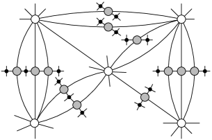
Figure 2: Sets $X$ (white vertices) and $Y$ (grey vertices) forming a very special 8-pair $(X,Y)$ in a graph. Neighbours of vertices of $Y$ not in $X$ are depicted as small black vertices, and the remaining vertices are not depicted for the sake of clarity.

With these definitions, our structural lemma can be stated as follows:

Lemma 2.4

Let $S$ be a fixed surface, set $\zeta_{S}^{*}=132\,(3-\chi(S))$, and let $G$ be a graph embeddable in $S$. If $G$ is edge-maximal with respect to being embeddable in $S$, then one of the following three properties holds.

(S1)Every vertex has degree at most $\zeta_{S}^{*}$.

(S2)There is a vertex of degree at most five with at most one neighbour of degree more than $\zeta_{S}^{*}$.

(S3)There exists a very special $\zeta_{S}^{*}$-pair $(X,Y)$ such that $X,Y$ are both non-empty and for all non-empty subsets $W\subseteq X$, the following inequality holds:

$$e(W,V\setminus Y)\>\leq\>e(W,Y\setminus Y^{W})+\zeta_{S}^{*}\,|W|.$$

Very informally, Lemma 2.4 states that a graph that is maximally embeddable in some fixed surface, either contains one of two fairly simple configurations, or it contains a structure that internally satisfies a specific density-type condition.

Structure (S3) is at the heart of the above lemma. Although its description might appear technical at first sight, it will be clear later that it is the exact kind of density condition needed in the proofs of Theorems 1.2 and 1.3.

The proof of Lemma 2.4 can be found in Subsection 3.1. Observe that the value we use for $\zeta_{S}^{*}$ is probably far from best possible. The important point, to our mind, is that it only depends on (the Euler characteristic of) the surface $S$.

We continue with a description how to apply the lemma to prove Theorem 1.2. Suppose the theorem is false. Then there is a surface $S$ and a real $\varepsilon>0$ such that for every $\beta_{S,\varepsilon}$ we can find $\beta\geq\beta_{S,\varepsilon}$ and a graph $G$, together with a $\Sigma$-system of width at most $\beta$, such that $\mathit{ch}(G;\Sigma)>\bigl{(}\frac{3}{2}+\varepsilon\bigr{)}\,\beta$. Set $\zeta_{S}^{*}=132\,(3-\chi(S))$ and $\beta_{S}^{*}=\tfrac{2}{3}\,(\zeta_{S}^{*})^{2}=11616\,(3-\chi(S))^{2}$. Note that, as $\chi(S)\leq 2$, this means $\zeta_{S}^{*}\geq 132$ and $\beta_{S}^{*}\geq 11616$.

We start by assuming $\beta\geq\beta_{S}^{*}$; later (at the end of Subsection 2.3) we will add some further lower bounds for $\beta$ that will depend on $\varepsilon$. With respect to this (yet to come) final choice of $\beta$, there exists a graph $G=(V,E)$ embeddable in $S$, together with a $\Sigma$-system of width at most $\beta$ and a list-assignment $L$ of at least $\bigl{(}\frac{3}{2}+\varepsilon\bigr{)}\,\beta$ colours to each vertex $v\in V$, such that $G$ has no $\Sigma$-colouring from these lists. Choose such a graph $G$ with the minimum number of vertices, and subject to this, with the maximum number of edges.

Certainly we can assume that $G$ is connected (otherwise one of the components will be a smaller counterexample). Also, since each vertex has a list of more than $\frac{3}{2}\,\beta\geq 17424$ colours, $G$ itself will have more than 17424 vertices.

Next we can assume that $G$ is edge-maximal with respect to being embeddable in $S$. Otherwise we can add a new edge $uv$ to $G$ so that the resulting graph $G_{1}$ is still embeddable in $S$, and set $\Sigma_{1}\equiv\Sigma$. It is clear that a list $\Sigma_{1}$-colouring of $G_{1}$ is also is a list $\Sigma$-colouring of $G$.

Fix some embedding of $G$ in $S$. We continue with applying Lemma 2.4 to $G$.

2.2.1 The structure from (S1) is present in $G$

This is the easiest case: If the degree of every vertex is at most $\zeta_{S}^{*}$, then the number of $\Sigma$-neighbours of any vertex is at most $\zeta_{S}^{*}+\zeta_{S}^{*}\cdot(\zeta_{S}^{*}-1)=(\zeta_{S}^{*})^{2}$. But the number of colours in each list $L(v)$ is at least $\bigl{(}\frac{3}{2}+\varepsilon\bigr{)}\,\beta>\frac{3}{2}\,\beta_{S}^{*}=(\zeta_{S}^{*})^{2}$. So a simple greedy colouring will do the job; contradicting that $G$ is a counterexample.

2.2.2 The structure from (S2) is present in $G$

So there is a vertex $v$ of degree at most five, and at most one of its neighbours has degree more than $\zeta_{S}^{*}$. Since $|V|\geq 17424$, by Lemma 2.3, $v$ has degree at least three. Hence it has a neighbour $u$ of degree at most $\zeta_{S}^{*}$. Form the graph $G_{2}$ by contracting $uv$ into a new vertex $w$ (remove multiple edges if they appear). Set $V_{2}=(V\setminus\{u,v\})\cup\{w\}$. Let $\Sigma_{2}(w)=(\Sigma(u)\cup\Sigma(v))\setminus\{u,v\}$. For a vertex $t\in V_{2}\setminus\{w\}$, if $\Sigma(t)$ contains $u$, then set $\Sigma_{2}(t)=(\Sigma(t)\setminus\{u,v\})\cup\{w\}$; otherwise, set $\Sigma_{2}(t)=\Sigma(t)\setminus\{v\}$. Finally, give $w$ the list of colours $L(w)=L(u)$. Note that $G_{2}$ is smaller than $G$ and is still embeddable in $S$. Moreover, for every $t\in V_{2}\setminus\{w\}$, we have $|\Sigma_{2}(t)|\leq|\Sigma(t)|\leq\beta$; while for $w$ we have $|\Sigma_{2}(w)|\leq d_{G}(u)+d_{G}(v)\leq 5+\zeta_{S}^{*}\leq\beta$.

So there exists a list $\Sigma_{2}$-colouring of $G_{2}$. We define a colouring of $G$ as follows: Every vertex different from $u$ and $v$ keeps its colour from the colouring of $G_{2}$. We give $u$ the colour given to $w$ in $G_{2}$. Finally, we observe that for $v$ we have

$$d^{\Sigma}(v)\>\leq\>d(v)+\!\!\!\sum_{t\text{ with }v\,\in\,\Sigma(t)}\!\!\!(\sigma(t)-1)\>\leq\>5+4\,(\zeta_{S}^{*}-1)+(\beta-1)\>=\>4\zeta_{S}^{*}+\beta\>\leq\>\tfrac{3}{2}\,\beta,$$

since $\beta\geq\tfrac{2}{3}\,(\zeta_{S}^{*})^{2}\geq 8\zeta_{S}^{*}$. Since $v$ has at least $\bigl{(}\frac{3}{2}+\varepsilon)\,\beta$ colours in its list, there exists a free colour for $v$, i.e., a colour different from the colour of all the vertices in conflict with $v$. We colour $v$ with such a free colour. By the construction of $G_{2}$ and $\Sigma_{2}$, it is easy to verify that this defines a list $\Sigma$-colouring of $G$, contradicting the choice of $G$ as a counterexample.

2.2.3 The structure from (S3) is present in $G$

Let $X$ and $Y$ be two non-empty disjoint subsets of $V$ such that the pair $(X,Y)$ is a very special $\zeta_{S}^{*}$-pair satisfying the condition of (S3). We can remove from $X$ any vertex not adjacent to any vertex in $Y$.

Claim 2.5

For all $y\in Y$, we have that if $X^{y}=\{x_{1},x_{2}\}$, then $y\in\Sigma(x_{1})\cap\Sigma(x_{2})$.

• Proof   Suppose we have $y\notin\Sigma(x_{1})$. Since $(X,Y)$ is special, $y$ has degree four, and it has a neighbour $u$ not in $X^{y}$ of degree four. We also have $d^{\Sigma}(y)\leq 4+2\cdot(4-1)+(\sigma(x_{2})-1)\leq 9+\beta$. By contracting the edge $uy$, we can argue similarly to Subsection 2.2.2 (with $y$ now playing the role of $v$) to obtain a contradiction.   $\Box$

In the remainder of this subsection we describe how to reduce this case to a list edge-colouring problem. More precisely, we first define a modification of the original graph $G$ into a smaller graph $G_{0}$ with vertex set $V\setminus Y$, inheriting a $\Sigma$-system from that of $G$, so that the minimality of $G$ as a counterexample implies that $G_{0}$ admits a $\Sigma$-colouring. This colouring then provides a partial $\Sigma$-colouring of $G$, giving a colour to every vertex outside $Y$. In order to extend this partial colouring to the whole graph, we define a multigraph whose edges are indexed by the vertices in $Y$, so that an edge-colouring of that multigraph is exactly the extension of the $\Sigma$-colouring to $Y$ we are looking for. In the next subsection we then describe how Kahn’s approach to prove that the list chromatic index is asymptotically equal to the fractional chromatic index, can be used to conclude the proof of Theorem 1.2.

To define $G_{0}$, we divide the vertices of $Y$ into three parts according to their number of neighbours outside $X\cup Y$. Let $Y^{\prime}$ be the set of vertices in $Y$ with no neighbour outside $X\cup Y$. Consider first the graph $G[V\setminus Y^{\prime}]$ induced on the set of vertices outside $Y^{\prime}$. For each vertex $y\in Y^{\prime}$, add an edge between its two neighbours $\{x_{1},x_{2}\}=X^{y}$, if those are not already joined by an edge, and remove $y$ from $\Sigma(x_{1})$ and $\Sigma(x_{2})$. Also, add $x_{1}$ to $\Sigma(x_{2})$ and $x_{2}$ to $\Sigma(x_{1})$. Note that after these changes, $\Sigma(x_{1})$ and $\Sigma(x_{2})$ cannot be larger than before (since, by Claim 2.5, $y\in\Sigma(x_{i})$ for $i=1,2$).

For any vertex $y\in Y\setminus Y^{\prime}$ with a unique neighbour $u$ outside $X\cup Y$, contract the edge $yu$ (remove multiple edges if they appear), and, by an abuse of the notation, call the new vertex $u$ again. For the two vertices $x_{1}$ and $x_{2}$ in $X^{y}$, remove $y$ from $\Sigma(x_{1})$ and $\Sigma(x_{2})$. For the vertex $u$ itself, let $\Sigma(u)$ be equal to the set of all its neighbours.

And, finally, for any vertex $y\in Y\setminus Y^{\prime}$ with exactly two neighbours $u$ and $u^{\prime}$ outside $X\cup Y$, contract the edge $yu$ (remove multiple edges if they appear), and, by an abuse of the notation, call the new vertex $u$ again. For the two vertices $x_{1}$ and $x_{2}$ in $X^{y}$, remove $y$ from $\Sigma(x_{1})$ and $\Sigma(x_{2})$. Add $u$ to $\Sigma(u^{\prime})$ and remove $y$ from $\Sigma(u^{\prime})$ (if it was in this set). For the vertex $u$ itself, let $\Sigma(u)$ be equal to the set of all its neighbours. Note that $u^{\prime}$ has degree at most four in $G$, hence certainly $|\Sigma(u^{\prime})|\leq\beta$.

The graph obtained after the modifications described above is denoted by $G_{0}$, and the resulting sets by $\Sigma_{0}(v)$, $v\in V(G_{0})$. Note that, by our abuse of the notation, $G_{0}$ has the vertex set $V_{0}=V\setminus Y$. Next we observe that a vertex $u$ of $G$ outside $X\cup Y$ that was adjacent to a vertex $y\in Y$ (and hence may have been involved in one or more contractions) has degree four in $G$. Since vertices in $Y$ have degree four as well, each contraction increases the degree by at most two. So in $G_{0}$, such a vertex $u$ has degree at most twelve, hence we certainly have $|\Sigma_{0}(u)|\leq\beta$. By the construction above, we saw that for every other vertex $v\in V_{0}$, we also have $|\Sigma_{0}(v)|\leq|\Sigma(v)|\leq\beta$ or $|\Sigma_{0}(v)|\leq d_{G_{0}}(v)\leq\beta$.

By its construction, $G_{0}$ is embeddable in $S$. Also by construction, and the remarks above, it is easy to verify the following statement.

Claim 2.6

If $u,v\in V_{0}$ are adjacent in $G$, then $u,v$ are adjacent in $G_{0}$. If $u,v\in V_{0}$ and there is a $t\in V$ with $u,v\in\Sigma(t)$, then $u,v$ are either adjacent in $G_{0}$, or there is a $t_{0}\in V_{0}$ with $u,v\in\Sigma(t_{0})$.

For each vertex $v\in V_{0}$ set $L_{0}(v)=L(v)$. Since $Y\neq\varnothing$, by the minimality of $G$, the graph $G_{0}$ admits a list $\Sigma_{0}$-colouring $c_{0}$ with respect to the list assignment $L_{0}$.

We now transform this colouring into a partial list $\Sigma$-colouring of $G$ with respect to the original list assignment $L$, by just setting $c(v)=c_{0}(v)$ for each vertex $v\in V_{0}=V\setminus Y$. By Claim 2.6, this is indeed a good partial $\Sigma$-colouring of all the vertices of $V\setminus Y$ in $G$. The difficult part of the proof is to show that $c$ can be extended to $Y$.

By assumption, at the beginning every vertex in $Y$ has a list of at least $\bigl{(}\frac{3}{2}+\varepsilon\bigr{)}\,\beta$ available colours. For each vertex $y$ in $Y$, let us remove from $L(y)$ the colours which are forbidden for $y$ according to the partial $\Sigma$-colouring $c$ of $G$. In the worst case, these forbidden colours are exactly the colours of the vertices of $V\setminus Y$ at distance at most two from $y$.

Let us define the multigraph $H$ as follows: $H$ has vertex set $X$. And for each vertex $y\in Y$ we add an edge $e_{y}$ between the two neighbours of $y$ in $X$ (in other words, between the two vertices in $X^{y}$). Note that this process may produce multiple edges. We associate a list $L(e_{y})$ to $e_{y}$ in $H$ by taking the list of $y$ obtained after removing the set of forbidden colours for $y$ from the original list $L(y)$.

In what follows, following the usual terminology for multigraphs, we denote by $d_{H}(x)$ the degree of the vertex $x$ in the multigraph $H$, i.e., the number of edges incident with $x$ in $H$. By Claim 2.5, we have $N_{G}(x)\cap Y\subseteq\Sigma(x)$ for every $x\in X$, which guarantees $d_{H}(x)\leq\sigma(x)$.

We now prove the following lemma.

Lemma 2.7

A list edge-colouring for $H$, with the list assignment $L$ defined as above, provides an extension of $c$ to a list $\Sigma$-colouring of $G$ by giving to each vertex $y\in Y$ the colour of the edge $e_{y}$ in $H$.

• Proof   This follows since the pair $(X,Y)$ is very special: For every two vertices $y,z\in Y$, if $y$ and $z$ are adjacent or have a common neighbour $w\notin X$, then $X^{y}=X^{z}$. This proves that the two vertices adjacent in $Y$ or with a common neighbour not in $X$ define parallel edges in $H$ and so will have different colours. If two vertices $y_{1}$ and $y_{2}$ of $Y$ have a common neighbour in $X$, $e_{y_{1}}$ and $e_{y_{2}}$ will be adjacent in $H$ and so will get different colours. Since we have already removed from the list of vertices in $Y$ the set of forbidden colours (defined by the colours of the vertices in $V\setminus Y$), there will be no conflict between the colours of a vertex in $Y$ and a vertex in $V\setminus Y$. We conclude that the edge-colouring of $H$ will provide an extension of $c$ to a list $\Sigma$-colouring of $G$.   $\Box$

The following lemma provides a lower bound on the size of $L(e)$ for the edges $e$ in $H$.

Lemma 2.8

Let $e=x_{1}x_{2}$ be an edge in $H$. Then we have

$$|L(e)|\>\geq\>\bigl{(}\tfrac{3}{2}+\varepsilon\bigr{)}\,\beta-(\sigma(x_{1})-d_{H}(x_{1}))-(\sigma(x_{2})-d_{H}(x_{2}))-10.$$

• Proof   Let $y$ be the vertex in $Y$ such that $e=e_{y}$. By the definition of $H$, $X^{y}=\{x_{1},x_{2}\}$. Let $Z$ be the set of vertices in $V\setminus X$ adjacent to $y$ in $G$. Then, since $(X,Y)$ is a special $\zeta_{S}^{*}$-pair, $|Z|\leq 2$ and $|N_{G}(Z)\setminus Y|\leq 6$. The colours that are possibly forbidden for $y$ are the colours of $\{x_{1},x_{2}\}$, plus the colours of vertices in $(Z\cup N_{G}(Z))\setminus Y$, plus the colours of vertices in $(\Sigma(x_{1})\setminus Y)\cup(\Sigma(x_{2})\setminus Y)$ (note that these colours all come from the vertices outside $Y$). The number of vertices in these three sets add up to at most $10+(\sigma(x_{1})-d_{H}(x_{1}))+(\sigma(x_{2})-d_{H}(x_{2}))$. The lemma follows.   $\Box$

We finish this subsection by applying Lemma 2.4 in order to obtain information on the density of subgraphs in $H$, which we will need in the next subsection. Recall that for all non-empty subsets $W\subseteq X$, $Y^{W}$ denotes the set of vertices $y\in Y$ with $X^{y}\subseteq W$ (that is, the set of vertices of $Y$ having their two neighbours from $X$ in $W$). By (S3), we have for all non-empty $W\subseteq X$,

$$e_{G}(W,V\setminus Y)\>\leq\>e_{G}(W,Y\setminus Y^{W})+\zeta_{S}^{*}\,|W|.$$

This inequality has the following interpretation in $H$.

Lemma 2.9

For all non-empty subsets $W\subseteq X({}=V(H)\,)$, we have

$$\sum_{w\,\in\,W}(\sigma(w)-d_{H}(w))\>\leq\>e_{H}(W,X\setminus W)+\zeta_{S}^{*}\,|W|.$$

• Proof   First note that $\sum\limits_{w\,\in\,W}(\sigma(w)-d_{H}(w))\leq\sum\limits_{w\,\in\,W}(d_{G}(w)-d_{H}(w))=e_{G}(W,V\setminus Y)$. We also have $e_{G}(W,Y\setminus Y^{W})=e_{H}(W,X\setminus W)$. Combining these two observations with the formula in (S3) immediately gives the required inequality.   $\Box$

At this point, our aim will be to apply Kahn’s approach to the multigraph $H$ with the list assignment $L$, to prove the existence of a proper list edge-colouring for $H$. This is described in the next subsection.

We summarise the properties we assume are satisfied by the multigraph $H$ and the list assignment $L$ of the edges of $H$. For these conditions we just consider $\sigma(v)$ as an integer with certain properties, assigned to each vertex $v$ of $H$.

(H1)For all vertices $v$ in $H$, we have $d_{H}(v)\leq\sigma(v)\leq\beta$.

(H2)For all edges $e=uv$ in $H$, $|L(e)|\geq\bigl{(}\frac{3}{2}+\varepsilon\bigr{)}\,\beta-(\sigma(u)-d_{H}(u))-(\sigma(v)-d_{H}(v))-10$.

(H3)For all non-empty subsets $W\subseteq V(H)$, $\sum\limits_{w\,\in\,W}(\sigma(w)-d_{H}(w))\leq e_{H}(W,V(H)\setminus W)+\zeta_{S}^{*}\,|W|$, for some constant $\zeta_{S}^{*}$.

2.3 The Matching Polytope and Edge-Colourings

We briefly describe the matching polytope of a multigraph. More about this subject can be found in [30, Chapter 25].

Let $H$ be a multigraph with $m$ edges. Let $\mathcal{M}(H)$ be the set of all matchings of $H$, including the empty matching. For each $M\in\mathcal{M}(H)$, let us define the $m$-dimensional characteristic vector $\textbf{1}_{M}$ as follows: $\textbf{1}_{M}=(x_{e})_{e\in E(H)}$, where $x_{e}=1$ for an edge $e\in M$, and $x_{e}=0$ otherwise. The matching polytope of $H$, denoted $\mathcal{MP}(H)$, is the polytope defined by taking the convex hull of all the vectors $\textbf{1}_{M}$ for $M\in\mathcal{M}(H)$. Also, for any real number $\lambda$, we set $\lambda\,\mathcal{MP}(H)=\{\,\lambda\,x\mid x\in\mathcal{MP}(H)\,\}$.

Edmonds [9] gave the following characterisation of the matching polytope.

Theorem 2.10 (Edmonds [9])

A vector $\vec{x}=(x_{e})$ is in $\mathcal{MP}(H)$ if and only if $x_{e}\geq 0$ for all $x_{e}$ and the following two types of inequalities are satisfied:

$\bullet$For all vertices $v\in V(H)$, $\sum\limits_{e:\>\text{$v$ incident to $e$}}\!\!\!x_{e}\leq 1$;

$\bullet$for all subsets $W\subseteq V(H)$ with $|W|\geq 3$ and $|W|$ odd, $\sum\limits_{e\,\in\,E(W)}\!x_{e}\leq\tfrac{1}{2}\,(|W|-1).$

The significance of the matching polytope and its relation to list edge-colouring is indicated by the following important result.

Theorem 2.11 (Kahn [17])

For all real numbers $\delta,\nu$, $0<\delta<1$ and $\nu>0$, there exists a $\Delta_{\delta,\nu}$ such that for all $\Delta\geq\Delta_{\delta,\nu}$ the following holds. If $H$ is a multigraph and $L$ is a list assignment of colours to the edges of $H$ so that

$\bullet$$H$ has maximum degree at most $\Delta$;

$\bullet$for all edges $e\in E(H$), $|L(e)|\geq\nu\Delta$;

$\bullet$the vector $\vec{x}=(x_{e})$ with $x_{e}=\dfrac{1}{|L(e)|}$ for all $e\in E(H)$ is an element of $(1-\delta)\,\mathcal{MP}(H)$.

Then there exists a proper edge-colouring of $H$ where each edge gets a colour from its own list.

The theorem above is actually not explicitly stated this way in [17], but can be obtained from the appropriate parts of that paper. We give some further details about this in the final section of this paper.

The next lemma allows us to use Theorem 2.11 to complete the proof.

Lemma 2.12

Let $\beta$ and $\zeta$ be positive real numbers. Let $H$ be a multigraph with a map $\sigma:V(H)\rightarrow\mathbb{N}$, and a weighting $(b_{e})_{e\in E(H)}$ of the edges with positive real numbers satisfying the following three conditions:

(H1’)For all vertices $v$ in $H$, $d_{H}(v)\leq\sigma(v)\leq\beta$.

(H2’)For all edges $e=uv$ in $H$, $b_{e}\geq\bigl{(}\frac{3}{2}\,\beta+\tfrac{9}{2}\,\zeta\bigr{)}-(\sigma(u)-d_{H}(u))-(\sigma(v)-d_{H}(v))$.

(H3’)For all non-empty $W\subseteq V(H)$, $\sum\limits_{w\,\in\,W}(\sigma(w)-d_{H}(w))\leq e_{H}(W,V(H)\setminus W)+\zeta\,|W|$.

Then for all edges $e\in E(H)$, we have $b_{e}\geq\tfrac{1}{2}\,\beta$. And the vector $(1/b_{e})_{e\in E(H)}$ is in $\mathcal{MP}(H)$.

The proof of Lemma 2.12 will be given in Subsection 3.2. This lemma guarantees that for any $\varepsilon>0$, there exists a $\beta_{\varepsilon}$ such that for all $\beta\geq\beta_{\varepsilon}$, Theorem 2.11 can be applied to a multigraph $H$ with an edge list assignment $L$ satisfying properties (H1) – (H3) stated at the end of the previous subsection.

To see this, take $\delta_{\varepsilon}=\dfrac{\varepsilon}{3+2\varepsilon}$, so $0<\delta_{\varepsilon}<1$. In order to be able to apply Theorem 2.11, we want to prove the existence of $\beta_{\varepsilon,\zeta_{S}^{*}}$ such that for any $\beta\geq\beta_{\varepsilon,\zeta_{S}^{*}}$, the vector $\vec{x}=(x_{e})$, $x_{e}=\dfrac{1}{|L(e)|}$, is in $(1-\delta_{\varepsilon})\,\mathcal{MP}(H)$. Let $\zeta_{S}^{*}$ be the constant described in condition (H3). By condition (H2), we have for all $e=uv$ in $H$,

$$(1-\delta_{\varepsilon})\,|L(e)|\> \geq\>(1-\delta_{\varepsilon})\,\bigl{(}\bigl{(}\tfrac{3}{2}+\varepsilon\bigr{)}\,\beta-(\sigma(u)-d_{H}(u))-(\sigma(v)-d_{H}(v))-10\bigr{)}$$

$$\geq\>(1-\delta_{\varepsilon})\,\bigl{(}\tfrac{3}{2}+\varepsilon\bigr{)}\,\beta-(\sigma(u)-d_{H}(u))-(\sigma(v)-d_{H}(v))-10$$

$$=\>\bigl{(}\tfrac{3}{2}\,\beta+\tfrac{1}{2}\,\varepsilon\beta\bigr{)}-(\sigma(u)-d_{H}(u))-(\sigma(v)-d_{H}(v))-10.$$

Let $\beta_{\varepsilon,\zeta_{S}^{*}}=\dfrac{9\zeta_{S}^{*}+20}{\varepsilon}$. For $\beta\geq\beta_{\varepsilon,\zeta_{S}^{*}}$, we have

$$(1-\delta_{\varepsilon})\,|L(e)|\>\geq\>\bigl{(}\tfrac{3}{2}\,\beta+\tfrac{9}{2}\,\zeta_{S}^{*}\bigr{)}-(\sigma(u)-d_{H}(u))-(\sigma(v)-d_{H}(v)).$$

So by Lemma 2.12, taking $b_{e}=(1-\delta_{\varepsilon})\,|L(e)|$, the vector $\Bigl{(}\dfrac{x_{e}}{1-\delta_{\varepsilon}}\Bigr{)}_{e\in E(H)}$ is in $\mathcal{MP}(H)$. We infer that $\vec{x}\in(1-\delta_{\varepsilon})\,\mathcal{MP}(H)$.

Notice that the first conclusion of Lemma 2.12 means that $|L(e)|=\dfrac{b_{e}}{1-\delta_{\varepsilon}}>b_{e}\geq\tfrac{1}{2}\,\beta$ for all edges $e$ in $H$.

Now set $\beta_{S,\varepsilon}=\max\{\,\beta_{S}^{*},\,\beta_{\varepsilon,\zeta_{S}^{*}},\,\Delta_{\delta_{\varepsilon},1/2}\,\}$, where $\zeta_{S}^{*}=132\,(3-\chi(S))$, $\beta_{S}^{*}=\tfrac{2}{3}\,(\zeta_{S}^{*})^{2}$ (see Lemma 2.4 and the text after it), $\beta_{\varepsilon,\zeta_{S}^{*}}=\dfrac{9\zeta_{S}^{*}+20}{\varepsilon}$, $\delta_{\varepsilon}=\dfrac{\varepsilon}{3+2\varepsilon}$ (see above), and $\Delta_{\delta_{\varepsilon},1/2}$ is according to Theorem 2.11 (where $\Delta_{\delta_{\varepsilon},1/2}$ is chosen since we have $|L(e)|\geq\tfrac{1}{2}\,\beta$ for all $e\in E(H)$ (see above)). Assume $\beta\geq\beta_{S,\varepsilon}$. Then we can apply Theorem 2.11, which implies that the multigraph $H$ defined in Subsection 2.2 has a list edge-colouring corresponding to the list assignment $L$. Lemma 2.7 then implies that the colouring $c$ can be extended to a list $\Sigma$-colouring of the original graph $G$. This final contradiction completes the proof of Theorem 1.2.   

3 Proofs of the Main Lemmas

We use the terminology and notation from the previous sections.

3.1 Proof of Lemma 2.4

Let $S$ be a surface, set $\zeta_{S}^{*}=132\,(3-\chi(S))$, and let $G$ be a graph embeddable in $S$, so that $G$ is edge-maximal with respect to being embeddable in $S$.

From Lemma 2.2, we immediately obtain the following.

Claim 3.1

For any vertex $v$ and any two consecutive neighbours $u_{1},u_{2}$ of $v$ (consecutive with respect to the chosen circular order imposed by the embedding), we have $u_{1}u_{2}\in E(G)$.

Next we prove that we can assume $G$ has a cellular embedding in $S$. If $G$ is a tree, then every leaf will give a structure from (S2). So we can assume $G$ is not a tree. Assume $S$ is orientable with genus $h$. By the definition of $\mathbf{g}(G)$, we must have $\mathbf{g}(G)\leq h$, and hence $\chi(\mathbb{S}_{\mathbf{g}(G)})=2-2\,\mathbf{g}(G)\geq 2-2h=\chi(S)$. That also means that the constant in Lemma 2.4 satisfies $\zeta_{\mathbb{S}_{\mathbf{g}(G)}}^{*}\leq\zeta_{S}^{*}$. Hence if we prove the lemma assuming $G$ is embeddable in $\mathbb{S}_{\mathbf{g}(G)}$, then the lemma for $G$ embeddable in $S$ directly follows. So we can use Lemma 2.4 with the surface $\mathbb{S}_{\mathbf{g}(G)}$ instead of $S$, and by Lemma 2.1, we can use a cellular embedding of $G$ in $\mathbb{S}_{\mathbf{g}(G)}$.

If $S$ is non-orientable, then exactly the same argument can be applied, this time using the surface $\mathbb{N}_{\widetilde{\mathbf{g}}(G)}$ (and using the assumption that $G$ is not a tree).

We need some further notation and terminology. The set of faces of $G$ is denoted by $F$. Recall that since the embedding in $S$ is cellular, every face is homeomorphic to an open disk in $\mathbb{R}^{2}$. For such a face $f$, a boundary walk of $f$ is a walk consisting of vertices and edges as they are encountered when walking along the whole boundary of $f$, starting at some vertex. The degree of a face $f$, denoted $d(f)$, is the number of edges on the boundary walk of $f$. Note that this means that some edges may be counted more than once. The order of a face is the number of vertices in its boundary. We always have that the order of $f$ is at most $d(f)$.

Now suppose that $G$ does not contain any of the structures (S1) or (S2). In order to prove Lemma 2.4, we only need to prove that $G$ contains structure (S3). In other words, we need to prove that $G$ contains a very special $\zeta_{S}^{*}$-pair $(X,Y)$ with $X$ and $Y$ non-empty which satisfies the inequality of (S3) for all non-empty subsets $W\subseteq X$.

We easily see that $G$ has at least $\zeta_{S}^{*}+2\geq 134$ vertices (otherwise it contains structure (S1)). So by Lemma 2.3 we know that all vertices have degree at least three.

Let us call the vertices of degree at least $\zeta_{S}^{*}+1$ big; the other vertices are called small. We use $B$ to denote the set of big vertices.

Since we assumed that $G$ does not contain structure (S2), we immediately get:

Claim 3.2

All vertices of degree at most five have at least two big neighbours.

We continue our analysis using the classical technique of discharging (see, e.g., [2, Section 15.2]). Give each vertex $v$ an initial charge $\rho(v)=6d(v)-36$. Since $G$ is simple and has a cellular embedding in $S$, every face has degree at least three. This gives $2\,|E|\geq 3\,|F|$, and hence, by Euler’s Formula, $\sum\limits_{v\,\in\,V}\rho(v)=12\,|E|-36\,|V|\leq-36\,|V|+36\,|E|-36\,|F|=-36\,\chi(S)$.

We further redistribute charges according to the following rules:

(R1)Each vertex of degree three that is adjacent to three big vertices receives a charge 6 from each of its neighbours.

(R2)Each vertex of degree three that is adjacent to two big vertices receives a charge 9 from each of its big neighbours.

(R3)Each vertex of degree four that is adjacent to four big vertices receives a charge 3 from each of its big neighbours.

(R4)Each vertex of degree four that is adjacent to three big vertices receives a charge 4 from each of its big neighbours.

(R5)Each vertex of degree four that is adjacent to two big vertices receives a charge 6 from each of its big neighbours.

(R6)Each vertex of degree five receives a charge 3 from each of its big neighbours.

Denote the resulting charge of a vertex $v\in V$ after applying rules (R1) – (R6) by $\rho^{\prime}(v)$. Since the global charge has been preserved, we have $\sum\limits_{v\,\in\,V}\rho^{\prime}(v)\leq-36\,\chi(S)$. We will show that for most $v\in V$, $\rho^{\prime}(v)$ is non-negative.

Combining Claim 3.2 with rules (R1) – (R6) and our knowledge that $\rho(v)=6d(v)-36$, we find that $\rho^{\prime}(v)=0$ if $d(v)=3,4$, while $\rho^{\prime}(v)\geq 0$ if $d(v)=5$. If $v$ is a small vertex with $d(v)\geq 6$, we have $\rho^{\prime}(v)=\rho(v)=6d(v)-36\geq 0$.

It follows that we must have

$$\sum_{v\,\in\,B}\rho^{\prime}(v)\>\leq\>-36\,\chi(S).$$ (1)

To derive the relevant consequence of that formula, we must make a detailed analysis of the neighbours of vertices in $B$.

As we explained in Subsection 2.1, the embedding of $G$ in $S$ allows us to choose a circular order on the neighbours of each vertex $v$. By Claim 3.1 we know that two consecutive vertices in this order are adjacent. If $u$ is a neighbour of $v$, then by $u^{+},u^{++}$ we denote the successor and second successor of $u$ in the circular order of neighbours of $v$, while $u^{-},u^{--}$ denote the predecessor and second predecessor of $u$ in that order.

We distinguish five different types of neighbours of a vertex $v\in B$:

$$M_{1}(v)\> =\>\{\,u\in N(v)\mid\{u^{-},u^{--},u^{+},u^{++}\}\cap B\neq\varnothing\,\};$$

$$M_{4a}(v)\> =\>\{\,u\in N(v)\setminus M_{1}(v)\mid\text{$d(u)=4$ and $u^{-}$ or $u^{+}$ have degree at least five}\,\};$$

$$M_{4b}(v)\> =\>\{\,u\in N(v)\setminus M_{1}(v)\mid d(u)=d(u^{-})=d(u^{+})=4\,\};$$

$$M_{5}(v)\> =\>\{\,u\in N(v)\setminus M_{1}(v)\mid d(u)=5\,\};$$

$$M_{6}(v)\> =\>\{\,u\in N(v)\setminus M_{1}(v)\mid d(u)\geq 6\,\}.$$

First observe that if a neighbour $u$ of $v$ has degree three, then $u^{-}$ or $u^{+}$ is in $B$. This follows since by Claim 3.1, $u^{-}$ and $u^{+}$ are also neighbours of $u$. And by Claim 3.2, a vertex of degree three has at least two big neighbours. From this observation we also get that if $u\in N(v)\setminus M_{1}(v)$ is a small vertex, then $u^{-}$ and $u^{+}$ both have degree at least four.

As a consequence, every neighbour of $v$ is in exactly one set. Our aim in the following, in order to prove Lemma 2.4, is to show that most neighbours of vertices $v\in B$ are in $M_{4b}(v)$.

We now evaluate the charge that a vertex $v\in B$ has given to its neighbours. If $u\in M_{1}(v)$, then $v$ gave at most $9+9+9=27$ to $\{u^{-},u,u^{+}\}$; if $u\in M_{4a}(v)$, then $v$ gave at most $3+6+6=15$ to $\{u^{-},u,u^{+}\}$; if $u\in M_{4b}(v)$, then $v$ gave at most $6+6+6=18$ to $\{u^{-},u,u^{+}\}$; if $u\in M_{5}(v)$, then $v$ gave at most $6+3+6=15$ to $\{u^{-},u,u^{+}\}$; and, finally, if $u\in M_{6}(v)$, then $v$ gave at most $6+0+6=12$ to $\{u^{-},u,u^{+}\}$. Setting $m_{1}=|M_{1}(v)|$, $m_{4a}=|M_{4a}(v)|$, $m_{4b}=|M_{4b}(v)|$, $m_{5}=|M_{5}(v)|$, and $m_{6}=|M_{6}(v)|$, we can conclude that $v$ gave at most

$$\tfrac{1}{3}\,(27m_{1}+{} 15m_{4a}+18m_{4b}+15m_{5}+12m_{6})$$

$${}\leq\>9m_{1}+6m_{4b}+5(m_{4a}+m_{5}+m_{6})\>\leq\>5d(v)+4m_{1}+m_{4b}$$

to its neighbourhood. This means that the remaining charge $\rho^{\prime}(v)$ of a vertex $v\in B$ must satisfy

$$\rho^{\prime}(v)\>\geq\>(6d(v)-36)-(5d(v)+4m_{1}+m_{4b})\>=\>d(v)-m_{4b}-4m_{1}-36.$$

By definition, $|M_{1}(v)|$ is at most four times the number of neighbours of $v$ in $B$. Consider the subgraph $G[B]$ of $G$ induced by $B$. As a subgraph of $G$, this graph is embeddable in $S$. Given that it is simple as well, no face of such an embedding is incident with two or fewer edges. So Euler’s Formula means that $G[B]$ has at most $3\,|B|-3\,\chi(S)$ edges, and hence

$$\sum_{v\,\in\,B}|M_{1}(v)|\>\leq\>\sum_{v\,\in\,B}4d_{G[B]}(v)\>=\>8\,|E(G[B])|\>\leq\>24\,|B|-24\,\chi(S).$$

Combining the last two inequalities with (1) gives

$$-36\,\chi(S)\>\geq\>\sum_{v\,\in\,B}\rho^{\prime}(v)\>\geq\>\sum_{v\,\in\,B}(d(v)-|M_{4b}(v)|)-4\,(24\,|B|-24\,\chi(S))-36\,|B|.$$

Using that $B\neq\varnothing$ (otherwise $G$ contains structure (S1)) and $\chi(S)\leq 2$, this can be rewritten as

$$\sum_{v\,\in\,B}(d(v)-|M_{4b}(v)|)\>\leq\>132\,|B|-132\,\chi(S)\><\>132\,|B|+132\,(2-\chi(S))\>\leq\>132\,(3-\chi(S))\,|B|.$$

Define $X_{0}=B$ and $Y_{0}=\bigcup_{v\in B}M_{4b}(v)$. Note that the previous inequality can be written

$$e(X_{0},V\setminus Y_{0})\><\>\zeta_{S}^{*}\,|X_{0}|.$$ (2)

Also observe that the pair $(X_{0},Y_{0})$ is a special $\zeta_{S}^{*}$-pair: The vertices in $X_{0}$ are the big vertices, hence have degree at least $\zeta_{S}^{*}+1$. For all vertices $u\in Y_{0}$, we have $u\in M_{4b}(v)$ for some $v\in B$, and hence $u$, $u^{-}$ and $u^{+}$ have degree four in $G$, and the fourth neighbour of $u$ is in $B=X_{0}$ by Claim 3.2.

We need some more information about the neighbours of vertices in $Y_{0}$.

Claim 3.3

Let $v$ be a big vertex, $u\in M_{4b}(v)$, and $w$ be the big neighbour of $u$ different from $v$. Then all of $vu^{+}$, $vu^{-}$, $wu^{+}$ and $wu^{-}$ are edges of $G$.

• Proof   Consider the circular order of the neighbours of $u$ imposed by the embedding. In any circular order different from $(v,u^{+},w,u^{-})$ or the reverse, $u^{+}$ and $u^{-}$ are consecutive. By Claim 3.1, this means that $u^{+}u^{-}\in E$. So the neighbours of $u^{-}$ are $\{v,u,u^{+},u^{--}\}$. Since $u,u^{+},u^{--}\notin B$, by the definition of $M_{4b}(v)$, that means $u^{-}$ has only one big neighbour, contradicting Claim 3.2.

  So the only possible circular orders are $(v,u^{+},w,u^{-})$ or the reverse, and the result follows by Claim 3.1.   $\Box$

Using Claim 3.3, it follows easily that if $y,z\in Y_{0}$ are adjacent, then $X_{0}^{y}=X_{0}^{z}$; while if $y,z\in Y_{0}$ share a neighbour $u\notin X_{0}$, then $u$ has degree four and its two neighbours distinct from $y$ and $z$ are in $X_{0}^{y}$ and in $X_{0}^{z}$. This gives $X_{0}^{y}=X_{0}^{z}$.

Thus, we have shown that the pair $(X_{0},Y_{0})$ is very special.

Since $X_{0}$ and $Y_{0}$ are non-empty, we are done if the pair $(X_{0},Y_{0})$ also satisfies the inequalities of (S3) for any non-empty subset $W\subseteq X_{0}$. Suppose this is not the case. So there must exist a set $Z_{1}\subseteq X_{0}$ with

$$e(Z_{1},V\setminus Y_{0})\>>\>e(Z_{1},Y_{0}\setminus Y_{0}^{Z_{1}})+\zeta_{S}^{*}\,|Z_{1}|.$$

Define $X_{1}=X_{0}\setminus Z_{1}$ and $Y_{1}=Y_{0}^{X_{1}}$. Again, by construction, it is easy to see that $(X_{1},Y_{1})$ is a very special $\zeta_{S}^{*}$-pair. If it does not satisfy condition (S3), we iterate the process (see Figure 3) and eventually obtain a very special $\zeta_{S}^{*}$-pair $(X_{k},Y_{k})$ satisfying condition (S3). To conclude the proof, we only need to check that $X_{k}$ and $Y_{k}$ are non-empty.

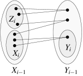
Figure 3: $X_{i}=X_{i-1}\setminus Z_{i}$ and $Y_{i}=Y_{i-1}^{X_{i}}$.

Let $1\leq i\leq k$. Since $X_{i}=X_{i-1}\setminus Z_{i}$, we have

$$e(X_{i},V\setminus Y_{i})\> =\>e(X_{i-1},V\setminus Y_{i})-e(Z_{i},V\setminus Y_{i})$$

$$\hskip-14.22636pt=\>e(X_{i-1},V\setminus Y_{i-1})+e(X_{i-1},Y_{i-1}\setminus Y_{i})-e(Z_{i},V\setminus Y_{i-1})-e(Z_{i},Y_{i-1}\setminus Y_{i})$$

$$\hskip-14.22636pt=\>e(X_{i-1},V\setminus Y_{i-1})-e(Z_{i},V\setminus Y_{i-1})+e(X_{i},Y_{i-1}\setminus Y_{i}).$$

Since $Y_{i}=Y_{i-1}^{X_{i}}$, every neighbour $u\in Y_{i-1}\setminus Y_{i}$ of a vertex in $X_{i}$ has exactly one neighbour in $Z_{i}$ (see Figure 3). Hence, $e(X_{i},Y_{i-1}\setminus Y_{i})=e(Z_{i},Y_{i-1}\setminus Y_{i-1}^{Z_{i}})$. So we have

$$e(X_{i-1},V\setminus Y_{i-1})\>=\>e(X_{i},V\setminus Y_{i})+e(Z_{i},V\setminus Y_{i-1})-e(Z_{i},Y_{i-1}\setminus Y_{i-1}^{Z_{i}}).$$

By the definition of $Z_{i}$, we have $e(Z_{i},V\setminus Y_{i-1})>e(Z_{i},Y_{i-1}\setminus Y_{i-1}^{Z_{i}})+\zeta_{S}^{*}\,|Z_{i}|$. Combining the last two expressions gives

$$e(X_{i-1},V\setminus Y_{i-1})\>>\>e(X_{i},V\setminus Y_{i})+\zeta_{S}^{*}\,|Z_{i}|.$$

Setting $Z^{*}=\bigcup\limits_{1\leq i\leq k}Z_{i}$, we have $e(X_{k},V\setminus Y_{k})<e(X_{0},V\setminus Y_{0})-\zeta_{S}^{*}\,|Z^{*}|$. As a consequence, using (2),

$$|Z^{*}|\><\>\frac{e(X_{0},V\setminus Y_{0})-e(X_{k},V\setminus Y_{k})}{\zeta_{S}^{*}}\>\leq\>\frac{e(X_{0},V\setminus Y_{0})}{\zeta_{S}^{*}}\><\>\frac{\zeta_{S}^{*}\,|X_{0}|}{\zeta_{S}^{*}}\>=\>|X_{0}|.$$

Since $X_{k}=X_{0}\setminus Z^{*}$, this implies $|X_{k}|>0$, which leads to $X_{k}\neq\varnothing$.

Finally, let $v\in X_{k}\neq\varnothing$ and assume $Y_{k}=\varnothing$. Taking $W=\{v\}$ in the inequality in (S3) (which by construction is satisfied by $(X_{k},Y_{k})$), we obtain $d(v)\leq\zeta_{S}^{*}$. Since $v$ is a big vertex, $d(v)\geq\zeta_{S}^{*}+1$. This contradiction means that we must have $Y_{k}\neq\varnothing$, which concludes the proof of Lemma 2.4.   

3.2 Proof of Lemma 2.12

We recall the hypotheses of the lemma: We have positive real numbers $\beta$ and $\zeta$; $H$ is a multigraph; each vertex $v$ of $H$ has an associated integer $\sigma(v)$; and for each edge $e$ a positive real number $b_{e}$ is given. In this subsection, all degrees $d(v)$ are in the multigraph $H$.

The following three conditions are satisfied:

(H1’)For all vertices $v$ in $H$, $d(v)\leq\sigma(v)\leq\beta$.

(H2’)For all edges $e=uv$ in $H$, $b_{e}\geq\bigl{(}\frac{3}{2}\,\beta+\frac{9}{2}\,\zeta)-(\sigma(u)-d(u))-(\sigma(v)-d(v))$.

(H3’)For all non-empty subsets $W\subseteq V(H)$, $\sum\limits_{w\,\in\,W}(\sigma(w)-d(w))\leq e_{H}(W,V(H)\setminus W)+\zeta\,|W|$.

In the proof that follows, we will show that the vector $\vec{x}=(x_{e})$, $x_{e}=1/b_{e}$, is in $\mathcal{MP}(H)$.

For an edge $e=uv$ in $H$, define

$$a_{e}\>=\>\bigl{(}\tfrac{3}{2}\,\beta+\tfrac{9}{2}\,\zeta\bigr{)}-(\sigma(u)-d(u))-(\sigma(v)-d(v))\qquad\text{and}\qquad y_{e}\>=\>\frac{1}{a_{e}}.$$ (3)

We will in fact prove that the vector $\vec{y}=(y_{e})$ is in the matching polytope $\mathcal{MP}(H)$. Since $b_{e}\geq a_{e}$, we have $x_{e}=1/b_{e}\leq 1/a_{e}=y_{e}$. So, by Edmonds’ characterisation of the matching polytope, if $\vec{y}\in\mathcal{MP}(H)$, this guarantees that $\vec{x}\in\,\mathcal{MP}(H)$, as required.

Applying condition (H3’) to the set $W=\{v\}$ gives $\sigma(v)-d(v)\leq d(v)+\zeta$, which implies:

(a)For all vertices $v\in V(H)$, we have $d(v)\geq\tfrac{1}{2}\,(\sigma(v)-\zeta)$.

Let $e=uv$ be an edge of $H$. If we use the estimate above for both $u$ and $v$ in the definition of $a_{e}$ in (3), recalling that $\sigma(u),\sigma(v)\leq\beta$, we obtain

$$a_{e}\>\geq\>\tfrac{3}{2}\,\beta+\tfrac{9}{2}\,\zeta-\tfrac{1}{2}\,\sigma(u)-\tfrac{1}{2}\,\sigma(v)-\zeta\>\geq\>\tfrac{1}{2}\beta+\tfrac{7}{2}\,\zeta.$$

On the other hand, if we use observation (a) for $u$ only, we get

$$a_{e}\>\geq\>d(v)+\tfrac{3}{2}\,\beta+\tfrac{9}{2}\,\zeta-\tfrac{1}{2}\,\sigma(u)-\sigma(v)-\tfrac{1}{2}\,\zeta\>\geq\>d(v)+4\zeta.$$

Hence, the following two conclusions hold.

(b)For all edges $e=uv$ in $E(H)$, we have $a_{e}\geq d(v)+4\zeta$.

(c)For all edges $e\in E(H)$, we have $a_{e}\geq\tfrac{1}{2}\,\beta+\tfrac{7}{2}\,\zeta$.

Note that observation (c) also gives $b_{e}\geq a_{e}\geq\tfrac{1}{2}\,\beta$ for all $e\in E(H)$, as required.

By observation (b), we find, since $\zeta>0$,

$$\sum_{e\,\ni\,v}\frac{1}{a_{e}}\>\leq\>d(v)\cdot\frac{1}{d(v)+4\zeta}\><\>1,$$

which shows that

Claim 3.4

For all vertices $v\in V(H)$, we have $\displaystyle\sum_{e\,\ni\,v}y_{e}<1$.

Using Theorem 2.10, all that remains is to prove that for all $W\subseteq V(H)$ with $|W|\geq 3$ and $|W|$ odd, we have $\sum\limits_{e\,\in\,E(W)}y_{e}\leq\tfrac{1}{2}\,(|W|-1)$. We will actually prove this for all $|W|\geq 3$. Note that we can certainly assume $E(W)\neq\varnothing$.

Using observation (b), we infer that

$$\sum_{e\,\in\,E(W)}\frac{1}{a_{e}}\>\leq\>\tfrac{1}{2}\sum_{u\,\in\,W}\frac{d_{H[W]}(u)}{d(u)+4\zeta}\>=\>\tfrac{1}{2}\sum_{u\,\in\,W}\Bigl{(}\frac{d(u)}{d(u)+4\zeta}-\frac{d(u)-d_{H[W]}(u)}{d(u)+4\zeta}\Bigr{)}.$$

Since $\dfrac{d(u)}{d(u)+4\zeta}\leq\dfrac{\beta}{\beta+4\zeta}$ and $\dfrac{d(u)-d_{H[W]}(u)}{d(u)+4\zeta}\geq\dfrac{d(u)-d_{H[W]}(u)}{\beta+4\zeta}$, this implies

$$\sum_{e\,\in\,E(W)}\frac{1}{a_{e}}\>\leq\>\tfrac{1}{2}\,|W|\,\frac{\beta}{\beta+4\zeta}-\tfrac{1}{2}\,\frac{e(W,W^{c})}{\beta+4\zeta}.$$

Here we used that $\sum\limits_{u\,\in\,W}\bigl{(}d(u)-d_{H[W]}(u)\bigr{)}=e(W,W^{c})$, where $W^{c}=V(H)\setminus W$.

If $e(W,W^{c})\geq\beta$, we obtain, since $\zeta>0$,

$$\sum_{e\,\in\,E(W)}\!y_{e}\>\leq\>\tfrac{1}{2}\,(|W|-1)\cdot\frac{\beta}{\beta+4\zeta}\><\>\tfrac{1}{2}\,(|W|-1).$$

So we can assume in the following that $e(W,W^{c})\leq\beta$, in which case Condition (H3’) of Lemma 2.12 implies

$$\sum_{u\,\in\,W}(\sigma(u)-d(u))\>\leq\>e(W,W^{c})+\zeta\,|W|\>\leq\>\beta+\zeta\,|W|.$$

For a vertex $u$ set $c(u)=\sigma(u)-d(u)$, and for a set of vertices $U$ define $c(U)=\sum\limits_{u\,\in\,U}c(u)$. So we can write the inequality above as $c(W)\leq\beta+\zeta\,|W|$.

In the following we use the fact that all $a_{e}$ are large enough to find a bound for the sum $\sum\limits_{e\,\in\,E(W)}\!a_{e}^{-1}$. To this aim, recall from (3) that $a_{e}=\bigl{(}\frac{3}{2}\,\beta+\tfrac{9}{2}\,\zeta\bigr{)}-c(u)-c(v)$ for all edges $e=uv$ in $H$. This gives

$$\sum_{e\,\in\,E(W)}\!a_{e}\>=\>\bigl{(}\tfrac{3}{2}\,\beta+\tfrac{9}{2}\,\zeta\bigr{)}\,|E(W)|-\sum_{u\,\in\,W}c(u)\,d_{H[W]}(u).$$

Since $d_{H[W]}(u)\leq d(u)=\sigma(u)-c(u)\leq\beta-c(u)$, we have

$$\sum_{e\,\in\,E(W)}\!a_{e}\>\geq\>\bigl{(}\tfrac{3}{2}\,\beta+\tfrac{9}{2}\,\zeta\bigr{)}\,|E(W)|-\beta\,c(W)+\sum_{u\,\in\,W}c(u)^{2}.$$

Set $q=\frac{3}{2}\,\beta+\tfrac{9}{2}\,\zeta$ and $p=\min\limits_{uv\in E(W)}\bigl{\{}q-c(u)-c(v)\bigr{\}}$. This means that $q-p=\max\limits_{uv\in E(W)}\bigl{\{}c(u)+c(v)\bigr{\}}$. Let $e=uv$ be an edge in $E(W)$ so that $c(u)+c(v)=q-p$. Then $c(u)^{2}+c(v)^{2}\geq\tfrac{1}{2}\,(q-p)^{2}$, and hence we can be sure that

$$\sum_{e\,\in\,E(W)}\!a_{e}\>\geq\>q\,|E(W)|-\beta\,c(W)+\tfrac{1}{2}\,(q-p)^{2}.$$

We now use this inequality and the following claim to bound $\sum\limits_{e\,\in\,E(W)}\!a_{e}^{-1}$.

Claim 3.5

Let $r_{1},\ldots,r_{m}$ be $m$ real numbers such that $0<p\leq r_{1},\dots,r_{m}\leq q$ and $\sum\limits_{1\,\leq\,i\,\leq\,m}\!r_{i}\geq q\,m-(q-p)\,S$, for some $S\geq 0$. Then we have $\sum\limits_{1\,\leq\,i\,\leq\,m}\!r_{i}^{-1}\leq\dfrac{S}{p}+\dfrac{m-S}{q}$.

• Proof  The result is trivial if $p=q$, so suppose $p<q$. For any $1\leq i\leq m$, set $c_{i}=\dfrac{q-r_{i}}{q-p}$. Now we have $0\leq c_{i}\leq 1$ for all $1\leq i\leq m$, and $\sum\limits_{1\,\leq\,i\,\leq\,m}\!c_{i}\leq S$. Since the function $x\mapsto\dfrac{1}{x}$ is convex, we have that for $1\leq i\leq m$,

  $$\frac{1}{r_{i}}\>=\>\frac{1}{q-c_{i}\,(q-p)}\>=\>\frac{1}{c_{i}\,p+(1-c_{i})\,q}\>\leq\>c_{i}\,\frac{1}{p}+(1-c_{i})\,\frac{1}{q}\>=\>c_{i}\,\Bigl{(}\frac{1}{p}-\frac{1}{q}\Bigr{)}+\frac{1}{q}.$$

  As a consequence,

  $$\sum_{1\,\leq\,i\,\leq\,m}\frac{1}{r_{i}}\>\leq\>\Bigl{(}\frac{1}{p}-\frac{1}{q}\Bigr{)}\sum_{1\,\leq\,i\,\leq\,m}c_{i}+\frac{m}{q}\>\leq\>\Bigl{(}\frac{1}{p}-\frac{1}{q}\Bigr{)}\,S+\frac{m}{q}\>\leq\>\frac{S}{p}+\frac{m-S}{q}.$$

  $\Box$

We set $R=\beta\,c(W)-\tfrac{1}{2}\,(q-p)^{2}$ and $S=\dfrac{R}{q-p}$. Using Claim 3.5, at this point we have

$$\sum_{e\,\in\,E(W)}\frac{1}{a_{e}}\>\leq\>\frac{S}{p}+\frac{|E(W)|-S}{q}\>=\>\frac{S\,(q-p)}{pq}+\frac{|E(W)|}{q}\>=\>\frac{R}{pq}+\frac{2\,|E(W)|}{3\beta+9\zeta}.$$

Notice that by condition (H3’) of Lemma 2.12, $2\,|E(W)|\leq\sum\limits_{u\,\in\,W}\sigma(u)-2c(W)+\zeta\,|W|\leq\beta\,|W|-2c(W)+\zeta\,|W|$. Hence we find

$$\sum_{e\,\in\,E(W)}\frac{1}{a_{e}}\>\leq\>\frac{\beta\,|W|}{3\beta+9\zeta}+\frac{R}{pq}-\frac{2c(W)}{3\beta+9\zeta}+\frac{\zeta\,|W|}{3\beta+9\zeta}.$$ (4)

Claim 3.6

We have $\dfrac{R}{pq}-\dfrac{2c(W)}{3\beta+9\zeta}+\dfrac{\zeta\,|W|}{3\beta+9\zeta}\leq\dfrac{\zeta}{\beta+3\zeta}\,|W|$.

• Proof   Since $q=\frac{3}{2}\,\beta+\tfrac{9}{2}\,\zeta$, we only have to prove that $\dfrac{2R}{p}-2c(W)\leq 2\zeta\,|W|$.

  Let us write $q-p=\alpha\beta$, and so $p=\tfrac{1}{2}\,(3-2\alpha)\,\beta+\tfrac{9}{2}\,\zeta$ and $R=\beta\,c(W)-\tfrac{1}{2}\,\alpha^{2}\,\beta^{2}$. We have

  $$\frac{2R}{p}-2c(W)\>=\>\frac{2\beta\,c(W)}{p}-\frac{\alpha^{2}\,\beta^{2}}{p}-2c(W).$$

  If $p\geq\beta$, this expression is negative, so we can assume that $p<\beta$. In this case, using that $c(W)\leq\beta+\zeta\,|W|$, we have

  $$\frac{2R}{p}-2c(W) \>=\>\frac{2\beta\,c(W)}{p}-\frac{\alpha^{2}\,\beta^{2}}{p}-2c(W)$$

  $$\>=\>2c(W)\,\frac{\beta-p}{p}-\frac{\alpha^{2}\,\beta^{2}}{p}\>\leq\>\frac{\beta}{p}\,(2\beta-2p-\alpha^{2}\,\beta)+2\zeta\,|W|\,\frac{\beta-p}{p}.$$

  As $2p=(3-2\alpha)\,\beta+9\zeta$, we have $2\beta-2p-\alpha^{2}\,\beta=(-1+2\alpha-\alpha^{2})\,\beta-9\zeta=-(\alpha-1)^{2}\,\beta-9\zeta<0$. Since $p=a_{e}$ for some edge $e$, we have $p\geq\tfrac{1}{2}\,\beta$ by observation (c). Hence, $(\beta-p)/p\leq 1$ and we can conclude that $2R/p-2c(W)\leq 2\zeta\,|W|$, which completes the proof of the claim.   $\Box$

Combining (4) and Claim 3.6, we obtain

$$\sum_{e\,\in\,E(W)}\!y_{e}\>=\>\sum_{e\,\in\,E(W)}\frac{1}{a_{e}}\>\leq\>\frac{\beta\,|W|}{3\beta+9\zeta}+\frac{\zeta\,|W|}{\beta+3\zeta}\>=\>\frac{\beta+3\zeta}{3\beta+9\zeta}\,|W|\>=\>\tfrac{1}{3}\,|W|.$$

Since $|W|\geq 3$, we have $\frac{1}{3}\,|W|\leq\tfrac{1}{2}\,(|W|-1)$, which completes the proof of the lemma.   

4 Proof of Theorem 1.3

We use the notation and terminology from Section 2.

We start similarly to the proof of Theorem 1.2 in Subsection 2.2. Suppose Theorem 1.3 is false. Then there exists a surface $S$ such that for any $\beta_{S},\gamma_{S}$ we can find $\beta\geq\beta_{S}$ and a graph $G$, with a $\Sigma$-system of width at most $\beta$, such that $\omega(G;\Sigma)>\tfrac{3}{2}\,\beta+\gamma_{S}$. Let $\zeta_{S}^{*}=132\,(3-\chi(S))$ be as given in Lemma 2.4. We take $\zeta_{S}=\zeta_{S}^{*}$, $\beta_{S}=\frac{2}{3}\,(\zeta_{S}^{*})^{2}=11616\,(3-\chi(S))^{2}$, and $\gamma_{S}=\tfrac{1}{2}\,\zeta_{S}^{*}+10=208-66\,\chi(S)$. Note that $\chi(S)\leq 2$, so $\beta_{S}\geq 11616$.

By assumption, there exist $\beta\geq\beta_{S}$ and a graph $G$, with a $\Sigma$-system of width at most $\beta$, containing a $\Sigma$-clique having more than $\tfrac{3}{2}\,\beta+\gamma_{S}$ vertices. Choose such graph $G$ with the minimum number of vertices, and, with respect to that, with the maximum number of edges.

Similarly as in the proof of Theorem 1.2, we can assume $G$ is connected, has at least 17424 vertices, and is edge-maximal with respect to being embeddable in $S$. By Lemma 2.3 we get that each vertex has degree at least three.

The following is an easy observation.

Claim 4.1

For any vertex $v$, every $\Sigma$-clique containing $v$ has size at most $1+d^{\Sigma}(v)$.

Next we prove the following.

Claim 4.2

Let adjacent vertices $v,u$ satisfy $d(v)\leq 5$ and $d(u)\leq\zeta_{S}$. Then $v$ is in every $\Sigma$-clique of size larger than $\frac{3}{2}\,\beta+\gamma_{S}$, and $d^{\Sigma}(v)\geq\frac{3}{2}\,\beta+\gamma_{S}$.

• Proof   The argument is similar to the one in Subsection 2.2.2: Construct a graph $G_{2}$ by contracting the edge $vu$ into a new vertex $w$ (remove multiple edges if they appear). Set $V_{2}=(V\setminus\{v,u\})\cup\{w\}$. Let $\Sigma_{2}(w)=\Sigma(u)\cup\Sigma(v)\setminus\{u,v\}$. For a vertex $t\in V_{2}\setminus\{w\}$, if $\Sigma(t)$ contains $u$, then set $\Sigma_{2}(t)=(\Sigma(t)\setminus\{u,v\})\cup\{w\}$; otherwise, set $\Sigma_{2}(t)=\Sigma(t)\setminus\{v\}$. Note that $G_{2}$ is smaller than $G$ and is still embeddable in $S$. Moreover, for every $t\in V_{2}\setminus\{w\}$, we have $|\Sigma_{2}(t)|\leq|\Sigma(t)|\leq\beta$; while for $w$ we have $|\Sigma_{2}(w)|\leq|\Sigma(u)|+|\Sigma(v)|\leq d_{G}(u)+d_{G}(v)\leq 5+\zeta_{S}\leq\beta$.

  By construction, it is easy to check that every $\Sigma$-clique in $G$ not containing $v$ corresponds to a $\Sigma_{2}$-clique in $G_{2}$ of the same size. Since $G$ was chosen as a smallest counterexample, this means that every $\Sigma$-clique in $G$ of size larger than $\frac{3}{2}\,\beta+\gamma_{S}$ must contain $v$.

  For the second part we use that $G$, as a counterexample, must contain $\Sigma$-cliques larger than $\frac{3}{2}\,\beta+\gamma_{S}$, whereas any $\Sigma$-clique in $G$ containing $v$ has size at most $1+d^{\Sigma}(v)$.   $\Box$

We continue going through the cases of Lemma 2.4. If all vertices of $G$ have degree at most $\zeta_{S}$, then the number of $\Sigma$-neighbours of any vertex is at most $(\zeta_{S})^{2}$. So the maximum size of a $\Sigma$-clique is at most $(\zeta_{S})^{2}+1\leq\frac{3}{2}\,\beta+1\leq\frac{3}{2}\,\beta+\gamma_{S}$, a contradiction.

Next suppose there is a vertex $v$ of degree at most five with at most one neighbour of degree more than $\zeta_{S}$. Then, since $\beta\geq\tfrac{2}{3}\,(\zeta_{S}^{*})^{2}\geq 8\zeta_{S}^{*}$, we have

$$d^{\Sigma}(v)\>\leq\>d(v)+\!\!\!\sum_{t\,\in\,N(v),\;v\,\in\,\Sigma(t)}\!\!\!(|\Sigma(t)|-1)\>\leq\>5+4\,(\zeta_{S}^{*}-1)+(\beta-1)\>=\>4\zeta_{S}^{*}+\beta\>\leq\>\tfrac{3}{2}\,\beta.$$

But every vertex has degree at least three, hence $v$ has a neighbour $u$ of degree at most $\zeta_{S}^{*}$. We obtain a contradiction with Claim 4.2.

Let $X$ and $Y$ be the two disjoint, non-empty, sets forming a very special $\zeta_{S}^{*}$-pair in $G$ satisfying (S3) in Lemma 2.4. For convenience, we repeat the essential properties of those sets:

(i)Every vertex in $X$ has degree at least $\zeta_{S}^{*}+1$. Every vertex $y\in Y$ has degree four, is adjacent to exactly two vertices of $X$, and the remaining neighbours of $y$ have degree four as well.

(ii)For all pairs of vertices $y,z\in Y$, if $y$ and $z$ are adjacent or have a common neighbour $w\notin X$, then $X^{y}=X^{z}$.

(iii)For all non-empty subsets $W\subseteq X$, we have $e(W,V\setminus Y)\leq e(W,Y\setminus Y^{W})+\zeta_{S}^{*}\,|W|$.

We can remove from $X$ any vertex not adjacent to any vertex in $Y$.

We can use arguments similar to the first part of Subsection 2.2.3 to show the following.

Claim 4.3

For all $y\in Y$, we have that if $X^{y}=\{x_{1},x_{2}\}$, then $y\in\Sigma(x_{1})\cap\Sigma(x_{2})$.

Next, by (i), every $y\in Y$ has degree four and a neighbour $u$ of degree four. From Claim 4.2 we can conclude:

Claim 4.4

For every $y\in Y$, we have that $y$ is in every $\Sigma$-clique of size larger than $\frac{3}{2}\,\beta+\gamma_{S}$, and $d^{\Sigma}(y)\geq\frac{3}{2}\,\beta+\gamma_{S}$.

Also by the properties of the vertices in $Y$ according to (i) and (ii), we have for all $y\in Y$ and $X^{y}=\{x_{1},x_{2}\}$,

$$d^{\Sigma}(y)\> \leq\>4+2\cdot(4-1)+|\Sigma(x_{1})\setminus\{y\}|+|\Sigma(x_{2})\setminus\{y\}|-|Y^{\{x_{1},x_{2}\}}\setminus\{y\}|$$

$$=\>9+|\Sigma(x_{1})|+|\Sigma(x_{2})|-|Y^{\{x_{1},x_{2}\}}|$$

Here we use that by Claim 4.3 all vertices in $Y^{\{x_{1},x_{2}\}}$ are contained in both $\Sigma(x_{1})$ and $\Sigma(x_{2})$; hence we can subtract the term $|Y^{\{x_{1},x_{2}\}}\setminus\{y\}|$, since these vertices are counted twice in $|\Sigma(x_{1})\setminus\{y\}|+|\Sigma(x_{2})\setminus\{y\}|$. Since $|\Sigma(x_{1})|,|\Sigma(x_{2})|\leq\beta$, from Claim 4.4 we can conclude the following.

Claim 4.5

For every pair $x_{1},x_{2}\in X$ for which there is a $y\in Y$ with $X^{y}=\{x_{1},x_{2}\}$, we have $|Y^{\{x_{1},x_{2}\}}|\leq\tfrac{1}{2}\,\beta-\gamma_{S}+9$.

Since every vertex in $Y$ is in every $\Sigma$-clique of size larger than $\frac{3}{2}\,\beta+\gamma_{S}$, and by the hypothesis there is at least one such clique, we must have that all pairs of vertices in $Y$ are adjacent or appear together in some $\Sigma(v)$. By (ii), this proves that for every two vertices $y_{1},y_{2}\in Y$, we have $X^{y_{1}}\cap X^{y_{2}}\neq\varnothing$. As a consequence, if $G_{X}$ denotes the graph with vertex set $X$ in which two vertices are adjacent if they have a common neighbour in $Y$, then $G_{X}$ is either a triangle or a star. (Here we use that we can assume all vertices in $X$ to have at least one neighbour in $Y$.)

Case 1. $G_{X}$ is a triangle.
Let $X=\{x_{1},x_{2},x_{3}\}$. This means that $Y=Y^{\{x_{1},x_{2}\}}\cup Y^{\{x_{1},x_{3}\}}\cup Y^{\{x_{2},x_{3}\}}$, and so by Claim 4.5 we get $|Y|\leq\frac{3}{2}\,\beta-3\gamma_{S}+27$.

Since $Y^{X}=Y$ by definition of $X$, we have $e(X,Y\setminus Y^{X})=0$. So using the inequality in (iii) with $W=X$ leads to $e(X,V\setminus Y)\leq 3\zeta_{S}^{*}$. That means there must be $x_{j_{1}}$ and $x_{j_{2}}$ such that $e(\{x_{j_{1}},x_{j_{2}}\},V\setminus Y)\leq 2\zeta_{S}^{*}$. And so for $y\in Y^{\{x_{j_{1}},x_{j_{2}}\}}$, we can estimate, using (i) and $|X|=3$,

$$d^{\Sigma}(y)\> \leq\>2+2\cdot(4-1)+|X|+(|Y|-1)+e(\{x_{j_{1}},x_{j_{2}}\},V\setminus(X\cup Y))$$

$$\leq\>\tfrac{3}{2}\,\beta-3\gamma_{S}+37+2\zeta_{S}^{*}.$$

But this contradicts Claim 4.4, since $4\gamma_{S}>2\zeta_{S}^{*}+37$.

Case 2. $G_{X}$ is a star.
We denote by $x$ the vertex of $X$ corresponding to the centre of the star $G_{X}$, and by $x_{1},\ldots,x_{k}$, $k\geq 1$, the vertices of $X$ corresponding to the leaves.

Using the inequality in (iii) with $W=X$ again, we get $e(X,V\setminus Y)\leq\zeta_{S}^{*}\,|X|=(k+1)\,\zeta_{S}^{*}$. Since $X=\{x,x_{1},\ldots,x_{k}\}$, there must be an $x_{j}$ such that $e(\{x_{j}\},V\setminus Y)\leq\dfrac{1}{k}\,(k+1)\,\zeta_{S}^{*}\leq 2\zeta_{S}^{*}$. Now for $y\in Y^{\{x,x_{j}\}}$, we can estimate

$$d^{\Sigma}(y)\>\leq\>4+2\cdot(4-1)+|(\Sigma(x)\cup\Sigma(x_{j}))\setminus\{y\}|\>=\>9+|\Sigma(x)|+|\Sigma(x_{j})\setminus\Sigma(x)|.$$

Since $Y\subseteq\Sigma(x)$, we have $|\Sigma(x_{j})\setminus\Sigma(x)|\leq e(\{x_{j}\},V\setminus Y)\leq 2\zeta_{S}^{*}$. Together with $|\Sigma(x)|\leq\beta$, this means $d^{\Sigma}(y)\leq\beta+9+2\zeta_{S}^{*}$. This contradicts Claim 4.4, since $\tfrac{1}{2}\,\beta>9+2\zeta_{S}^{*}$.   

In the proof of Theorem 1.3, we used $\beta_{S}=11616\,(3-\chi(S))^{2}$ and $\gamma_{S}=208-66\,\chi(S)$. Since the sphere $\mathbb{S}^{2}$ has $\chi(\mathbb{S}^{2})=2$, following the proof above means we can obtain $\beta_{P}=11616$ and $\gamma_{P}=76$ for the planar case. But it is clear that these values are far from best possible. Using more careful estimates in the proof above and more careful reasoning in certain parts of the proof of Lemma 2.4 can give significantly smaller values. Since our first goal is to show that we can obtain constant values for these results, we do not pursue this further.

5 Concluding Remarks and Discussion

5.1 About the Proof

The proof of our main theorem for major parts follows the same lines as the proof of Theorem 1.6 in [10]. In particular, the proof of that theorem also starts with a structural lemma comparable to Lemma 2.4, uses the structure of the graph to reduce the problem to edge-colouring a specific multigraph, and then applies (and extends) Kahn’s approach to that multigraph. Of course, a difference is that Theorem 1.6 only deals with list colouring the square of a graph, but it is probably possible to generalise the whole proof to the case of list $\Sigma$-colouring. Nevertheless, there are some important differences in the proofs we feel deserve highlighting.

Lemma 2.4 is stronger than the comparable [10, Lemma 3.3]. We obtain a set $Y$ of vertices with degree four and with a very specific structure of their neighbourhoods. This structure allows us to construct a multigraph $H$ so that a standard list edge-colouring of $H$ provides the information to colour the vertices in $Y$ (see Lemma 2.7). In the lemma in [10], the vertices in the comparable set $Y$ are only guaranteed to have degree at most $\Delta^{1/4}$, and knowledge about their neighbourhood is far sketchier. This means that the translation to list edge-colouring of a multigraph is not so clean; apart from the normal condition in the list edge-colouring of $H$ (that adjacent edges need different colours), for each edge there may be up to $O(\Delta^{1/2})$ non-adjacent edges that also need to get a different colour. In particular this means that in [10], Kahn’s result in Theorem 2.11 cannot be used directly. Instead, a new, stronger, version has to be proved that can deal with a certain number of non-adjacent edges that need to be coloured differently. Lemma 2.4 allows us to use Kahn’s Theorem directly.

A second aspect in which our Lemma 2.4 is stronger is that in the final condition (S3), we have an ‘error term’ that is a constant times $|W|$. In [10] the comparable term is $\Delta^{9/10}\,|W|$, where $\Delta$ is the maximum degree of the graph. This in itself already means that the approach in [10] at best can give a bound of the type $\frac{3}{2}\,\Delta+o(\Delta)$. The fact that we cannot do better with the stronger structural result is because of the limitations of Kahn’s Theorem, Theorem 2.11. If it would be possible to replace the condition in that theorem by a condition of the form ‘the vector $\vec{x}=(x_{e})$ with $x_{e}=\tfrac{1}{|L(e)|-K}$ for all $e\in E(H)$ is an element of $\mathcal{MP}(H)$’, where $K$ is some positive constant, the work in this paper would directly give an improvement for the bound in Theorem 1.2 to $\frac{3}{2}\,\beta+O(1)$. Note that our version of Lemma 2.12 is also already strong enough to support that case.

Lemma 2.4 also allows us to prove a bound $\frac{3}{2}\,\beta+O(1)$ for the $\Sigma$-clique number in Theorem 1.3. The important corollary that the square of a graph embeddable in a fixed surface has clique number at most $\frac{3}{2}\,\Delta+O(1)$ would have been impossible without the improved bound in the lemma.

Also Lemma 2.12 is stronger than its compatriot [10, Lemma 5.9]. The lemma in [10] only deals with the case $d_{G}(v)=\beta$ for all vertices $v$ in $H$. Because of this, it can only be applied to the case that all vertices in $H$ have maximum degree $\Delta(G)$ in $G$. Some non-trivial trickery then has to be used to deal with the case that there are vertices in $H$ of degree less than $\Delta(G)$ in $G$. Moreover, the proof of Lemma 2.12 is completely different from the proof in [10]. We feel that our new proof is more natural and intuitive, giving a clear relation between the lower bounds on the sizes of the lists and the upper bound of the sum of their inverses. The proof in [10] is more ad-hoc, using some non-obvious distinction in a number of different cases, depending on the size of $W$ and the degrees of some vertices in $W$.

5.2 Further Work

We feel that our work is just the beginning of the study of general $\Sigma$-colouring problems. It should be possible to obtain deeper results taking into account the structure of the $\Sigma$-system, and not just the sizes of the sets $\Sigma(v)$. The following easy result is an example of this.

Recall that a graph is $q$-degenerate if there exists an ordering $v_{1},v_{2},\dots,v_{n}$ of the vertices such that every $v_{i}$ has at most $q$ neighbours in $\{v_{1},\dots,v_{i-1}\}$. A class of graphs is degenerate if there is some $q$ such that every graph in the class is $q$-degenerate. Examples of degenerate graph classes are graphs embeddable in a fixed surface, and proper minor-closed classes.

Proposition 5.1

For any degenerate graph class $\mathcal{F}$, there exists a constant $c_{\mathcal{F}}$ such that the following holds. Let $G$ be a graph in $\mathcal{F}$, together with a $\Sigma$-system so that $\Sigma(u)\cap\Sigma(v)=\varnothing$ for every two distinct vertices $u,v$. Then $\mathit{ch}(G;\Sigma)\leq\Delta(G;\Sigma)+c_{\mathcal{F}}$.

• Proof  Suppose every graph in $\mathcal{F}$ is $q$-degenerate, and set $c_{\mathcal{F}}=q+1$. For a graph $G$ in $\mathcal{F}$, take an ordering $v_{1},\ldots,v_{n}$ of its vertices such that each $v_{i}$ has at most $q$ neighbours in $\{v_{1},\ldots,v_{i-1}\}$. We greedily colour the vertices $v_{1},\ldots,v_{n}$ in $G$ in that order.

  Note that by the hypothesis, each vertex $v$ has at most one neighbour $w$ with $v\in\Sigma(w)$. When colouring the vertex $v_{i}$, we need to take into account its neighbours in $\{v_{1},\ldots,v_{i-1}\}$, plus the vertices in $\Sigma(w)\cap\{v_{1},\ldots,v_{i-1}\}$ for a vertex $w$ with $v_{i}\in\Sigma(w)$ (where that vertex $w$ can be in $\{v_{i+1},\ldots,v_{n}\}$). By construction of the ordering, there are at most $q$ neighbours of $v_{i}$ in $\{v_{1},\ldots,v_{i-1}\}$. And a vertex $w$ with $v_{i}\in\Sigma(w)$ has at most $|\Sigma(w)|\leq\Delta(G;\Sigma)$ vertices in $\Sigma(w)\cap\{v_{1},\ldots,v_{i-1}\}$. So the total number of forbidden colours when colouring $v_{i}$ is at most $\Delta(G;\Sigma)+q$. Since each vertex has $\Delta(G;\Sigma)+q+1$ colours available, the greedy algorithm will always find a free colour.   

We think that it is possible to combine our main theorem and the theorem above in the following way. For a $\Sigma$-system for a graph $G$, let $k(G;\Sigma)$ be the maximum of $|\Sigma(u)\cap\Sigma(v)|$ over all pairs $u,v$ of distinct vertices.

Conjecture 5.2

Let $S$ be a fixed surface. Then there exists a constant $c_{S}$ such that for all graphs $G$ embeddable in $S$, with a $\Sigma$-system, we have

$$\mathit{ch}(G;\Sigma)\>\leq\>\Delta(G;\Sigma)+k(G;\Sigma)+c_{S}.$$

This conjecture would fit with our current proof of Theorem 1.2, the main part of which is a reduction of the original problem to a list edge-colouring problem. For this approach, Shannon’s Theorem [31] that a multigraph with maximum degree $\Delta$ has an edge-colouring using at most $\bigl{\lfloor}\frac{3}{2}\,\Delta(G)\bigr{\rfloor}$ colours, forms a natural base for the bounds conjectured in Conjecture 1.1. If the relation between colouring the square of graphs embeddable in a fixed surface and edge-colouring multigraphs holds in a stronger sense, then Conjecture 5.2 forms a logical extension of Vizing’s Theorem [32] that a multigraph with maximum degree $\Delta$ and maximum edge-multiplicity $\mu$ has an edge-colouring with at most $\Delta+\mu$ colours.

In Borodin et al. [5], a weaker version of Conjecture 5.2 for cyclic colouring of plane graphs was proved. Recall that if $G^{P}$ is a plane graph, then $\Delta^{*}$ is the maximum number of vertices in a face. Let $k^{*}$ denote the maximum number of vertices that two faces of $G^{P}$ have in common.

Theorem 5.3 (Borodin, Broersma, Glebov & Van den Heuvel [5])

For a plane graph $G^{P}$ with $\Delta^{*}\geq 4$ and $k^{*}\geq 4$, we have $\chi^{*}(G^{P})\leq\Delta^{*}+3k^{*}+2$.

$\Sigma$-Colouring and Minor-Closed Classes.

It seems natural to expect that our work on graphs embeddable in a fixed surface can be extended to arbitrary proper minor-closed classes of graphs. Compare our main Theorem 1.2 with Theorem 1.6, the main result from [10]. But there exist some obstacles to a direct generalisation.

It is easy to show that if a graph $G$ is $q$-degenerate, then its square is $((2q-1)\,\Delta(G))$-degenerate. It is well-known, see e.g. [22], that for every proper minor-closed family $\mathcal{F}$, there is a constant $C_{\mathcal{F}}$ such that every graph in $\mathcal{F}$ is $C_{\mathcal{F}}$-degenerate. Hence $G^{2}$ is $((2C_{\mathcal{F}}-1)\,\Delta(G))$-degenerate, and so for every $G\in\mathcal{F}$, we have $\mathit{ch}(G^{2})\leq(2C_{\mathcal{F}}-1)\,\Delta(G)+1$.

For $\Sigma$-colouring, there is no comparable upper bound on $\mathit{ch}(G;\Sigma)$ in terms of the degeneracy of $G$ and $\Delta(G;\Sigma)$. To see this, let $G$ be the graph obtained from the complete graph $K_{n}$, $n\geq 4$, by subdividing all edges of $K_{n}$ once. For a vertex $v$ corresponding to an original vertex in $K_{n}$, set $\Sigma(v)=\varnothing$; while for a “new” vertex $v$ of degree two, set $\Sigma(v)=N_{G}(v)$. Then we have that $G$ is 2-degenerate and $\Delta(G;\Sigma)=2$, but $\mathit{ch}(G;\Sigma)=n$.

Nevertheless, combining the Robertson and Seymour graph minor structure theorem [28] with our main theorem on graphs embeddable in bounded genus surfaces, one can fairly easily obtain the following.

Theorem 5.4

Let $\mathcal{F}$ be a proper minor-closed family of graphs. Then there exist constants $C_{\mathcal{F}}$ and $c_{\mathcal{F}}$ such that the following holds: For any graph $G$ in $\mathcal{F}$ with a $\Sigma$-system, we have $\mathit{ch}(G;\Sigma)\leq C_{\mathcal{F}}\,\Delta(G;\Sigma)+c_{\mathcal{F}}$.

Giving more details of the ideas of the proof would require a number of additional definitions, and is beyond the scope of this short discussion. It would be interesting to find a proof of this theorem that does not require the full force of the graph minor structure theorem.

Also finding the smallest possible constant $C_{\mathcal{F}}$ for certain minor-closed families $\mathcal{F}$ appears an interesting question. Theorem 1.6 clearly suggests that if $\mathcal{F}_{k}$ denotes the class of $K_{3,k}$-minor free graphs ($k\geq 3$), $C_{\mathcal{F}_{k}}$ should be equal to $3/2$.

6 Kahn’s Work on List Edge-Colourings

As mentioned earlier, Theorem 2.11 is not explicitly stated in [17], but is implicit in the proof of the main result of that paper. In this final section, we give an overview of how this theorem can be obtained from the ideas in Kahn’s paper.

The main result in [17] is that the list chromatic index is asymptotically equal to the fractional chromatic index of a multigraph.

Theorem 6.1 (Kahn [17])

For any $\varepsilon>0$, there exists a $\Delta_{\varepsilon}$ such that for all $\Delta\geq\Delta_{\varepsilon}$ the following holds. If $H$ is a multigraph with maximum degree at most $\Delta$, then

$$\chi^{\prime}_{f}(H)\>\leq\>\chi^{\prime}(H)\>\leq\>\mathit{ch}^{\prime}(H)\>\leq\>(1+\varepsilon)\,\chi^{\prime}_{f}(H).$$

Here $\chi^{\prime}(H)$ is the normal chromatic index (or edge-chromatic number) of $H$, $\chi^{\prime}_{f}(H)$ is the fractional chromatic index of $H$, and $\mathit{ch}^{\prime}(H)$ is the list chromatic index of $H$. The crucial step to relate this result to the matching polytope $\mathcal{MP}(H)$ is the following well-known characterisation of the fractional chromatic index:

$$\chi^{\prime}_{f}(H)\>=\>\min\{\,\gamma>0\mid\text{the vector $(x_{e})_{e\in E(H)}$ with $x_{e}=\gamma^{-1}$ is in $\mathcal{MP}(H)$}\,\}.$$

So Theorem 6.1 is just a special case of Theorem 2.11 if we set $|L(e)|\geq\dfrac{\chi^{\prime}_{f}(H)}{1-\delta}$ for all edges $e$. (The second condition of Theorem 2.11 is automatically satisfied in that case, since trivially $\chi^{\prime}_{f}(H)\geq\Delta(H)$.)

In order to prove Theorem 6.1, Kahn describes a randomised iterative procedure that colours the edges of $H$ in a number of stages. During this procedure, the lists of available colours for each edge will change, and the lists will not be the same size for the uncoloured edges. This is why, roughly speaking, Kahn’s actual proof deals with the more general case, as described in Theorem 2.11.

In order to give the reader a better understanding of the background of Kahn’s approach, we give an overview of the crucial elements in the following subsections.

6.1 Hardcore Distributions

Hardcore distributions are distributions that originally arose in Statistical Physics, and that satisfy very natural conditions which generally provide strong independence properties allowing good sampling from a given family. Given a family of subsets $\mathcal{F}$ of a given set $\mathcal{E}$, a natural way of picking at random an element of $\mathcal{F}$ (or, in an other words, a probability distribution on $\mathcal{F}$) is as follows.

Let us suppose that each element $e$ of $\mathcal{E}$ has been assigned a positive weight $\lambda_{e}$. Then we pick each element $M\in\mathcal{F}$ with probability proportional to $\prod\limits_{e\,\in\,M}\lambda_{e}$. More precisely, the probability $P_{M}$ of picking $M\in\mathcal{F}$ at random is given by

$$P_{M}\>=\>\frac{\prod\limits_{e\,\in\,M}\lambda_{e}}{\sum\limits_{M^{\prime}\,\in\,\mathcal{F}}\>\prod\limits_{e\,\in\,M^{\prime}}\lambda_{e}}.$$

We define the vector $\vec{x}=(x_{e})_{e\in\mathcal{E}}$ by setting $x_{e}=\sum\limits_{M\,\in\,\mathcal{F},\;e\in M}\!\!P_{M}$. It is clear that $x_{e}$ is the probability that a given random element of $\mathcal{F}$ contains the element $e$. The probability distribution $\{P_{M}\}$ is called a hardcore distribution with activities $\{\lambda_{e}\}$ and marginals $\{x_{e}\}$. The vector $\vec{x}$ is called the marginal vector associated with the hardcore distribution $\{P_{M}\}$.

Given a vector $\vec{x}$, it is not always true that $\vec{x}$ is the marginal vector of some hardcore distribution. Indeed if $\mathcal{P}(\mathcal{F})$ denotes the polytope defined by taking the convex hull of the characteristic vectors of the elements of $\mathcal{F}$ , then the marginal vector $\vec{x}$ of a hardcore distribution is in $\mathcal{P}(\mathcal{F})$:

$$\vec{x}\>=\>\sum_{M\,\in\,\mathcal{F}}P_{M}\,\textbf{1}_{M}.$$

This provides a necessary condition for a vector to be the marginal vector of a hardcore distribution. It is not difficult to prove that the activities $\lambda_{e}$ corresponding to $\vec{x}$, if they exist, are unique.

From now on, let $H$ be a given multigraph. We recall that $\mathcal{M}(H)$ and $\mathcal{MP}(H)$ are the family of matchings and the matching polytope of $H$, respectively. (So $\mathcal{M}(H)$ will play the role of the family $\mathcal{F}$ from above. And using the notation from above means $\mathcal{MP}(H)=\mathcal{P}(\mathcal{M}(H))$.)

We have the following theorem relating the matching polytope and hardcore distributions.

Theorem 6.2 (Lee [20], Rabinovich et al. [27])

For a given real number $0<\delta<1$, suppose $\vec{x}$ is a vector in $(1-\delta)\,\mathcal{MP}(H)$, for some multigraph $H$. Then there exists a unique family of activities $\lambda_{e}$ such that $\vec{x}$ is the marginal vector of the hardcore distribution on the matchings of $H$ defined by the $\lambda$’s. The hardcore distribution $\{P_{M}\}_{M\in\mathcal{M}(H)}$ is the unique distribution maximising the entropy function

$$\mathcal{H}({Q_{M}})\>=\>-\!\sum_{M\,\in\,\mathcal{M}(H)}\!Q_{M}\,\log(Q_{M})$$

among all the distributions $\{Q_{M}\}_{M\in\mathcal{M}(H)}$ satisfying $\vec{x}=\!\sum\limits_{M\,\in\,\mathcal{M}(H)}\!Q_{M}\,\textbf{1}_{M}$.

Kahn and Kayll proved in [18] a family of results, resulting in a long-range independence property for the hardcore distributions defined by a marginal vector $\vec{x}$ inside $(1-\delta)\,\mathcal{MP}(H)$, see [17]. We refer to the original papers of Kahn [16, 17] and Kahn and Kayll [18], and the book by Molloy and Reed [24] for more on these issues. We settle here for citing the following lemma.

Lemma 6.3 ([18, Lemma 4.1])

For every $\delta$, $0<\delta<1$, there is a $\rho_{\delta}>0$ such that if $\{P_{M}\}$ is a hardcore distribution on the matchings of $H$ with marginal vector $\vec{x}\in(1-\delta)\,\mathcal{MP}(H)$, then for all $u,v\in V(H)$,

$$\mathbf{Pr}(\text{$M$ does not touch $u$ and $v$})\>>\>\rho_{\delta}.$$

6.2 Hardcore Distributions and Edge-Colouring

We present here Kahn’s algorithm for list edge-colouring of multigraphs first introduced and analysed in [17]. We continue to use the notation of the previous subsection. In particular, we suppose that $H$ is a multigraph and $L$ a list assignment of colours to the edges of $H$ so that the conditions of Theorem 2.11 are satisfied. By Lemma 6.2 there exists a hardcore distribution $\{P_{M}\}$ with marginals $\{|L(e)|^{-1}\}_{e\in E(H)}$, which in addition satisfies the property of Lemma 6.3. Let $\{\lambda_{e}\}$ be the activities on the edges (which are unique by Theorem 6.2) corresponding to this distribution. An extra property is indeed true: For every subgraph $H^{*}$ of $H$ it is possible to find a hardcore distribution $\{P^{*}_{M}\}$ with corresponding marginals $|L(e)|^{-1}$ for $e\in E(H^{*})$. The corresponding activities $\lambda^{*}_{e}$ will in general be different from the $\lambda_{e}$’s.

The algorithm works as follows: Let $\mathcal{L}=\!\bigcup\limits_{e\in E(H)}\!L(e)$ be the union of the colours in the lists. For each colour $\alpha$, let us define the colour graph $H_{\alpha}$ to be the graph containing all the edges whose lists contain the colour $\alpha$. And denote by $\{\lambda_{\alpha,e}\}$ the activities producing the hardcore distribution with marginals $|L(e)|^{-1}$ for $e\in E(H_{\alpha})$. The colouring procedure consists in a finite number of iterations of a procedure that we may call naive colouring. At step $i$ of the iteration, we are left with subgraphs $H^{i}_{\alpha}$ containing some uncoloured edges whose lists contain the colour $\alpha$. Of course we have $H^{i}_{\alpha}\subseteq H^{i-1}_{\alpha}\subseteq\dots\subseteq H^{0}_{\alpha}=H_{\alpha}.$

The naive colouring procedure at step $i+1$ consists of the following sub-steps.

(a)For each colour $\alpha\in\mathcal{L}$, choose independently of the other colours a random matching $M^{i+1}_{\alpha}\subseteq E(H^{i}_{\alpha})$ according to the hardcore distribution defined by the activities $\lambda_{\alpha,e}$ on the edges $e\in E(H^{i}_{\alpha})$.

(b)If an edge $e$ is in one or more of the matchings $M^{i+1}_{\alpha}$ chosen above, then choose one of the colours from those, chosen uniformly at random, and colour $e$ with that colour.

(c)For each colour $\alpha$, form $H^{i+1}_{\alpha}$ by removing from $H^{i}_{\alpha}$ all the edges that received some colour at this stage, and all vertices that are incident to one of the edges coloured with $\alpha$. (While removing a vertex, all the edges incident to it are of course removed as well.)

Note that the process above can be described also in terms of subgraphs $H^{i}$ of the original multigraph $H$, where the edges of $H^{i}$ are the edges that are still uncoloured after step $i$, and each edge $e$ in $H^{i}$ has a list of colours $L^{i}(e)$ formed by all colours $\alpha$ for which $e\in E(H^{i}_{\alpha})$. Also note that the activities $\lambda_{\alpha,e}$ remain unchanged all through the process.

A sufficient number of iterations of the naive colouring procedure results in a graph $H^{I}$, consisting of all the uncoloured edges at this step, such that $H^{I}$ has maximum degree $T$, for some integer $T$, and that the list sizes are at least $2T$, i.e., each uncoloured edge is in at least $2T$ of the $H^{I}_{\alpha}$’s. (Remember that the conditions of Theorem 2.11 imply that the lists are quite large at the beginning.) At this stage it is easy to finish the procedure by a simple greedy algorithm.

The heart of the analysis of the above algorithm in Kahn’s approach is the following strong lemma, the proof of which can be found in [17]. (To avoid confusion between an edge ‘$e$’ and the base of the natural logarithms 2.718…, we will use a roman ‘$\mathrm{e}$’ for the latter one.)

Lemma 6.4 (Kahn [17, Lemma 3.1] )

For each $K>0$ and $0<\eta<1$, there are constants $0<\xi_{K,\eta}\leq\eta$ and $\Delta_{K,\eta}$ such that the following holds for all $\Delta\geq\Delta_{K,\eta}$. Let $H$ be a multigraph with lists $L(e)$ of colours for each edge $e$. For each colour $\alpha$, define the colour graph $H_{\alpha}$ as above. Finally, for each colour $\alpha$ we are given a hardcore distribution on the matchings of $H_{\alpha}$ with activities $\{\lambda_{\alpha,e}\}_{e\in E(H_{\alpha})}$ and marginals $\{x_{\alpha,e}\}_{e\in E(H_{\alpha})}$. Suppose the following conditions are satisfied:

$\bullet$for every vertex $v$, $d_{H}(v)\leq\Delta$;

$\bullet$for every colour $\alpha$ and edge $e\in E(H_{\alpha})$, $\lambda_{\alpha,e}\leq\dfrac{K}{\Delta}$; and

$\bullet$for every edge $e$, $1-\xi_{K,\eta}\leq\sum\limits_{\alpha\,in\,L(e)}\!x_{\alpha,e}\leq 1+\xi_{K,\eta}$.

Then with positive probability the naive colouring procedure described above gives matchings $M_{\alpha}\subseteq E(H_{\alpha})$ for all colours $\alpha$, so that if we set $H^{*}=H-\bigcup_{\alpha^{\prime}}M_{\alpha^{\prime}}$, $H^{*}_{\alpha}=H_{\alpha}-V(M_{\alpha})-\bigcup_{\alpha^{\prime}}M_{\alpha^{\prime}}$, and form lists $L^{*}(e)$ for all edges $e\in E(H^{*})$ by removing no longer allowed colours from $L(e)$, we have:

$\bullet$for every vertex $v$, $d_{H^{*}}(v)\leq\dfrac{1+\eta}{1+\xi_{K,\eta}}\,\mathrm{e}^{-1}\,\Delta$; and

$\bullet$for every edge $e$ in $H^{*}$, $1-\eta\leq\sum\limits_{\alpha\,\in\,L^{*}(e)}\!x^{*}_{\alpha,e}\leq 1+\eta$.

Here $\{x^{*}_{\alpha,e}\}_{e\in E(H^{*}_{\alpha})}$ are the marginals associated to $\lambda_{\alpha,e}$ in $H^{*}_{\alpha}$.

In other words, the lemma guarantees that after one iteration of the naive colouring procedure, with positive probability the multigraph formed by the uncoloured edges has maximum degrees bounded by $\dfrac{1+\eta}{1+\xi_{K,\eta}}\,\mathrm{e}^{-1}\,\Delta$, while the sum of the marginal probabilities $x^{*}_{\alpha,e}$ for every edge $e$ will be close to 1.

In the next subsection we will combine all the strands and use the lemma above to conclude the proof of Theorem 2.11.

6.3 Completing the Proof of Theorem 2.11 — after Kahn

Let $0<\delta<1$ and $\nu>0$. We must prove the existence of a $\Delta_{\delta,\nu}$ such that for $\Delta\geq\Delta_{\delta,\nu}$ the following holds. Let $H$ be a multigraph and $L$ a list assignment of colours to the edges of $H$ so that

$\bullet$for every vertex $v$, $d_{H}(v)\leq\Delta$;

$\bullet$for all edges $e\in E(H$), $|L(e)|\geq\nu\,\Delta$;

$\bullet$the vector $\vec{x}=(x_{e})$ with $x_{e}=\dfrac{1}{|L(e)|}$ for all $e\in E(H)$ is an element of $(1-\delta)\,\mathcal{MP}(H)$.

Then there should exist a proper edge-colouring of $H$, where each edge receives a colour from its own list.

For each colour $\alpha$, define the colour graph $H_{\alpha}$ as in the previous subsection. For each colour $\alpha$ and edge $e$, set $x_{\alpha,e}=x_{e}=\dfrac{1}{|L(e)|}$, and let $\{\lambda_{\alpha,e}\}_{e\in E(H_{\alpha})}$ be the activities associated with the marginals $x_{\alpha,e}$ on $H_{\alpha}$.

Since for every edge $e$ we have $\sum\limits_{\alpha\,\in\,L(e)}\!x_{\alpha,e}=\sum\limits_{\alpha\,\in\,L(e)}\!|L(e)|^{-1}=1$, we certainly know that

$\bullet$for every edge $e$ and $\xi>0$, $1-\xi\leq\sum\limits_{\alpha\,\in\,L(e)}\!x_{\alpha,e}\leq 1+\xi$.

We next bound the activities $\lambda_{\alpha,e}$, using Lemma 6.3. First observe that for all $\alpha$ the vector $(x_{\alpha,e})_{e\in E(H_{\alpha})}$ is in $(1-\delta)\,\mathcal{MP}(H_{\alpha})$. So by Lemma 6.3 there is a constant $\rho_{\delta}$ such that if $M_{\alpha}$ is chosen according to the hardcore distribution with marginals $\{x_{\alpha,e}\}$ on $H_{\alpha}$, then for all $u,v\in E(H_{\alpha})$, we have $\mathbf{Pr}(\text{$M_{\alpha}$ does not touch $u$ and $v$})>\rho_{\delta}$. Let $e=uv$ be an edge of $H_{\alpha}$. We have

$$x_{\alpha,e}\>=\>\mathbf{Pr}(\text{$M_{\alpha}$ contains $e$})\>=\>\lambda_{\alpha,e}\,\mathbf{Pr}(\text{$M_{\alpha}$ does not touch $u$ and $v$})\>>\>\lambda_{\alpha,e}\,\rho_{\delta}.$$

Given the fact that $x_{\alpha,e}=\dfrac{1}{|L(e)|}$ and $|L(e)|\geq\nu\,\Delta$, and setting $K_{\delta,\nu}=\dfrac{1}{\rho_{\delta}\,\nu}$, we infer that $\lambda_{\alpha,e}<\dfrac{x_{\alpha,e}}{\rho_{\delta}}\leq\dfrac{1}{\rho_{\delta}\,\nu\,\Delta}=\dfrac{K_{\delta,\nu}}{\Delta}$.

We have shown that there exists a $K_{\delta,\nu}>0$ such that

$\bullet$for every colour $\alpha$ and edge $e\in E(H_{\alpha})$, $\lambda_{\alpha,e}\leq\dfrac{K_{\delta,\nu}}{\Delta}$.

Suppose we repeat the naive colouring procedure from the previous subsection $s=s_{K_{\delta,\nu}}$ times (where $s_{K_{\delta,\nu}}$ is a fixed constant to be made more precise later). Let $H^{i}$ be the subgraph of $H$ formed by the edges that are as yet uncoloured at step $i$, and for each $e\in E(H^{i})$ let $L^{i}(e)$ be the list of colours from $L(e)$ that are still allowed for $e$ at that stage.

Let $\eta_{s}=1-\mathrm{e}^{-1}$, and recursively in the up-to-down order for $i=s-1,\dots,1$, set $\eta_{i}=\xi_{K_{\delta,\nu},\eta_{i+1}}$, where $\xi_{K_{\delta,\nu},\eta_{i+1}}$ is the function given by Lemma 6.4. Let $\Delta_{\delta,\nu}=\max\limits_{i=1,\dots,s}\Delta_{K_{\delta,\nu},\eta_{i}}$ ($\Delta_{K_{\delta,\nu},\eta_{i}}$ according to Lemma 6.4 again), and $\eta_{0}=0$. By applying Lemma 6.4 and the observations above, we can ensure inductively, starting from $i=0$, that for $\Delta\geq\Delta_{\delta,\nu}$, with positive probability the following conditions are satisfied for all $i=0,\ldots,s$.

$\bullet$For all vertices $v$, $d_{H^{i}}(v)\leq T_{i}$, where $T_{0}=\Delta$ and $T_{i}=\dfrac{1+\eta_{i}}{1+\eta_{i-1}}\,\mathrm{e}^{-1}\,T_{i-1}$ for $i\geq 1$; and

$\bullet$For all edges $e\in E(H^{i})$, $1-\eta_{i}\leq\sum\limits_{\alpha\,\in\,L^{i}(e)}x^{i}_{\alpha,e}\leq 1+\eta_{i}$, where $\{x^{i}_{\alpha,e}\}_{e\in E(H^{i})}$ are the marginals associated to the hardcore distribution with activities $\lambda_{\alpha,e}$ in $H^{i}_{\alpha}$.

It follows that after $s$ steps, with positive probability we have

$\bullet$for all vertices $v$, $d_{H^{s}}(v)\leq(2-\mathrm{e}^{-1})\,\mathrm{e}^{-s}\,\Delta$; and

$\bullet$for all edges $e\in E(H^{s})$, $\mathrm{e}^{-1}\leq\sum\limits_{\alpha\,\in\,L^{s}(e)}\!x^{s}_{\alpha,e}\leq 2-\mathrm{e}^{-1}$.

We note that for an edge $e=uv$,

$$x^{s}_{\alpha,e}\>=\>\lambda_{\alpha,e}\cdot\mathbf{Pr}(\text{$M_{\alpha}^{s}$ does not touch $u$ and $v$})\>\leq\>\lambda_{\alpha,e},$$

which implies that $x^{s}_{\alpha,e}\leq\lambda_{\alpha,e}\leq\dfrac{K_{\delta,\nu}}{\Delta}$. We infer that for all $e\in E(H^{s})$,

$$|L^{s}(e)|\>=\>|\{\,\alpha\mid e\in E(H^{s}_{\alpha})\,\}|\>\geq\>\frac{\Delta}{\mathrm{e}\,K_{\delta,\nu}}.$$

Let $T=\dfrac{\Delta}{2\mathrm{e}\,K_{\delta,\nu}}$. It is now clear that if we choose the value of $s$ in such a way that $2\mathrm{e}^{-s}\leq\dfrac{1}{2\mathrm{e}\,K_{\delta,\nu}}$ (in other words, by setting $s=s_{K_{\delta,\nu}}\geq\ln(4K_{\delta,\nu})+1$), we can ensure with positive probability that

$$d_{H^{s}}(v)\>\leq\>T\quad\text{for all $v\in V(H^{s})$}\qquad\text{and}\qquad|L^{s}(e)|\>\geq\>2T\quad\text{for each $e\in E(H^{s})$}.$$

This finally shows that we can proceed using the greedy algorithm in $H^{s}$, in order to extend the resulting colouring from the naive colouring procedure in Subsection 6.2 to a colouring of the whole graph.

References

- [1] G. Agnarsson and M.M. Halldórsson, Coloring powers of planar graphs. SIAM J. Discrete Math. 16 (2003), 651–662.
- [2] J.A. Bondy and U.S.R. Murty, Graph Theory. Grad. Texts in Math. 244, Springer-Verlag, New York, 2008.
- [3] O.V. Borodin, Solution of the Ringel problem on vertex-face coloring of planar graphs and coloring of 1-planar graphs (in Russian). Metody Diskret. Analyz. 41 (1984), 12–26.
- [4] O.V. Borodin, H.J. Broersma, A. Glebov, and J. van den Heuvel, Minimal degrees and chromatic numbers of squares of planar graphs (in Russian). Diskretn. Anal. Issled. Oper. Ser. 1 8, no. 4 (2001), 9–33.
- [5] O.V. Borodin, H.J. Broersma, A. Glebov, and J. van den Heuvel, A new upper bound on the cyclic chromatic number. J. Graph Theory 54 (2007), 58–72.
- [6] O.V. Borodin, D.P. Sanders, and Y. Zhao, On cyclic colorings and their generalizations. Discrete Math. 203 (1999), 23–40.
- [7] N. Cohen and J. van den Heuvel, An exact bound on the clique number of the square of a planar graph. In preparation.
- [8] R. Diestel, Graph Theory. Grad. Texts in Math. 173, Springer-Verlag, Berlin, 2005.
- [9] J. Edmonds, Maximum matching and a polyhedron with -vertices. J. Res. Nat. Bur. Standards Sect. B 69B (1965), 125–130.
- [10] F. Havet, J. van den Heuvel, C. McDiarmid, and B. Reed, List colouring squares of planar graphs. Preprint (2008), arxiv.org/abs/0807.3233.
- [11] P. Hell and K. Seyffarth, Largest planar graphs of diameter two and fixed maximum degree. Discrete Math. 111 (1993), 313–322.
- [12] T.J. Hetherington and D.R. Woodall, List-colouring the square of a -minor-free graph. Discrete Math. 308 (2008), 4037–4043.
- [13] J. van den Heuvel and S. McGuinness, Coloring the square of a planar graph. J. Graph Theory 42 (2003), 110–124.
- [14] T.R. Jensen and B. Toft, Graph Coloring Problems. John-Wiley & Sons, New York, 1995.
- [15] T.K. Jonas, Graph coloring analogues with a condition at distance two: -labelings and list -labelings. Ph.D. Thesis, University of South Carolina, 1993.
- [16] J. Kahn, Asymptotics of the chromatic index for multigraphs. J. Combin. Theory Ser. B 68 (1996), 233–254.
- [17] J. Kahn, Asymptotics of the list-chromatic index for multigraphs. Random Structures Algorithms 17 (2000), 117–156.
- [18] J. Kahn and P.M. Kayll, On the stochastic independence properties of hard-core distributions. Combinatorica 17 (1997), 369–391.
- [19] A.V. Kostochka and D.R. Woodall, Choosability conjectures and multicircuits. Discrete Math. 240 (2001), 123–143.
- [20] C.W. Lee, Some recent results on convex polytopes. In: J.C. Lagarias and M.J. Todd, eds., Mathematical Developments Arising from Linear Programming. Contemp. Math. 114 (1990), 3–19.
- [21] K.-W. Lih, W.F. Wang and X. Zhu, Coloring the square of a -minor free graph. Discrete Math. 269 (2003), 303–309.
- [22] W. Mader, Homomorphiesätze für Graphen, Math. Ann. 178 (1968), 154–168.
- [23] B. Mohar and C. Thomassen, Graphs on Surfaces. Johns Hopkins University Press, Baltimore, 2001.
- [24] M. Molloy and B. Reed, Graph Colouring and the Probabilistic Method. Algorithms Combin. 23, Springer-Verlag, Berlin, 2002.
- [25] M. Molloy and M.R. Salavatipour, A bound on the chromatic number of the square of a planar graph. J. Combin. Theory Ser. B 94 (2005), 189–213.
- [26] O. Ore and M.D. Plummer, Cyclic coloration of plane graphs. In: Recent Progress in Combinatorics; Proceedings of the Third Waterloo Conference on Combinatorics. Academic Press, San Diego (1969) 287–293.
- [27] Y. Rabinovich, A. Sinclair and A. Wigderson, Quadratic dynamical systems. In: Proceedings of the 33rd Annual Conference on Foundations of Computer Science (FOCS), (1992), 304–313.
- [28] N. Robertson and P. Seymour, Graph minors XVI. Excluding a non-planar graph. J. Combin. Theory Ser. B 81 (2003), 43–76.
- [29] D.P. Sanders and Y. Zhao, A new bound on the cyclic chromatic number. J. Combin. Theory Ser. B 83 (2001), 102–111.
- [30] A. Schrijver, Combinatorial Optimization; Polyhedra and Efficiency. Algorithms Combin. 24, Springer-Verlag, Berlin, 2003.
- [31] C.E. Shannon, A theorem on colouring lines of a network. J. Math. Physics 28 (1949), 148–151.
- [32] V.G. Vizing, On an estimate of the chromatic class of a -graph (in Russian). Metody Diskret. Analiz. 3 (1964), 25–30.
- [33] G. Wegner, Graphs with given diameter and a coloring problem. Technical Report, University of Dortmund, 1977.
- [34] S.A. Wong, Colouring graphs with respect to distance. M.Sc. Thesis, Department of Combinatorics and Optimization, University of Waterloo, 1996.