The role of self-similarity in singularities of PDE’s

Abstract

We survey rigorous, formal, and numerical results on the formation of point-like singularities (or blow-up) for a wide range of evolution equations. We use a similarity transformation of the original equation with respect to the blow-up point, such that self-similar behaviour is mapped to the fixed point of a dynamical system. We point out that analysing the dynamics close to the fixed point is a useful way of characterising the singularity, in that the dynamics frequently reduces to very few dimensions. As far as we are aware, examples from the literature either correspond to stable fixed points, low-dimensional centre-manifold dynamics, limit cycles, or travelling waves. For each “class” of singularity, we give detailed examples.

1 Introduction

Non-linear partial differential equations (PDE’s) are distinguished by the fact that, starting from smooth initial data, they can develop a singularity in finite time [1, 2, 3, 4]. Very often, such a singularity corresponds to a physical event, such as the solution (e.g. a physical flow field) changing topology, and/or the emergence of a new (singular) structure, such as a tip, cusp, sheet, or jet. On the other hand, a singularity can also imply that some essential physics is missing from the equation in question, which should thus be supplemented with additional terms. (Even in the latter case, the singularity may still be indicative of a real physical event).

Consider for example the physical case shown in Fig. 1, which we will treat in section 4 below. Shown is a snapshot of one viscous fluid dripping into another fluid, close to the point where a drop of the inner fluid pinches off. This process is driven by surface tension, which tries to minimise the surface area between the two fluids. At a particular point $x_{0},t_{0}$ in space and time, the local radius $h(x,t)$ of the fluid neck goes to zero; this point is a singularity of the underlying equation of motion. Since the drop breaks into two pieces, there is no way the problem can be continued without generalising the formulation to one that includes topological changes. However, in this review we adopt a broader view of what constitutes a singularity. We consider it as such whenever there is a loss of regularity, which implies that there is a length scale which goes to zero. This is the situation under which one expects self-similar behaviour, which is our guiding principle.

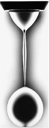
Figure 1: A drop of Glycerin dripping through Polydimethylsiloxane near pinch-off [5]. The nozzle diameter is $0.48$ cm, the viscosity ratio is $\lambda=0.95$.

A fascinating aspect of the study of singularities is that they describe a great variety of phenomena which appear in the natural sciences and beyond [3]. Some examples of such singular events occur in free-surface flows [6], turbulence and Euler dynamics (singularities of vortex tubes [7, 8] and sheets [9]), elasticity [10], Bose-Einstein condensates [11], non-linear wave physics [12], bacterial growth [13, 14], black-hole cosmology [15, 16], and financial markets [17].

In this paper we consider evolution equations

$$h_{t}=F[h],$$ (1.1)

where $F[h]$ represents some (nonlinear) differential or integral operator. We will also discuss cases where $h$ is a vector, and thus (1.1) is a system of equations. Furthermore, the spatial variable $x$ may also have several dimensions, and thus potentially different scaling in different coordinate directions. We will cite some examples below, but few of the higher-dimensional cases have so far been analysed in detail. For the purpose of the following discussion, let us suppose that both $x$ and $h$ are scalar quantities, and that the singularity occurs at a single point in space and time $x_{0},t_{0}$. If $t^{\prime}=t_{0}-t$ and $x^{\prime}=x-x_{0}$, we are looking for local solutions of (1.1) which have the structure

$$h(x,t)=t^{\prime\alpha}H(x^{\prime}/t^{\prime\beta}),$$ (1.2)

with appropriately chosen values of the exponents $\alpha,\beta$. Note that later the prime is also used to indicate a derivative. However, this will always be with respect to a spatial variable like $x,z$, or the similarity variable $\xi$, hence confusion should not arise.

Giga and Kohn [18, 19] proposed to introduce self-similar variables $\tau=-\ln(t^{\prime})$ and $\xi=x^{\prime}/t^{\prime\beta}$ to study the asymptotics of blow up. Namely, putting

$$h(x,t)=t^{\prime\alpha}H(\xi,\tau),$$ (1.3)

(1.1) is turned into the “dynamical system”

$$H_{\tau}=G[H]\equiv\alpha H-\beta\xi H_{\xi}+F[H].$$ (1.4)

By virtue of (1.4), solutions to the original PDE (1.1) for given initial data can be viewed as orbits in some infinite dimensional phase phase, for instance, $L^{2}$. To understand the blow-up of (1.1), Giga and Kohn proposed to study the long-time behaviour of the dynamical system (1.4). Thus in particular, one is interested in the attractors of (1.4) ($\omega$-limit sets in the notation which is customary in the context of partial differential equations, see [20] and references therein). If (1.2) is indeed a solution of (1.1), the right hand side of (1.4) is independent of $\tau$, and self-similar solutions of the form (1.2) are fixed points of (1.4), which we will denote by $\overline{H}(\xi)$. By studying the dynamics close to the fixed point, we find that the dynamical system (1.4) frequently reduces to very few dimensions. Thus on one hand one obtains detailed information on the behaviour of the original problem (1.1) near blowup. On the other hand, one also gains a fruitful means of classifying, or at least characterising singularities.

The most basic linear stability analysis of this self-similar solution consists in linearising around the fixed point according to

$$H=\overline{H}(\xi)+\epsilon P(\xi,\tau),$$ (1.5)

which gives

$$P_{\tau}={\cal L}P,$$ (1.6)

where ${\cal L}\equiv{\cal L}(\overline{H})$ depends on the fixed point solution $\overline{H}$. To solve (1.6), we write $P$ as a superposition of eigenfunctions $P_{j}$ of the operator ${\cal L}$:

$$P(\xi)=\sum_{j=1}^{\infty}a_{j}(\tau)P_{j}(\xi),$$ (1.7)

where $\nu_{j}$ is the eigenvalue:

$${\cal L}P_{j}=\nu_{j}P_{j}.$$ (1.8)

In the cases we know, the spectrum turns out to be discrete. For evolution PDE’s involving second order elliptic differential operators, such as semilinear parabolic equations, mean curvature or Ricci flows, the discreteness of the spectrum of the linearisation about the fixed point is a direct consequence of Sturm-Liouville theory [21, 22]. This theory establishes that, under quite general conditions on the coefficients of a second order linear differential operator and the boundary conditions, its spectrum is discrete and the corresponding eigenfunctions form a complete set in a suitably weighed $L^{2}$ space. Some explicit examples are presented in subsection 3.1.1. For general linear operators such a theory is not available, and one has to study the spectrum case by case.

Now the solution of (1.6) corresponding to $P_{j}$ is

$$P=e^{\nu_{j}\tau}P_{j},$$ (1.9)

and all eigenvalues need to be negative for the similarity solution to be stable. In that case, convergence to the fixed point is exponential, or algebraic in the original time variable $t^{\prime}$. Soon the solution has effectively reached the fixed point, and there is very little change in the self-similar behaviour. If one or several of the eigenvalues around the fixed point vanish, the approach to the fixed point is slow, and the dynamics is effectively described by a dynamical system whose dimension corresponds to the number of vanishing eigenvalues. The same holds true if the attractor has few dimensions (such as a limit cycle or a low-dimensional chaotic attractor). Thus although singular behaviour is in principle a problem to be solved in infinite dimensions, in practise it typically reduces to a dynamical problem of few dimensions. In this review we analyse singularities from the point of view of the slow dynamics contained in (1.4), to obtain an overview and tentative classification of possible scaling behaviours. We also emphasise the physical significance of these different types of behaviours.

The perspective described above suggests a close relationship to the description of scaling phenomena by means of the renormalisation group, developed in the context of critical phenomena [23, 24]; we will continue to point out similarities, but we are not aware that a classification similar to ours has been achieved using the language of the renormalisation group. For a computational perspective on analysing (1.4) in terms of its slow dynamics, see [25]. Finally, another approach sometimes associated with the classification of singularities is catastrophe theory [26]. However, as far as we are aware catastrophe theory only yields useful results if the problem can be mapped onto a low-dimensional geometrical problem, which can in turn be rephrased in terms of normal forms of polynomials. This has been shown to be the case for wave problems such as shock formation and wave breaking [27], as well as singularities of the eikonal equation [28] and related problems [29].

In this paper we discuss the following cases:

1. Stable fixed points (section 2)

   In this case the fixed point is approached exponentially in the logarithmic variable $\tau$, so the dynamics is described by the self-similar law (1.2). This pure power-law behaviour is also known as type-I self-similarity [30].

2. Centre manifold (section 3)

   Here one or more of the eigenvalues around the fixed point are zero. As a result, the approach to the fixed point is only algebraic, leading to logarithmic corrections to scaling. This is called type-II self-similarity [30]; it characterises cases where the blow-up rate is different from what is expected on the basis of a solution of the type (1.2).

3. Travelling waves (section 4)

   Solutions of (1.1) converge to $h=t^{\prime\alpha}\phi(\xi+c\tau)$, which is a travelling wave solution of (1.4) with propagation velocity $c$.

4. Limit cycles (section 5)

   Solutions have the form $h={t^{\prime}}^{\alpha}\mathbf{\psi}\left[\xi,\tau\right]$ with $\psi$ being a periodic function of period $T$ in $\tau$. This is known as “discrete self-similarity” [15, 31], since at times $\tau_{n}=\tau_{0}+nT$, n integer, the solution looks like a self-similar one.

5. Strange attractors (section 6)

   The dynamics on scale $\tau$ are described by a nonlinear (low-dimensional) dynamical system, such as the Lorenz equation.

6. Multiple singularities (section 7)

   Blow-up may occur at several points $(x_{0},t_{0})$ (or indeed in any set of positive measure), in which case the description (1.4) is not useful. We also describe cases where (1.2) still applies, and blow-up occurs at a single point, but the underlying dynamics is really one of two singularities which merge at the singular time.

Equation	Type	Dynamics	Section
Free surface flow
$h_{t}+\nabla\cdot(h^{n}\nabla\triangle h)\pm\nabla(h^{p}\nabla h)=0$	I,II	stable ?	2.1.1
$(h^{2})_{t}+(h^{2}u)_{x}=0$	I
$\rho(u_{t}+uu_{x})=(h^{2}u_{x})_{x}/h^{2}-(h^{-1})_{x}$		stable	2.1.1
$h_{t}=\left[h\kappa_{x}/(1+h_{x}^{2})^{1/2}\right]_{x},$	I
$\kappa=1/(h(1+h_{x}^{2})^{1/2})-h_{xx}/(1+h_{x}^{2})^{3/2}$		stable	2.1
$h_{t}+(hu)_{x}=0,\quad u_{t}+uu_{x}=h_{xxx}$	I	stable	2.4.2
$\int\frac{\ddot{a}(\xi,t)d\xi}{\sqrt{(x-\xi)^{2}+a(x,t)}}=\frac{\dot{a}^{2}}{2a}$	II	$v_{\tau}=-v^{3}$	3.2.1
$u(x)=\frac{1}{4}\int\frac{h_{z}(z)}{\sqrt{h^{2}(z)+(x-z)^{2}}}dz$
$(h^{2})_{t}+(h^{2}u)_{x}=0$	III	stable	4
Geometric evolution equations
$h_{t}=h_{zz}/(1+h_{z}^{2})-1/h$	II	$u_{\tau}=-u^{2}$	3.1.1
$\psi_{t}=\psi_{ss}-(n-1)(1-\psi_{s}^{2})/\psi$	II	$u_{\tau}=-u^{2}$	3.1.1
Reaction-diffusion equations
$u_{t}-\triangle u=f(u)$	II	$u_{\tau}=-u^{2}$	3.1.2
$u_{t}-\nabla\cdot(|u|^{m}\nabla u)=u^{p}$	II	unknown	3.1.2
$\rho_{t}+\nabla\cdot(\rho\nabla S-\nabla\rho)=0,\quad\rho=-\triangle S$	II	$u_{\tau}=-u^{3}$	3.2.2
Nonlinear dispersive equations
$u_{t}+uu_{x}=0$	I	stable	2.4
$i\psi_{t}+\triangle\psi+|\psi|^{p}\psi=0$	I,II	$u_{\tau}=-u^{2}/v$
		$v_{\tau}=-uv$	3.3
$u_{t}+u^{p}u_{x}+u_{xxx}=0$	II	unknown	3.3.1
$u_{t}-u_{xxt}+3uu_{x}=2u_{x}u_{xx}+uu_{xxx}$	I	unknown	3.3.1
$u_{t}=2fv,\quad v_{t}=-2fu,\quad f_{t}=f^{2}$	IV	circle	5
Choptuik equations	I, IV	limit cycle	5
$u_{tt}=u_{xx}+|u|^{p}u$	I,II	unknown	7.2
Fluid equations
$u_{t}+(u\cdot\nabla)u=-\nabla p+\triangle u,\quad\nabla\cdot u=0$	I, IV ?	unknown	2.2
$u_{t}+(u\cdot\nabla)u=-\nabla p,\quad\nabla\cdot u=0$	I, IV ?	unknown	2.2
$u_{t}+uu_{x}+vu_{y}=-p_{x}+u_{yy},\quad u_{x}+v_{y}=0$	I	stable	2.2

Table 1: A summary of PDE’s discussed in this paper. The first column gives the PDE in question, the second the type of dynamics near the fixed point according to the classification enumerated above. In the case of attracting fixed-point dynamics, it is classed as “stable”, otherwise the equation governing the slow dynamics is given.

This paper’s aim is to assemble the body of knowledge on singularities of equations of the type (1.1) that is available in both the mathematical and the applied community, and to categorise it according to the types given above. In addition to rigorous results we pay particular attention to various phenomenological aspects of singularities which are often crucial for their appearance in an experiment or a numerical simulation. For example, what are the observable implications of the convergence onto the self-similar form (1.2) being slow? In most cases, we rely on known examples from the literature, but the problem is almost always reformulated to conform with the formulation advocated above. However, some examples are entirely new, which we will indicate as appropriate. For each of the above categories, we will present at least one example in greater detail, so the analysis can be followed explicitely. A concise overview of the equations presented in this review is given in Table 1.

2 Stable fixed points

A sub-classification into self-similarity of the first and second kind has been expounded in [32, 33, 34, 35]. Self-similar solutions are of the first kind if (1.2) only solves (1.1) for one set of exponents $\alpha,\beta$; their values are fixed by either dimensional analysis or symmetry, and are thus rational. Solutions are of the second kind if solutions (1.2) exist locally for a continuous set of exponents $\alpha,\beta$; however, in general these solutions are inconsistent with the boundary or initial conditions. Imposing these conditions leads to a non-linear eigenvalue problem, whose solution yields irrational exponents in general.

2.1 Self-similarity of the first kind

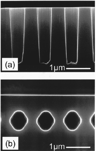
Figure 2: SEM images illustrating the pinch-off of a row of rectangular troughs in silicon (top) [36]. The bottom picture shows the same sample after 10 minutes of annealing at $1100^{\circ}$C. The troughs have pinched off to form a row of almost spherical voids. The dynamics is driven by surface diffusion.

Our example, exhibiting self-similarity of the first kind [35], is that of a solid surface evolving under the action of surface diffusion. Namely, atoms migrate along the surface driven by gradients of chemical potential, see Fig.2. The resulting equations in the axisymmetric case, where the free surface is described by the local neck radius $h(x,t)$, are [37]:

$$h_{t}=\frac{1}{h}\left[\frac{h}{(1+h_{x}^{2})^{1/2}}\kappa_{x}\right]_{x},$$ (2.1)

where

$$\kappa=\frac{1}{h(1+h_{x}^{2})^{1/2}}-\frac{h_{xx}}{(1+h_{x}^{2})^{3/2}}$$ (2.2)

is the mean curvature. In (2.1),(2.2), all lengths have been made dimensionless using an outer length scale $R$ (such as the initial neck radius), and the time scale $R^{4}/D_{4}$, where $D_{4}$ is a forth-order diffusion constant.

Physically, it is important to point out that (2.1) describes the evolution of the free surface at elevated temperatures, above the so-called roughening transition. This implies that the solid surface is smooth and does not exhibit facets, coming from the underlying crystal structure. Above the roughening transition, a continuum description is still possible [38]. The study of these models has lead to a number of interesting similarity solutions describing singular behaviour of the surface, such as grooves [39] or mounds [40, 41].

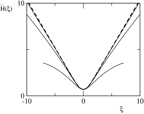
Figure 3: The approach to the self-similar profile for equation (2.1). The dashed line is the stable similarity solution $H(\xi)$ as found from (2.4). The full lines are rescaled profiles found from the original dynamics (2.1) at $h_{m}=10^{-1},10^{-2}$, and $h_{m}=10^{-3}$, respectively. As the singularity is approached, they converge rapidly onto the similarity solution (2.3).

At a time $t^{\prime}\ll 1$ away from breakup, dimensional analysis implies that $\ell=t^{\prime 1/4}$ is a local length scale. This suggests the similarity form

$$h(x,t)=t^{\prime 1/4}H(x^{\prime}/t^{\prime 1/4}),$$ (2.3)

and thus the exponents $\alpha,\beta$ of (1.2) are fixed by dimensional analysis, which is typical for self-similarity of the first kind. Of course, the result (2.3) also follows when directly searching for a solution of (2.1) in the form of (1.2). In other cases, a unique set of local scaling exponents is determined by symmetry [42]. The similarity form of the PDE becomes

$$-\frac{1}{4}(H-\xi H_{\xi})=\frac{1}{H}\left[\frac{H}{(1+H_{\xi}^{2})^{1/2}}\kappa_{\xi}\right]_{\xi},\quad\xi=\frac{x^{\prime}}{t^{\prime 1/4}}$$ (2.4)

where $\kappa$ is the mean curvature of $H$.

Solutions of (2.4) have been studied extensively in [43]. To ensure matching to a time-independent outer solution, the leading order time dependence must drop out from (2.3), implying that

$$H(\xi)\sim c|\xi|,\quad\xi\rightarrow\pm\infty;$$ (2.5)

the general form of this matching condition for self-similar solutions of the form (1.2) is

$$H(\xi)\sim c|\xi|^{\frac{\alpha}{\beta}},\quad\xi\rightarrow\pm\infty.$$ (2.6)

All solutions of the similarity equation (2.1), and which obey the growth condition (2.5) are symmetric, and form a discretely infinite set [43], similar to a number of other problems discussed below. The series of similarity solutions is conveniently ordered by descending values of the minimum, see table 2. Only the lowest order solution $H_{0}(\xi)$ is stable, and is shown in Fig. 3; we return to the issue of stability in section 2.5 below. The fact that permissible similarity solutions form a discrete set implies a great deal of “universality” in the way pinching can occur. It means that the local solution is independent of the outer solution, and rather that the former imposes constraints on the latter; in particular, the prefactor $c$ in (2.5) must be determined as part of the solution (see Table 2).

i	$H_{i}(0)$	$c_{i}$
0	0.701595	1.03714
1	0.636461	0.29866
2	0.456842	0.18384
3	0.404477	0.13489
4	0.355884	0.10730
5	0.326889	0.08942

Table 2: A series of similarity solutions of (2.4) as given in [43]. The higher-order solutions become successively thinner and flatter.

2.1.1 Thin films and thin jets

A further class of solutions displaying self-similarity of the first kind is the generalised long-wave thin-film equation

$$h_{t}+\nabla\cdot(h^{n}\nabla\Delta h-Bh^{m}\nabla h)=0\ ,\ n>0.$$ (2.7)

The mass flux in this equation has two contributions: the first is due to surface tension, and the second is due to an external potential. When $n=m=3$, then $z=h(\mathbf{x},t)$ represents the height of a film or a drop of viscous fluid over a flat surface, located at $z=0$; the external potential is gravity. If $B$ is negative, (2.7) describes a film that is hanging from a ceiling. Regardless of the sign of $B$, there is no singularity in this case [44]. The case $n=1$ and $B=0$ corresponds to flow between two solid plates, to which we return in section 7.1 below.

Solutions to (2.7) are said to develop point singularities if $h$ goes to zero in finite time. This happens if one incorporates van der Waals forces, which at leading order implies $n=3$ and $m=-1$ with $B<0$. In [45], [46] (see also the review [47], where further full numerical simulations and mathematical theory are reported) the existence of radially symmetric self-similar touchdown solutions of the form

$$h(r,t)=t^{\prime\frac{1}{5}}H(\xi),\quad\xi=r/t^{\prime\frac{2}{5}}$$ (2.8)

is shown numerically in this case. Self-similar solutions that touch down along a line exist as well, but they are unstable. A proof of formation of singularities in this context has been provided by Chou and Kwong [48].

A related set of equations are those for thin films and jets, but which are isolated instead of being in contact with a solid. Problems of this sort furnish many examples of type-I scaling, as reviewed from a physical perspective in [49]. If the motion is no longer dampened by the presence of a solid, inertia often has to be taken into account. This means that a separate equation for the velocity is needed, which is essentially the Navier-Stokes equation below, but often simplified by a reduction to a single dimension. Thus one has solutions of the form

$$h(x,t)=t^{\prime\alpha}H(\xi),\quad u(x,t)=t^{\prime\beta-1}U(\xi),$$ (2.9)

where $\xi=x^{\prime}/t^{\prime\beta}$. If $\alpha>\beta$ the profile is slender, and the dynamics is well described in a shallow-water theory. In this case the equations for an axisymmetric jet with surface tension become

$$\partial_{t}h^{2}+\partial_{x}(uh^{2})=0$$ (2.10)

and

$$\rho(\partial_{t}u+u\partial_{x}u)=-(\gamma/\rho)\partial_{x}(1/h)+3\nu\frac{\partial_{x}(\partial_{x}uh^{2})}{h^{2}}.$$ (2.11)

The system (2.10),(2.11) is interesting because it exhibits different scaling behaviours depending on the balance between the three different terms in (2.11) [42]. This is an illustration of the principle of dominant balance, which is of great practical importance in practise, where it is a priori not known which physical effect will be dominant. In the case of (2.11), these are the forces of inertia on the left, surface tension (first term on the right), and viscosity (second term on the right). Pinching is driven by surface tension, so it must always be part of the balance. Three different possible balances remain [42]:

(i) In the first case [50], all forces in (2.11) are balanced as the singularity is approached. The exponents $\alpha=1,\beta=1/2$ in (2.9) follow directly from this condition. As shown in [51], there is a discretely infinite sequence of self-similar profiles $H(\xi),U(\xi)$ corresponding to this balance. Numerical evidence strongly suggests that only the first profile, corresponding to the thickest thread, is stable [6]. All the other profiles are unstable, and thus cannot be observed. We will revisit this general scenario again below, when we study the stability of fixed points more generally.

(ii) The second possibility corresponds to a balance between surface tension and viscous forces, thus putting $\rho=0$ in (2.11). Physically, this occurs if the fluid is very viscous [52]. In section 2.4.1 below we will describe the pinching solution corresponding to this case in more detail, as an example of self-similarity of the second kind. The exponent $\alpha=1$ is fixed by the balance, but $\beta$ is fixed only by an integrability condition. This once more results in an infinite sequence of solutions, ordered by the value of $\beta$. Again, only one profile, which has the largest value of $\beta=0.17487$ is stable. This time, this corresponds to the smallest value of the minimum radius $R_{0}$, or the thinnest thread, as opposed to thickest thread in the case of the inertial-surface tension-viscous balance.

If one inserts this viscous solution into the original equation (2.11), one finds that in the limit $t^{\prime}\rightarrow 0$, the inertial term on the left grows faster than the two terms on the right. This means that regardless how large the viscosity, eventually all three terms become of the same order, and one observes a crossover to the inertial-surface tension-viscous similarity solution described above, which is characterised by another set of scaling exponents and similarity profiles. In particular, the surface tension-viscous solution is symmetric about the pinch point, whereas the solution containing inertia is highly asymmetric [53]. We remark that crossover between different similarity solutions may also occur by another mechanism, not directly related to the dominant balance between different terms in the equation (cf. section 7.1).

Equations (2.10),(2.11) correspond to a viscous liquid, surrounded by a gas, which is not dynamically active. The case of an external viscous fluid is considered in detail in section 4 below. The case of no internal fluid is special, in that the dynamics decouples completely into one for independent slices [54]. As a result, there is no universal profile associated with the breakup of a bubble in a viscous environment, but rather it is determined by the initial conditions.

(iii) At very low viscosity ($\nu\approx 0$ in (2.11)), the relevant balance is one where inertia is balanced by surface tension, so one might want to set $\nu=0$ in (2.11), as done originally in [55]. However, the resulting equations do not lead to a selection of the values of the scaling exponents $\alpha,\beta$; instead, there is a continuum of solutions [56], parameterised by the value of $\alpha$, each with a continuum of possible similarity profiles. In fact, for vanishing viscosity (2.10),(2.11) does not go toward a pinching solution, but the slope of the interface steepens, and one finds a shock solution [57], similar to the generic scenario described in section 2.4 below.

It was however shown numerically in [58, 59], and investigated in more detail in [60], that pinch-off of an inviscid fluid is well described by a solution of the full three-dimensional, axisymmetric potential flow equations. This is thus an example of a similarity solution of higher order in the independent variable, but both coordinate directions scale in the same way. The scaling exponents in (2.9) are $\alpha=\beta=2/3$ in this case, which violates the assumption $\alpha>\beta$ for the validity of the shallow water equations (2.10),(2.11). In addition, we note that the similarity profile can no longer even be written as a graph as assumed in (2.9), but turn over, as first observed experimentally in [61]. It is not known whether there also exists a sequence of similarity solutions, as in the case of the other balances. The case of no internal fluid is again very special, and leads to type-II scaling. It is considered in section 3.2.1 below.

Finally, variations of (2.10),(2.11) have been investigated in [62]. Breakup was considered in arbitrary dimensions $d$ (yet retaining axisymmetry) and with the pressure term $1/h$ replaced by an arbitrary power law $1/h^{p}$. After introducing a new variable $1/h^{p}$, there remains a single parameter $r=(d-1)/p$, which can formally be varied continuously. For all values of $r$, discrete sequences of type-I solutions are obtained. For $r>1/2$, profiles are asymmetric, while below that value they are symmetric. At the critical value, both types of solutions coexist. Another interesting feature of the limit $r=1/2$ is that the viscous term becomes subdominant at leading order. However, similar to the case $d=3,p=1$ mentioned above, no selection takes place in the absence of the viscous term. Nevertheless, the solutions selected by the presence of the viscous term are very close to an appropriately chosen member of the family of inviscid solutions.

2.2 Singularities in Euler and Navier-Stokes equations

One of the most important open problems, both in physics and mathematics, is the existence of singularities in the equations of fluid mechanics: Euler and Navier-Stokes equations in three space dimensions. The Navier-Stokes equations represent the evolution of a viscous incompressible fluid and are of the form

$$\mathbf{u}_{t}+\mathbf{u}\cdot\nabla\mathbf{u}=-\nabla p+Re^{-1}\Delta\mathbf{u},\qquad\nabla\cdot\mathbf{u}=0,$$ (2.12)

where $\mathbf{u}$ represents the velocity field, $p$ the pressure in the fluid and Re is a dimensionless parameter called Reynolds number. Formally, by making Re$\rightarrow\infty$, the term involving $\Delta\mathbf{u}$ vanishes and we arrive at the Euler system, that models the evolution of the velocity and pressure fields of an inviscid incompressible fluid:

$$\mathbf{u}_{t}+\mathbf{u}\cdot\nabla\mathbf{u}=-\nabla p,\qquad\nabla\cdot\mathbf{u}=0.$$ (2.13)

We exclude from our discussion certain “exact” blow-up solutions of the Euler equations [63], which have the defect that the velocity goes to infinity uniformly in space; in other words, they lack the crucial mechanism of focusing. Formally, they are of course similarity solutions of (2.13), but with spatial exponent $\alpha=0$.

As we mentioned above, the existence of singular solutions is unknown. Nevertheless, some scenarios have been excluded. For the Navier-Stokes equations, there exists no nontrivial self-similar solution of the first kind

$$\mathbf{u}(\mathbf{x},t)=t^{\prime-1/2}\mathbf{U}\left(\mathbf{\xi}\right),\quad\mathbf{\xi}={\bf x}^{\prime}/t^{\prime 1/2}$$ (2.14)

in $L^{2}(\mathbb{R}^{3})$. This was proved by Necas, Ruzicka and Sverak [64]. However, this does not exclude the formation of a singularity in a localised region: the matching condition (2.6) for this case implies $|{\bf U}|\propto|\xi|^{-1}$ as $|\xi|\rightarrow\infty$, which is not in $L^{2}$. Therefore, the theorem [64] does not apply.

A possible self-similar solution consisting of two skewed vortex-pairs has been proposed by Moffatt in [7] in the spirit of the scenario suggested by the numerical simulations of Pelz [65], of the implosion of six vortex pairs in a configuration with cubic symmetry. More recent numerical experiment by Hou and Li [66] seem to indicate that, although the velocity field may grow to very large values, singularities in the above mentioned scenarios saturate eventually and the solutions remain smooth. It has been argued in [67] that no self-similar solutions for Euler system should exist and that the ”limit-cycle” scenario described in section 5 could apply.

Under certain circumstances, such as special symmetry conditions or appropriate asymptotic limits, the Navier-Stokes and Euler systems may simplify and give rise to models for which the question of existence of singular solutions is somewhat simpler to analyse. This is the case for the Prandtl boundary-layer equations for the 2-D evolution of the velocity field $(u,v)$ in $y\geq 0$:

$$u_{t}+uu_{x}+vu_{y}=-p_{x}+u_{yy},\quad u_{x}+v_{y}=0$$ (2.15)

with boundary conditions $u=v=0$; $p$ is a given pressure field and the behaviour of the velocity field at infinity is prescribed. Equation (2.15) describes the asymptotic limit of the Navier-Stokes equation near a solid body in the limit of large Reynolds numbers $Re$. The variable $x$ measures the arclength along the body, and $Re^{1/2}y$ is the distance from the body. Historically, a lot of attention was focused on the stationary version of (2.15), considering it as an evolution equation in $x$. At some position $x_{s}$ along the body, the so-called Goldstein singularity $v\propto(x_{s}-x)^{-1/2}$ is encountered [68], which signals separation of the flow from the body. However, in reality the outer flow changes as a result of the appearance of a stagnation point, and one has to consider the interaction between the boundary layer and the outer flow [69].

It is thus conceptually simpler to consider the case of unsteady boundary layer separation, which is described by the first singularity of (2.15) at time $t_{0}$. The formation of singularities of (2.15) in finite time was proved by E and Engquist [70]. It was first found numerically by van Dommelen and Shen [71], and its analytical structure was investigated in [72], using Lagrangian variables, which follow fluid particles as they separate from the surface (see also [73]). In the original Eulerian variables, the self-similar structure is [74, 75]

$$u=-u_{0}+t^{\prime 1/2}\phi_{0}^{1/2}U(\xi,\eta),\quad\xi=\frac{x^{\prime}-u_{0}t^{\prime}}{t^{\prime 3/2}\phi_{0}^{1/2}},\;\eta=\frac{y\phi_{0}^{1/4}}{t^{\prime 1/4}\Lambda},$$ (2.16)

where $u_{0},\phi_{0}$, and $\Lambda$ are constants which depend on the problem, while $U$ is universal and can be given in terms of elliptic integrals. Note that the exponents for $u$ and $x$ are the generic exponents for a developing shock (see section 2.4 below), while the similarity exponent in the $y$-direction is different from the scaling for two-dimensional breaking waves [27]. We stress that the appearance of a singularity in (2.15) does not mean that the full 2D Navier-Stokes equation has developed a singularity. Instead, lower order terms in the asymptotic expansion that lead to (2.15) become important close to the singularity.

In relation with singularities in fluid mechanics, we can mention briefly a few important problems involving models or suitable approximations to the original Euler and Navier-Stokes systems. One concerns weak solutions to the Euler system for which the vorticity ($\omega=\nabla\times\mathbf{u}$) is concentrated in curves or surfaces. This is the case of the so called vortex filaments and sheets in which the vorticity remains concentrated for all times, in absence of viscosity. A useful way to represent the vortex sheet, when it evolves in 2D, is by assuming the location of its points $(x(\alpha,t),y(\alpha,t))$ as complex numbers $z(\alpha,t)=x(\alpha,t)+iy(\alpha,t)$. Then, the evolution of $z(\alpha,t)$ is given by the so-called Birkhoff-Rott equation [76]:

$$z_{t}^{\ast}(\alpha,t)=\frac{1}{2\pi i}PV\int_{-\infty}^{\infty}\frac{\gamma(z(\alpha^{\prime},t),t)}{z(\alpha,t)-z(\alpha^{\prime},t)}z_{\alpha}(\alpha^{\prime},t)d\alpha^{\prime}\ ,$$ (2.17)

where $z^{\ast}$ stands for the complex conjugate of $z$. The principal value is denoted by PV, and $\gamma$ is the vortex strength and is such that $d\Gamma=\gamma(z(\alpha,t),t)z_{\alpha}(\alpha,t)d\alpha$ is constant along particle paths of the flow. The question then is whether or not these geometrical objects will remain smooth at all times or develop singularities in finite time. In the case of vortex sheets, singularities are known to develop in the form of a divergence of the curvature at some point. These are called Moore’s singularities after their observation and description by D. W. Moore [77]. A mathematical proof of existence of these singularities is provided by Caflisch and Orellana in [78]. These singularities exhibit self-similarity of the first kind as shown, for instance, in [79]: if one defines the inclination angle $\theta(s,t)$ in terms of the arclength parameter $s$ as such that $z_{s}=e^{i\theta}$, then the curvature is given by $\kappa=\theta_{s}$ and may blow-up in the self-similar form (up to multiplicative constants):

$$\kappa(s,t^{\prime})=\frac{1}{t^{\prime\delta}}g(\eta),\quad\eta=s^{\prime}/t^{\prime}\ ,\ \ 0<\delta<1,$$ (2.18)

where

$$g(\eta)=\frac{1}{(1+\eta^{2})^{\frac{\delta}{2}}}\sin(\delta\arctan\eta)\ .$$ (2.19)

Interestingly, numerical simulations and Moore’s original observations suggest that, although singular solutions with any $\delta$ are possible, that the solution with $\delta=\frac{1}{2}$ is preferred. Thus the generically observed geometry near the singularity is of the form $y=\left|x\right|^{\frac{3}{2}}$, including the case of 3D simulations. This poses an interesting ”selection problem” for the $\frac{3}{2}$ power which has not received a definitive answer so far.

Another type of solution of (2.17) has the from of a double-branched spiral vortex sheet [80]. The explicit form is

$$z(\beta,t)=\left\{\begin{array}[]{l}t^{\prime q}\beta^{\nu}\quad\beta>0\\ t^{\prime q}|\beta|^{\nu}\quad\beta<0\quad\;,\end{array}\right.$$ (2.20)

where the two cases correspond to the two branches of the spiral. The parameter $\beta$ is related to integration variable $\alpha$ of (2.17) by $d\beta=z_{\alpha}d\alpha$. The exponents are of the form $\nu=1/2+ib$ and $q=1/2+i\mu b$, corresponding to a vortex of radius $r=t^{\prime 1/2}$ collapsing in finite time. However, in this case the vortex sheet strength is found to increase exponentially at infinity [80].

Vortex filaments result as the limit of a vortex tube when the thickness tends to zero. The fluid flow around a vortex filament is frequently approximated by a truncation of the Biot-Savart integral for the velocity in terms of the vorticity. This leads to a geometric evolution equation for the filament (see [81], chapter 7, and references therein) that can be transformed, via Hasimoto transformation, into the cubic Nonlinear-Schrödinger in 1D. This fact allowed Gutierrez, Rivas and Vega to construct exact self-similar solutions for infinite vortex filaments [82]. One can also consider the vorticity concentrated in a region separating two fluids of different density and in the presence of gravitational forces. This is the case of the surface water waves system for which the existence of singularities is open [83].

A different approach in the study of singularities for Euler and Navier-Stokes equations in three space dimensions relies on the development of models that share some of the essential mathematical difficulties of the original systems, but in a lower space dimension. This is the case of the surface quasi-geostrophic equation popularised by Constantin, Majda and Tabak [84]:

$$\theta_{t}+{\bf v}\cdot\nabla\theta=0,$$ (2.21a)

$${\bf v}=\nabla^{\bot}\psi,\quad\theta=-(-\triangle)^{1/2}\psi,$$ (2.21b)

to be solved in $d=2$. This system of equations describes the convection of an active scalar $\theta$, representing the temperature, with a velocity field which is an integral operator of the scalar itself. Nevertheless, the mere existence of singular solutions to this equation in the form of blow-up for the gradient of $\theta$ is still an open problem. One-dimensional analogues of this problem, representing the convection of a scalar with a velocity field, which is the Hilbert transform of the scalar itself do have singularities in the form of cusps, as proved in [85], [86]. The structure of such singularities has been described in [87] and they are, in fact, of the type described in the next section, that is of the second kind.

2.3 Self-similarity of the second kind

In the example of the previous subsection, the exponents can be determined by dimensional analysis, or from considerations of symmetry, and therefore assume rational values. In many other problems, however, the scaling behaviour depends on external parameters, set for example by the initial conditions. In that case, the scaling exponent can assume any value. Often, this value is fixed by a compatability condition, resulting in an irrational answer. We will call this situation self-similarity of the second kind [32, 35]. Since it is relatively rare that results are tractable analytically, we mention two simple examples for which this is possible, although they do not come from time-dependent problems.

The first example is that of viscous flow near a solid corner of opening angle $2\alpha$ [88]. For analogues of this problem in elasticity, see [89, 90] as well as the discussion in [35]. This flow is described by a Stokes’ equation, whose solution near the corner is expected to be

$$\psi=r^{\lambda}f_{\lambda}(\theta).$$ (2.21v)

If one of the boundaries is moving, scaling is of the first kind, and $\lambda=2$ (the so-called Taylor scraper [91]). However, if the flow is driven by two-dimensional stirring at a distance from the corner, $\lambda$ is determined by the transcendental equation

$$\sin 2(\lambda-1)\alpha=-(\lambda-1)\sin 2\alpha.$$ (2.21w)

If $2\alpha<146^{\circ}$, (2.21w) admits complex solutions, which correspond to an infinite sequence of progressively smaller corner eddies. Since $\lambda$ is complex, The strength of the eddies decreases as one comes closer to the corner.

The second example consists in calculating the electric field between two non-conducting spheres, where an external electric field is applied in the direction of the symmetry plane [92]. In this case the electric potential between the spheres is proportional to $(\rho/(Rh))^{\sqrt{2}-1}$, where $\rho$ is the radial distance from the symmetry axis, $R$ the sphere radius, and $h$ the distance between the spheres. Thus in accordance with the the general ideas of self-similarity of the second kind, the singular behaviour is not controlled by the local quantity $\rho/h$, but the “outer” parameter $R$ comes into play as well. We now explain two analytically tractable dynamical examples of self-similarity of the second kind.

2.4 Breaking waves in conservation laws

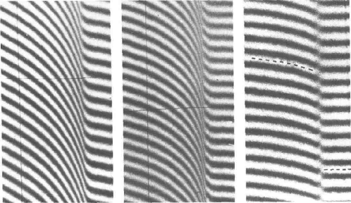
Figure 4: Fringe pattern showing the steepening of a wave in a gas, leading to the formation of a shock, which is travelling from left to right [93]. The vertical position of a given fringe is proportional to the density at that point. In the last picture a jump of seven fringes occurs.

We only consider the simplest model for the formation of a shock wave in gas dynamics, which is Burger’s equation

$$u_{t}+uu_{x}=0.$$ (2.21x)

It is generally believed that any system of conservation laws that exhibits blow up will locally behave like (2.21x) [94]. For example, Fig. 4 shows the steepening of a density wave in a gas, leading to a jump of the density in the picture on the right. In the words of [93]: “We conclude that an infinite slope in the theoretical solution corresponds to a shock in real life”. As throughout this review, we only consider the dynamics up to the singularity. Which structure emerges after the singularity depends on the regularisation used, as the continuation to times after the singularity is not unique [95, 96]. If the regularisation is diffusive, a shock wave forms [97]; if it is a third derivative, one finds a KDV soliton. Finally, regularisation by higher-order nonlinearities has been considered in [27] as a model of wave breaking.

It is well known [98] that (2.21x) can be solved exactly using the method of characteristics. This method consists in noting that the velocity remains constant along the characteristic curve

$$z=u_{0}(x)t+x,$$ (2.21y)

where $u_{0}(x)=u(x,0)$ is the initial condition. Thus

$$u(z,t)=u_{0}(x)$$ (2.21z)

is an exact solution to (2.21x), given implicitly.

It is geometrically obvious that whenever $u_{0}(x)$ has a negative slope, characteristics will cross in finite time and produce a discontinuity of the solution. This happens when $\partial z/\partial x=0$, which will occur for the first time at the singularity time

$$t_{0}=\min\left\{-\frac{1}{\partial_{x}u_{0}(x)}\right\},$$ (2.21aa)

at a spatial position $x=x_{m}$. This means a singularity will first form at

$$x_{0}=x_{m}-\frac{u_{0}(x_{m})}{\partial_{x}u_{0}(x_{m})}.$$ (2.21ab)

Since (2.21x) is invariant under any shift in velocity, we can assume without loss of generality that $u_{0}(x_{m})=0$, and thus that $x_{0}=x_{m}$. This means the velocity is zero at the singularity. We now analyse the formation of the singularity using the local coordinates $x^{\prime},t^{\prime}$. In [27], this was done by expanding the initial condition $u_{0}$ in $x^{\prime}$, and using (2.21z), using ideas from catastrophe theory [26]. Here instead we use the similarity ideas developed in this paper.

The local behaviour of (2.21x) near $t_{0}$ can be obtained using the scaling

$$u(x,t)=t^{\prime\alpha}U\left(x^{\prime}/t^{\prime\alpha+1}\right),$$ (2.21ac)

which solves (2.21x). The similarity equation becomes

$$-\alpha U+(1+\alpha)\xi U_{\xi}+UU_{\xi}=0,$$ (2.21ad)

with implicit solution

$$\xi=-U-CU^{1+1/\alpha}.$$ (2.21ae)

The special case $\alpha=0$ has the solution $U=-\xi$, which is inconsistent with the matching condition (2.6), and thus has to be discarded.

We are thus left with a continuum of possible scaling exponents $\alpha>0$, as is typical for self-similarity of the second kind. A discretely infinite sequence of exponents $\alpha_{n}$ is however selected by the requirement that (2.21ae) defines a smooth function for all $\xi$. Namely, one must have $1+1/\alpha$ odd, or

$$\alpha_{i}=\frac{1}{2i+2},\quad i=0,1,2\dots,$$ (2.21af)

and we denote the corresponding similarity profile by $U_{i}$. The constant $C$ in (2.21ae) must be positive, but is otherwise arbitrary. It is set by the initial conditions, which is another hallmark of self-similarity of the second kind. However, $C$ can be normalised to 1 by rescaling $x$ and $U$. We will see in section 2.5 that the solution with $\alpha_{0}$,

$$u(x,t)=t^{\prime 1/2}U_{0}\left(x^{\prime}/t^{\prime 3/2}\right),$$ (2.21ag)

is the only stable one, all higher-order solutions are unstable.

It is interesting to look at some possible exceptions to the form of blow-up given above, suggested by [94]:

$$u_{t}+uu_{x}=u^{\sigma}.$$ (2.21ah)

This equation is also solved easily using characteristics. For $\sigma\leq 2$ the blow-up is alway of the form (2.21ag), for $\sigma>2$ two different behaviours are possible. For small initial data $u_{0}(x)$, a singularity still forms like (2.21ag), but in addition $u$ may also go to infinity. However, there is a boundary between the two behaviours [94], where the slope blows up at the same time that $u$ goes to infinity. For this case, one expects all terms in (2.21ah) to be of the same order, giving

$$u(x,t)=t^{\prime\frac{1}{1-\sigma}}U\left(\xi)\right),\quad\xi=x^{\prime}/t^{\prime\frac{\sigma-2}{\sigma-1}},$$ (2.21ai)

with similarity equation

$$\frac{U}{1-\sigma}+\frac{\sigma-2}{\sigma-1}\xi U_{\xi}=U^{\sigma}-UU_{\xi}.$$ (2.21aj)

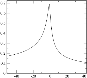
Figure 5: The similarity solution (2.21ak) for $\sigma=4$.

The solution to (2.21aj) that has the right decay at infinity is

$$\xi=-\frac{1}{(\sigma-2)U^{\sigma-2}}\pm C\frac{\left(1-(\sigma-1)U^{\sigma-1}\right)^{\frac{\sigma-2}{\sigma-1}}}{U^{\sigma-2}},$$ (2.21ak)

where $C>0$ is an arbitrary constant. The + and - signs describe the solution to the right and left of $\xi^{*}=-(\sigma-1)^{\frac{\sigma-2}{\sigma-1}}/(\sigma-2)$, respectively. The special case $\sigma=4$ is shown in Fig. 5. The similarity solution (2.21ak) is not smooth at its maximum; rather, its first derivative behaves like $U_{\xi}\propto(\xi-\xi^{*})^{1/(\sigma-2)}$. This can be understood from the exact solution; in order for blow-up to occur at the same time that a shock is formed, the initial profile must already have a maximum with the same regularity as (2.21ak). Thus, the situation leading to (2.21ai) is a very special one, requiring very peculiar initial conditions.

2.4.1 Viscous pinch-off

As explained in section 2.1.1, the pinch-off of a very viscous fluid is described by (2.10), (2.11), with $\rho=0$, but only for finite range of scales. The equations can be simplified considerably by introducing Lagrangian variables, i.e. writing all profiles as a function of a particle label $s$. This means the particle is at position $z(s,t)$ at time $t$, and $z_{t}(s,t)$ is the velocity at time $t$. The jet profile can be obtained from $z_{s}=1/h^{2}(s,t)$, and (2.11) becomes

$$h_{t}(s,t)=\frac{1}{6}\left(1+\frac{C(t)}{h(s,t)}\right).$$ (2.21al)

The typical velocity scale is $\gamma/\eta$, where $\gamma$ is the surface tension and $\eta$ is the viscosity; (2.21al) has been made dimensionless accordingly. The time-dependent constant of integration $C(t)$ has to be determined self-consistently. Note that the self-similar form (1.2) is a solution of (2.21al) for $\alpha=1$, and any value of $\beta$; the exponent $\beta$ will be determined by the consistency condition (2.21as) below.

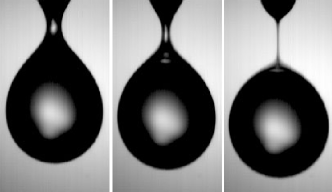
Figure 6: A drop of viscous fluid falling from a pipette 1 mm in diameter [99]. Note the long neck.

Since $\alpha=1$, a scaling solution of (2.21al) has the form

$$h^{-2}(s,t)=t^{\prime-2}f\left(\xi\right),\quad\mbox{with}\quad\xi=s^{\prime}/t^{\prime\gamma}$$ (2.21am)

and

$$C(t)=-C_{0}t^{\prime}\ .$$ (2.21an)

The relationship with the exponent $\beta$ defined in (2.9) is simply $\beta=\gamma-2$, as found from passing from Lagrangian to Eulerian variables. Inserting (2.21am),(2.21an) into (2.21al) we obtain

$$\frac{1}{\sqrt{f}}+3\left(\frac{2}{f}+\frac{\gamma\xi f_{\xi}}{f^{2}}\right)=C_{0},$$ (2.21ao)

where $C_{0}$ is a constant. Imposing symmetry and regularity of $f$, we expand $f(\xi)$ in the form

$$f_{i}(\xi)=R_{0}^{-2}+\xi^{2i+2}+O(\xi^{2i+4})\ ,\ i=0,1,2,\dots$$ (2.21ap)

where we have normalised the coefficient of $\xi^{2i+2}$ to one. This is consistent, since any solution of (2.21al) is only determined up to a scale factor. Instead, the axial scale is fixed by the initial conditions. The parameter $R_{0}$ is the rescaled minimum of the profile: $h_{m}=R_{0}t^{\prime}$. Inserting (2.21ap) into (2.21ao), at order $\xi^{2i+2}$ one obtains

$$R_{0}=\frac{1}{12(\overline{\gamma}-1)},\quad C_{0}=\frac{1}{24}\frac{2\overline{\gamma}-1}{(\overline{\gamma}-1)^{2}}$$ (2.21aq)

where we have put $\overline{\gamma}=(i+1)\gamma$.

Each choice of $i$ corresponds to one member in an infinite sequence of similarity solutions. Equation (2.21ao) can easily be integrated in terms of $\ln\xi$ and $y=\sqrt{f}$:

$$\int\frac{dy}{\left(\left(1+6R_{0}\right)y^{3}-y^{2}-6R_{0}y\right)}=\frac{1}{6R_{0}\gamma}\ln\xi+\widetilde{C}=\frac{1}{6R_{0}\overline{\gamma}}\ln\xi^{i+1}+\widetilde{C},$$

with $\widetilde{C}$ an arbitrary constant. Computing the integral above we obtain

$$y^{-\overline{\gamma}}\left(\left(2\overline{\gamma}-1\right)y+1\right)^{\overline{\gamma}-\frac{1}{2}}\left(1-y\right)^{\frac{1}{2}}=\xi^{i+1},$$ (2.21ar)

which is an implicit equation for the i-th similarity profile $y\equiv y_{i}(\xi)=\sqrt{f_{i}(\xi)}$.

The value of the velocity $U_{\infty}$ at infinity must be a constant to be consistent with boundary conditions. It can be found by integrating $z_{ts}=(h^{-2})_{t}=t^{\prime-3}(2f+\gamma\xi f_{\xi})$ from zero to infinity:

$$U_{\infty}=\int_{0}^{\infty}z_{ts}ds=\frac{t^{\prime\gamma-3}}{3}\int_{0}^{\infty}\left(\left(\frac{1}{24}\frac{2\overline{\gamma}-1}{(\overline{\gamma}-1)^{2}}\right)f^{2}-f^{\frac{3}{2}}\right)d\xi=0,$$ (2.21as)

where we have used (2.21ao). The above condition $U_{\infty}=0$, which ensures that $U_{\infty}$ does not diverge as $t^{\prime}\rightarrow 0$, is the equation which determines the exponent $\gamma$. Taking the derivative of (2.21ar) we obtain

$$(i+1)\xi^{i}\frac{d\xi}{dy}=\frac{d}{dy}\left(y^{-\overline{\gamma}}\left(\left(2\overline{\gamma}-1\right)y+1\right)^{\overline{\gamma}-\frac{1}{2}}\left(1-y\right)^{\frac{1}{2}}\right)=$$

$$=-y^{-\overline{\gamma}-1}\left(2y\overline{\gamma}-y+1\right)^{\overline{\gamma}-\frac{3}{2}}\frac{\overline{\gamma}}{\sqrt{\left(1-y\right)}}$$

which can be used to transform the integral in (2.21as) to the variable $y$:

$$K_{i}(\gamma)\equiv\frac{3U_{\infty}}{(12(\overline{\gamma}-1))^{3}}=\frac{\overline{\gamma}}{i+1}\int_{0}^{1}\left(\left(\frac{1}{2}\frac{2\overline{\gamma}-1}{\overline{\gamma}-1}\right)y^{4}-y^{3}\right)\cdot$$

$$\left(y^{-\frac{i+1+\overline{\gamma}}{i+1}}\left(\left(2\overline{\gamma}-1\right)y+1\right)^{-\frac{1}{2}\frac{2i-2\overline{\gamma}+3}{i+1}}\left(1-y\right)^{-\frac{1}{2}\frac{2i+1}{i+1}}\right)dy=0.$$ (2.21at)

The function $K_{i}(\gamma)$ may be written explicitly as

$$K_{i}(\gamma)=\gamma\frac{\Gamma\left(4-\gamma\right)\Gamma\left(\frac{1}{2i+2}\right)}{\Gamma\left(4-\gamma+\frac{1}{2i+2}\right)}\left(\frac{1}{2}\frac{(2i+2)\gamma-1}{(i+1)\gamma-1}\right)\cdot$$

$$F\left(\frac{2i+3}{2i+2}-\gamma,4-\gamma;4-\gamma+\frac{1}{2i+2};1-(2i+2)\gamma\right)-\gamma\frac{\Gamma\left(3-\gamma\right)\Gamma\left(\frac{1}{2i+2}\right)}{\Gamma\left(3-\gamma+\frac{1}{2i+2}\right)}\cdot$$

$$F\left(\frac{2i+3}{2i+2}-\gamma,3-\gamma;3-\gamma+\frac{1}{2i+2};1-(2i+2)\gamma\right),$$ (2.21au)

where $F(a,b;c,z)$ is the hypergeometric function [100]. Roots of $\gamma_{i}$ are given in Table 3.

To summarise, each exponent $\gamma_{i}$ corresponds to a new member $f_{i}(\xi)$ of an infinite hierarchy of similarity profiles, to be found from (2.21ar). If one converts the Lagrangian variables back to the original spatial variables, one obtains

$$h(x,t)=t^{\prime}\phi^{(n)}_{St}\left(x^{\prime}/t^{\prime\gamma-2}\right).$$ (2.21av)

Thus for $t^{\prime}\rightarrow 0$ the typical radial scale $t^{\prime}$ of the generic $i=0$ solution rapidly becomes smaller than the axial scale $t^{\prime 0.175}$ (cf. Table 3). This explains the long necks seen in Fig. 6.

i	$\gamma_{i}$	$R_{0}$
0	2.1748	0.0709
1	2.0454	0.0797
2	2.0194	0.0817
3	2.0105	0.0825
4	2.0065	0.0828
5	2.0044	0.0832

Table 3: A list of exponents, found from $K_{i}(\gamma)=0$ using MAPLE, with $K_{i}$ given by (2.21au). The number $2i+2$ gives the smallest non-vanishing power in a series expansion of the corresponding similarity solution around the origin. Only the solution with $i=0$ is stable. The rescaled minimum radius is found from (2.21aq).

2.4.2 More examples

Other recent examples for scaling of the second kind have been observed for the breakup of a two-dimensional sheet with surface tension. In a shallow-water approximation, which is justified for a description of breakup, the equations read [101]

$$h_{t}+(hu)_{x}=0,\quad u_{t}+uu_{x}=h_{xxx}$$ (2.21aw)

after appropriate rescaling. Local similarity solutions can be found in the form

$$h(x,t)=t^{\prime 4\beta-2}H(\eta),\quad u(x,t)=t^{\prime\beta-1}U(\eta),$$ (2.21ax)

where $\eta=x^{\prime}/t^{\prime\beta}$. The exponent $\beta$ is not determined by dimensional analysis. Instead, it must be found from a solvability condition on the nonlinear system of equations for the similarity functions $H,U$.

The result of the numerical calculation is [101] $\beta=0.6869\pm 0.0003$, which is curiously close to $\beta=2/3$, which is the value that had been conjectured earlier [102], but contains a small correction. The value $\beta=2/3$ comes out if both length scales in the longitudinal and transversal directions are assumed to be the same, implying that $4\beta-2=\beta$. This is a natural expectation for problems governed by Laplace’s equation, such as inviscid, irrotational flow [59], and indeed is observed for three-dimensional drop breakup [58, 59]. However, in present case, even if the full two-dimensional irrotational flow equations are used, $\beta\neq 2/3$.

Other physical problems which frequently involve anomalous scaling exponents are strong explosions on one hand, and collapse of particles or gases into a singular state on the other. These types of problems have been reviewed in great detail in a number of textbooks and articles [32, 34, 33, 35], but continue to attract a great deal of attention. As with many other singular problems, the type of scaling depends on the details of the underlying physics, and scaling of both the first and second kind is observed. For example, the radius of a shock wave resulting from a strong explosion can be calculated from dimensional analysis to be $r_{s}\propto t^{2/5}$ [103]. However, in the seemingly analogous case of a strong implosion, an anomalous exponent is observed, which moreover depends on the parameters of the problem [104, 98]. Cases were collapse and shock formation coincide were given by [105] (similar to section 2.4 above). In a somewhat different context, anomalous scaling is observed in model calculations for the collapse of self-gravitating particles [106] and Bose-Einstein condensates [107]. It is important to remember that these examples come from kinetic equations describing the stochastic collision of waves or particles, and hence involving nonlocal collision operators. However, the kinetic equations appear to be closely related to certain PDE problems [108], which are analogous to other evolution equations studied in this article.

2.5 Stability of fixed points

Self-similar solutions correspond to fixed points of the dynamical system (1.4), whose stability we now investigate by linearising around the fixed point. We explain the situation for the example of section 2.1 in more detail, for which the transformation reads

$$h(x,t)=t^{\prime 1/4}H(\xi,\tau),$$ (2.21ay)

where $\tau=-\ln(t^{\prime})$. The similarity form of (2.1) becomes

$$H_{\tau}=\frac{1}{4}(H-\xi H_{\xi})+\frac{1}{H}\left[\frac{H}{(1+H_{\xi}^{2})^{1/2}}\kappa_{\xi}\right]_{\xi},$$ (2.21az)

which reduces to (2.4) if the left hand side is set to zero. To assure matching of (2.21az) to the outer solution, we have to require that (2.21ay) is to leading order time-independent as $\xi$ is large, which leads to the boundary condition

$$H_{\tau}-(H-\xi H_{\xi})/4\rightarrow 0\quad\mbox{for}\quad|\xi|\rightarrow\infty.$$ (2.21ba)

This is the natural extension of (2.5) to the time-dependent case.

Next we linearise around any one of the similarity solutions $\overline{H}(\xi)=H_{i}(\xi)$ listed in Table 2, as described in the Introduction. The stability is controlled by eigenvalues of the eigenvalue equation (1.8). Inserting the eigensolution (1.9) into (2.21ba) one finds that $P_{j}$ must grow at infinity like

$$P_{j}(\xi)\propto\xi^{1-4\nu_{j}}.$$ (2.21bb)

Similarly, the growth condition for the general case of a similarity solution of the form (1.2) is

$$P_{j}(\xi)\propto\xi^{\frac{\alpha-\nu_{j}}{\beta}}.$$ (2.21bc)

If the similarity solution $\overline{H}(\xi)$ is to be stable, the real part of the eigenvalues of ${\cal L}$ must be negative. However, there are always two positive eigenvalues, which are related to the invariance of the equation of motion (2.1) under translations in space and time, as noted by [109, 110]. Namely, for any $\epsilon$, the translated similarity solution

$$h^{(\epsilon)}(x,t)=t^{\prime 1/4}\overline{H}(\frac{x^{\prime}+\epsilon}{t^{\prime 1/4}})$$ (2.21bd)

is an equally good self-similar solution of (2.1), and thus of (2.21az). In particular, we can expand (2.21bd) to lowest order in $\epsilon$, and find that

$$H^{(\epsilon)}(\xi,\tau)=\overline{H}(\xi)+\epsilon e^{\beta\tau}\overline{H}_{\xi}(\xi)+O(\epsilon^{2}),$$ (2.21be)

where the linear term is a solution of (1.6).

Thus

$$\left(e^{\beta\tau}\overline{H}_{\xi}\right)_{\tau}=e^{\beta\tau}\beta\overline{H}_{\xi}=e^{\beta\tau}{\cal L}\overline{H}_{\xi}.$$ (2.21bf)

But this means that $\nu_{x}=\beta\equiv 1/4$ is an eigenvalue of ${\cal L}$ with eigenfunction $\overline{H}_{\xi}(\xi)$. Similarly, considering the transformation $t\rightarrow t+\epsilon$, one finds a second positive eigenvalue $\nu_{t}=1$, with eigenfunction $\xi\overline{H}_{\xi}$. However, these two positive eigenvalues do not correspond to instability. Instead, the meaning of these eigenvalues is that upon perturbing the similarity solution, the singularity time as well as the position of the singularity will change. Thus if the coordinate system is not adjusted accordingly, it looks as if the solution would flow away from the fixed point. If, on the other hand, the solution is represented relative to the perturbed values of $x_{0}$ and $t_{0}$, the eigenvalues $\nu_{x}$ and $\nu_{t}$ will not appear.

The eigenvalue problem (1.8) was studied numerically in [43]. It was found that each similarity solution $\overline{H}_{i}$ has exactly $2i$ positive real eigenvalues, disregarding $\nu_{x},\nu_{t}$. The result is that the linearisation around the “ground state” solution $\overline{H}_{0}$ only has negative eigenvalues while all the other solutions have at least one other positive eigenvalue. This means that $\overline{H}_{0}$ is the only similarity solution that can be observed, all other solutions are unstable. Close to the fixed point, the approach to $\overline{H}_{0}$ will be dominated by the largest negative eigenvalue $\nu_{1}$:

$$h(x,t)=t^{\prime 1/4}\left[\overline{H}(\xi)+\epsilon t^{\prime-\nu_{1}}P_{1}(\xi)\right].$$ (2.21bg)

For large arguments, the point $\xi_{cr}$ where the correction becomes comparable to the similarity solution is $\xi\sim\epsilon t^{\prime-\nu_{1}}\xi^{1-4\nu_{1}}$, and thus $\xi_{cr}\sim t^{\prime-1/4}$. This means that the region of validity of $\overline{H}(\xi)$ expands in similarity variables, and is constant in real space. This rapid convergence is reflected by the numerical results reported in Fig. 3. More formally, one can say that for any $\epsilon$ there is a $\delta$ such that

$$\left|h(x,t)-t^{\prime 1/4}\overline{H}(\xi)\right|\leq\epsilon$$ (2.21bh)

if $|x^{\prime}|\leq\delta$ uniformly as $t^{\prime}\rightarrow 0$.

We suspect that the situation described above is more general: the ground state is stable, while each following profile has a number of additional eigenvalues. In the case of the sequence of profiles $\overline{H}_{i}$ of (2.4), two new positive eigenvalues appear for each new profile, corresponding to a symmetric and an antisymmetric eigenfunction. Below we give two more examples of the same scenario, for which we are able to give a simple geometrical interpretation for the appearance of two additional positive eigenvalues at each stage of the hierarchy of similarity solutions. The simplest case is that of shock wave formation (cf. section 2.4), for which everything can be worked out analytically.

The dynamical system corresponding to the self-similar solution (2.21ac) is

$$U_{\tau}-\alpha U+\left(1+\alpha\right)\xi U_{\xi}+UU_{\xi}=0,$$ (2.21bi)

and so the eigenvalue equation for perturbations $P$ around the base profile $\overline{U}_{i}$ becomes

$$(\alpha_{i}-\nu)P-(1+\alpha_{i})\xi P_{\xi}-P(\overline{U}_{i})_{\xi}-P_{\xi}\overline{U}_{i}=0,\quad i=0,1,\dots$$ (2.21bj)

Here $\overline{U}_{i}$ is the ith similarity function defined by (2.21ae) for the exponents $\alpha_{i}$ as given by (2.21af).

The eigenvalue equation (2.21bj) is solved easily by transforming from the variable $\xi$ to the variable $\overline{U}$, using (2.21ae):

$$P\left[(\alpha_{i}-\nu)(1+(2i+3)\overline{U}_{i}^{2i+2})+1\right]=\frac{\partial P}{\partial\overline{U}}\left[\alpha_{i}\overline{U}_{i}+(1+\alpha_{i})\overline{U}_{i}^{2i+3}\right],$$ (2.21bk)

with solution

$$P=\frac{\overline{U}_{i}^{3+2i-2\nu(i+1)}}{1+(2i+3)\overline{U}_{i}^{2i+2}}.$$ (2.21bl)

The exponent $3+2i-2\nu(i+1)$ must be an integer for (2.21bl) to be regular at the origin, so the eigenvalues are

$$\nu_{j}=\frac{2i+4-j}{2i+2},\quad j=1,2,\dots$$ (2.21bm)

As usual, the eigensolutions are alternating between even and odd. However, we are interested in the first instance, given by (2.21aa), at which a shock forms. This implies that the second derivative of the profile must vanish at the location of the shock, and the amplitude of the $j=3$ perturbation must be exactly zero.

Thus for $i=0$ the remaining eigenvalues are $\nu=3/2,1,0,-1/2,\dots$; the first two are the eigenvalues $\nu_{x}=\beta=1+\alpha$ and $\nu_{t}=1$ found above. The vanishing eigenvalue occurs because there is a family of solutions parameterised by the coefficient $C$ in (2.21ae). All the other eigenvalues are negative, which shows that the similarity solution (2.21ag) is stable. In the same vein, for $\alpha_{1}=1/4$ there are two more positive exponents: $\nu=5/4,1,1/2,1/4$, so the solution must be unstable. The same is of course true for all higher order solutions. Thus in conclusion the ground state solution $\overline{U}_{0}$ given by (2.21ag) is the only observable form of shock formation. The same conclusion was reached in [27] by a stability analysis based on catastrophe theory.

The sequence of profiles for viscous pinch-off, found in section 2.3, suggests a simple mechanism for the fact that two new unstable directions appear with each new similarity profile of higher order. In fact, the argument is strikingly similar to that given for shock formation. Differentiating (2.21al) with respect to $s$ one finds that a local minimum point $s_{min}$ remains a minimum. Thus the local time evolution of the profile can be written as

$$h(s,t)=h_{m}+\sum_{j=2}^{\infty}B_{j}(t)s^{\prime j}.$$ (2.21bn)

For generic initial data $B_{2}(0)\neq 0$, so there is no reason why $B_{2}$ should vanish at the singular time, which means that the self-similar solution $f_{0}$ will develop, which has a quadratic minimum. This situation is structurally stable, so one expects the eigenvalues of the linearisation to be negative. If however the coefficients $B_{j}(0)$ are zero for $j=2,\dots 2n-1$, they will remain zero for all times. Namely, if the first $k$ $s$-derivatives of $h$ vanish, one has

$$\partial_{s}^{j}h_{t}=-\frac{C\partial_{s}^{j}h}{h^{2}},\quad j=1,\dots,k,$$ (2.21bo)

so the first $k$ derivatives will remain zero. Thus to find the similarity profile with $i=1$, one needs $B_{2}(0)=B_{3}(0)=0$ as an initial condition. This is a non-generic situation, and a slight perturbation will make $B_{2}$ and $B_{3}$ nonzero. In other words, there are two unstable directions, which take the solution away from $f_{1}(\xi)$, as defined by (2.21ap). In the general case, the linearisation around $f_{i}(\xi)$ will have $2i$ positive eigenvalues (apart from the trivial ones). Extensive numerical simulations of drop pinch-off in the inertial-surface tension-viscous regime (cf. section 2.1.1) suggests that the the hierarchy of similarity solutions again has similar properties in this case as well, although stability has not been studied theoretically. The ground-state profile is stable, while all the others are unstable [42]. Even when using a higher-order similarity solution as an initial condition, it is immediately destabilised, and converges onto the ground state solution [51].

3 Centre manifold

In section 2 we described the generic situation that the behaviour of a similarity solution is determined by the linearisation around it. In the case of a stable fixed point, convergence is exponentially fast, and the observed behaviour is essentially that of the fixed point. In this section, we describe a variety different cases where the the dynamics is slow. In all cases we are able to associate this slow dynamics with a fixed point in the appropriate variable(s), around which the eigenvalues vanish. Instead, higher-order non-linear terms have to be taken into account, and the slow approach to the fixed point is determined by a low-dimensional dynamical system.

We consider essentially two different cases:

• The dynamical system (1.4) possesses a fixed point $H_{0}(\xi)$, which has a vanishing eigenvalue, with corresponding eigenfunction $\psi(\xi)$. The dynamics in the slow direction $\psi$ is described by a nonlinear equation for the amplitude $a(\tau)$, which varies on a logarithmic time scale:

  $$h=t^{\prime\alpha}\left[H_{0}(\xi)+a(\tau)\psi(\xi)\right],\quad\xi=x^{\prime}/t^{\prime\beta}.$$ (2.21a)

• The dynamical system does not possess a fixed point, but has a solution of a slightly more general form:

  $$h=h_{0}(\tau)H(\xi),\quad\xi=x^{\prime}/W(\tau),$$ (2.21b)

  where $h_{0}$ and $W$ are not necessarily power laws. To expand about a fixed point, we define the generalised exponents

  $$\alpha=-\partial_{\tau}h_{0}/h_{0},\quad\beta=-\partial_{\tau}W/W$$ (2.21c)

  which now depend on time. In the case of a type-I similarity solution, this reduces to the usual definition of the exponent. In the cases considered below, one derives a finite dimensional dynamical system for the exponents $\alpha,\beta$ (potentially including other, similarly defined scale factors). Once more, the exponents vary on a logarithmic time scale, which can be understood from the fact that the dynamical system possesses a fixed point with vanishing eigenvalues.

Zero eigenvalues can also be associated to symmetries of the singularity, like rotational or translational symmetries, which lead to the existence of a continuum of similarity solutions. Another example, which concerns the dynamics inside the singular object itself, is wave steepening as described by (2.21ae) above. As seen from (2.21bm), there indeed is a vanishing eigenvalue associated with this continuum of solutions. Below we will not be concerned with this case, but only consider approach to the singularity starting from nonsingular solutions.

3.1 Quadratic non-linearity: geometric evolution and reaction-diffusion equations

The appearance of this type of nonlinearity is characteristic for various nonlinear parabolic equations and systems. The blow-up behaviour is characterised by the presence of logarithmic corrections in the similarity profiles.

3.1.1 Geometric evolution equations: Mean curvature and Ricci flows

Axisymmetric motion by mean curvature in three spatial dimensions is described by the equation

$$h_{t}=\left(\frac{h_{xx}}{1+h_{x}^{2}}-\frac{1}{h}\right),$$ (2.21d)

where $h(x,t)$ is the radius of the moving free surface. A very good physical realization of (2.21d) is the melting and freezing of a ³He crystal, driven by surface tension [111], see Fig. 7. As before, the time scale $t$ has been chosen such that the diffusion constant, which sets the rate of motion, is normalised to one. A possible boundary condition for the problem is that $h(0,t)=h(L,t)=R$, where $R$ is some prescribed radius. For certain initial conditions $h(x,0)\equiv h_{0}(x)$ the interface will become singular at some time $t_{0}$, at which $h(x_{0},t_{0})=0$ and the curvature blows up. The moment of blow-up is shown in panel h of Fig. 7, for example.

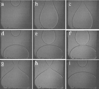
Figure 7: Nine images (of width 3.5 mm) showing how a ³He crystal “flows” down from the upper part of a cryogenic cell into its lower part [112]. The recording takes a few minutes, the temperature is 0.32 K. 11 mK. The crystal first “drips” down, so that a crystalline “drop” forms at the bottom (a to c); then a second drop appears (d) and comes into contact with the first one (e); coalescence is observed (f) and subsequently breakup occurs (h).

Inserting the self-similar solution (1.2) into (2.21d), one finds a balance for $\alpha=\beta=1/2$. The corresponding similarity equation is

$$-\frac{\phi}{2}+\xi\frac{\phi_{\xi}}{2}=\left(\frac{\phi_{\xi\xi}}{1+\phi_{\xi}^{2}}-\frac{1}{\phi}\right),\quad\xi=\frac{x^{\prime}}{t^{\prime 1/2}}.$$ (2.21e)

One solution of (2.21e) is the constant solution $\phi(\xi)=\sqrt{2}$. Another potential solution is one that grows linearly at infinity, to ensure matching onto a time-independent outer solution. However, it can be shown that no solution to (2.21e), which also grows linearly at infinity, exists [113, 114]. Our analysis below follows the rigorous work in [30], demonstrating type-II self-similarity. In addition, we now show how the description of the dynamical system can be carried out to arbitrary order.

The relevant solution is thus the constant solution, but which of course does not match onto a time-independent outer solution. We thus write the solution as

$$h(x,t)=t^{\prime 1/2}\left[\sqrt{2}+g(\xi,\tau)\right],$$ (2.21f)

with $\tau=-\ln(t^{\prime})$ as usual. The equation for $g$ is then

$$g_{\tau}=g-\frac{\xi g_{\xi}}{2}+\frac{g_{\xi\xi}}{1+g_{\xi}^{2}}-\frac{g^{2}}{2^{3/2}+2g},$$ (2.21g)

which we solve by expanding into eigenfunctions of the linear part of the operator

$${\cal L}g=g-\xi g_{\xi}/2+g_{\xi\xi}.$$ (2.21h)

It is easily confirmed that

$${\cal L}H_{2i}(\xi/2)=\nu_{i}H_{2i}(\xi/2),\quad i=0,1,\dots,$$ (2.21i)

where $H_{n}$ is the n-th Hermite polynomial [100]:

$$H_{n}(y)=(-1)^{n}e^{y^{2}}\frac{d^{n}}{dy^{n}}e^{-y^{2}},$$ (2.21j)

and $\nu_{i}=1-i$. Thus the first eigenvalue is $\nu_{0}=1$, which corresponds to the positive eigenvalue $\nu_{t}$ coming from the arbitrary choice of $t_{0}$. The other positive eigenvalue eigenvalue $\nu_{x}$ does not appear, since we have chosen to look at symmetric solutions, breaking translational invariance. However, the largest non-trivial eigenvalue $\nu_{1}$ is zero, and the linear part of (2.21g) becomes

$$\frac{\partial a_{i}}{\partial\tau}=(1-i)a_{i},\quad i=0,1,\dots.$$ (2.21k)

Thus all perturbations with $i>1$ decay, but to investigate the approach of the cylindrical solution, one must include nonlinear terms in the equation for $a_{1}$.

If we write

$$g(\xi,\tau)=\sum_{i=1}^{\infty}a_{i}(\tau)H_{2i}(\xi/2),$$ (2.21l)

the equation for $a_{1}$ becomes

$$\frac{da_{1}}{d\tau}=-2^{3/2}a_{1}^{2}+O(a_{1}a_{j}),$$ (2.21m)

whose solution is

$$a_{1}=1/(2^{3/2}\tau).$$ (2.21n)

Thus instead of the expected exponential convergence onto the fixed point, the approach is only algebraic. Since all other eigenvalues are negative, the $\tau$-dependence of the $a_{i}$ is slaved by the dynamics of $a_{1}$. Namely, as we will see below, $a_{j}=O(\tau^{-j})$, so corrections to (2.21m) are of higher order. To summarise, the leading-order behaviour of (2.21d) is given by

$$h(x,t)=t^{\prime 1/2}\left[\sqrt{2}+a_{1}(\tau)H_{2}(\xi)\right],$$ (2.21o)

as was proven by [30].

Now we compute the specific form of the higher-order corrections to (2.21o), which have not been worked out explicitly before. If one linearises around (2.21n), putting $a_{1}=a_{1}^{(0)}+\epsilon_{1}$, one finds

$$\frac{d\epsilon_{1}}{d\tau}=-\frac{2}{\tau}\epsilon_{1}+\mbox{other terms}.$$ (2.21p)

This means that the coefficient $A$ of $\epsilon_{1}=A/\tau^{2}$ remains undetermined, and a simple expansion of $a_{i}$ in powers of $\tau^{-1}$ yields an indeterminate system. Instead, at quadratic order, a term of the form $\epsilon_{1}=A\ln\tau/\tau^{2}$ is needed. Fortunately, this is the only place in the system of nonlinear equations for $a_{i}$ where such an indeterminacy occurs. Thus all logarithmic dependencies can be traced, leading to the general ansatz

$$a_{i}^{(n)}=\frac{\delta_{i}}{\tau^{i}}+\sum_{k=i+1}^{n}\sum_{l=0}^{k-i}\frac{(\ln\tau)^{l}}{\tau^{k}}\delta_{lki},$$ (2.21q)

where $\delta_{i}$ and $\delta_{lki}$ are coefficients to be determined. The index $n$ is the order of the truncation.

The coefficients can now be found recursively by considering terms of successively higher order in $\tau^{-1}$ in the first equation:

$$\frac{da_{1}}{d\tau}=-2^{3/2}a_{1}^{2}-24\sqrt{2}a_{1}a_{2}+22a_{1}^{3}-$$

$$272\sqrt{2}a_{1}^{4}-191\sqrt{2}a_{2}^{2}+192a_{1}^{2}a_{2}$$ (2.21ra)

$$\frac{da_{2}}{d\tau}=-a_{2}-\sqrt{2}/4a_{1}^{2}+6a_{1}^{3}-8\sqrt{2}a_{1}a_{2}.$$ (2.21rb)

The next two orders will involve the next coefficient $a_{3}$. From (2.21ra) and (2.21rb), one first finds $\delta_{121}$ and $\delta_{2}$, by considering $O(\tau^{-3})$ and $O(\tau^{-2})$, respectively. Then, at order $O(\tau^{-(n+1)})$ in the first equation, where $n=3$, one finds all remaining coefficients $\delta_{lki}$ in the expansion (2.21q) up to $k=n$. At each order in $\tau^{-1}$, there is of course a series expansion in $\ln\tau$ which determines all the coefficients.

We constructed a MAPLE program to compute all the coefficients up to arbitrarily high order (10th, say). Up to third order in $\tau^{-1}$ the result is:

$$a_{1}=1/4\,{\frac{\sqrt{2}}{\tau}}+{\frac{17}{16}}\,{\frac{\ln\left(\tau\right)\sqrt{2}}{{\tau}^{2}}}-{\frac{73}{16}}\,{\frac{\sqrt{2}}{{\tau}^{3}}}+$$

$${\frac{867}{128}}\,{\frac{\ln\left(\tau\right)\sqrt{2}}{{\tau}^{3}}}-{\frac{289}{128}}\,{\frac{\left(\ln\left(\tau\right)\right)^{2}\sqrt{2}}{{\tau}^{3}}}$$ (2.21rsa)

$$a_{2}=-1/32\,{\frac{\sqrt{2}}{{\tau}^{2}}}+{\frac{5}{16}}\,{\frac{\sqrt{2}}{{\tau}^{3}}}-{\frac{17}{64}}\,{\frac{\ln\left(\tau\right)\sqrt{2}}{{\tau}^{3}}},$$ (2.21rsb)

and thus $h(x,t)$ becomes

$$h(x,t)=t^{\prime 1/2}\left[\sqrt{2}+a_{1}(\tau)\left(-2+\xi^{2}\right)+a_{2}(\tau)\left(12-12\xi^{2}+\xi^{4}\right)\right],$$ (2.21rst)

from which one of course immediately finds the minimum. To second order, the result is

$$h_{m}=(2t^{\prime})^{1/2}\left[1-\frac{1}{2\tau}-\frac{3+17\ln\tau}{8\tau^{2}}\right].$$ (2.21rsu)

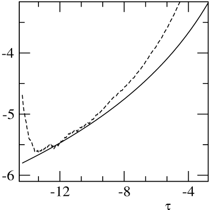
Figure 8: A plot of $\left[h_{m}/\sqrt{2t^{\prime}}-1+1/(2\tau)\right]\tau^{2}$ (dashed line) and $\tau_{0}/2-(3+17\ln(\tau+\tau_{0})/8)$ (full line) with $\tau_{0}=4.56$.

First, the presence of logarithms implies that there is some dependence on initial conditions built into the description. The reason is that the argument inside the logarithm needs to be non-dimensionalised using some “external” time scale. More formally, any change in time scale $\tilde{t}=t/t_{0}$ leads to an identical equation if also lengths are rescaled according to $\tilde{h}=h/\sqrt{t_{0}}$. This leaves the prefactor in (2.21rsu) invariant, but adds an arbitrary constant $\tau_{0}$ to $\tau$. This is illustrated by comparing to a numerical simulation of the mean curvature equation (2.21d) close to the point of breakup, see Fig. 8. Namely, we subtract the analytical result (2.21rsu) from the numerical solution $h_{m}/(2\sqrt{t^{\prime}})$ and multiply by $\tau^{2}$. As seen in Fig.8, the remainder is varying slowly over 12 decades in $t^{\prime}$. If the constant $\tau_{0}$ is adjusted, this small variation is seen to be consistent with the logarithmic dependence predicted by (2.21rsu).

The second important point is that convergence in space is no longer uniform as implied by (2.21bh) for the case of type I self-similarity. Namely, to leading order the pinching solution is a cylinder. For this to be a good approximation, one has to require that the correction is small: $\xi^{2}/\tau\ll 1$. Thus corrections become important beyond $\xi_{cr}\sim\tau$, which, in view of the logarithmic growth of $\tau$, implies convergence in a constant region in similarity variables only. As shown in [111], the slow convergence toward the self-similar behaviour has important consequences for a comparison to experimental data.

Mean curvature flow is also an example of a broader class of problems called generically ”geometric evolution equations”. These are evolution equations intended to gain topological insight by flowing geometrical objects (such as metric or curvature) towards easily recognisable objects such as constant or positive curvature manifolds. The most remarkable example is the so called Ricci flow, introduced in [115], which is the essential tool in the recent proof of the geometrisation conjecture (including Poincaré’s conjecture as a consequence) by Grigori Perelman.

Namely, Poincaré’s conjecture states that every simply connected closed 3-manifold is homeomorphic to the 3-sphere. Being homeomorphic means that both are topologically equivalent and can be transformed one into the other through continuous mappings. Such mappings can be obtained from the flow associated to an evolutionary PDE involving fundamental geometrical properties of the manifold. Thurston’s geometrisation conjecture is a generalisation of Poincaré’s conjecture to general 3-manifolds and states that compact 3-manifolds can be decomposed into submanifolds that have basic geometric structures.

Perelman sketched a proof of the full geometrisation conjecture in 2003 using Ricci flow with surgery [116]. Starting with an initial 3-manifold, one deforms it in time according to the solutions of the Ricci flow PDE (2.21rsv) we consider below. Since the flow is continuous, the different manifolds obtained during the evolution will be homeomorphic to the initial one. The problem is in the fact that Ricci flow develops singularities in finite time, one of which we describe below. One would like to get over this difficulty by devising a mechanism of continuation of solutions beyond the singularity, making sure that such a mechanism controls the topological changes leading to a decomposition into submanifolds, whose structure is given by Thurston’s geometrisation conjecture. Perelman obtained essential information on how singularities are like, essentially three dimensional cylinders made out of spheres stretched out along a line, so that he could develop the correct continuation (also called “surgery”) procedure and continue the flow up to a final stage consisting of the elementary geometrical objects in Thurston’s conjecture.

Ricci flow is defined by the equation

$$\frac{\partial g_{ij}}{\partial t}=-2R_{ij}$$ (2.21rsv)

for a Riemannian metric $g_{ij}$, where $R_{ij}$ is the Ricci curvature tensor. The Ricci tensor involves second derivatives of the curvature and terms that are quadratic in the curvature. Hence, there is the potential for singularity formation and singularities are, in fact, formed. As Perelman poses it, the most natural way to form a singularity in finite time is by pinching an almost round cylindrical neck. The structure of this kind of singularity has been studied in [117]. By writing the metric of a $(n+1)$-dimensional cylinder as

$$g=ds^{2}+\psi^{2}g_{can}\ ,$$ (2.21rsw)

where $g_{can}$ is the canonical metric of radius one in the $n-$sphere $S^{n}$, $\psi(s,t)$ is the radius of the hypersurface $\left\{s\right\}\times S^{n}$ at time $t$ and $s$ is the arclength parameter of the generatrix of the cylinder.

The equation for $\psi$ then becomes

$$\psi_{t}=\psi_{ss}-\frac{(n-1)(1-\psi_{s}^{2})}{\psi}.$$ (2.21rsx)

In [117] it is shown that for $n>1$ the solution close to the singularity admits a representation that resembles the one obtained for mean curvature flow:

$$\psi(s,t)=\frac{1}{2^{\frac{1}{2}}(n-1)^{\frac{1}{2}}t^{\prime 1/2}}u(\xi,\tau),\qquad\xi=s/t^{\prime 1/2}.$$ (2.21rsy)

Namely, (2.21rsx) admits a constant solution $u(\xi,\tau)=1$, and the linearisation around it gives the same linear operator (2.21h) as for mean curvature flow. Thus a pinching solution behaves as

$$u(\xi,\tau)=1+a(\tau)H_{2}(\xi/2)+o(\tau^{-1}),$$ (2.21rsz)

where the equation for $a$ is $a_{\tau}=-8a^{2}$, with solution $a=1/(8\tau)$.

3.1.2 Reaction-diffusion equations

The semilinear parabolic equation

$$u_{t}-\Delta u-\left|u\right|^{p-1}u=0$$ (2.21rsaa)

is again closely related to the mean curvature flow problem (2.21d). Namely, disregarding the higher order term in $h_{x}$, (2.21d) becomes

$$h_{t}=h_{xx}-\frac{1}{h}.$$ (2.21rsab)

Putting $u=1/h$ one finds

$$u_{t}=u_{xx}+u^{3}-2u_{x}^{2}/u,$$ (2.21rsac)

which is (2.21rsaa) in one space dimension and $p=3$, once more neglecting higher-order non-linearities. As before, (2.21rsaa) has the exact blow-up solution

$$u=(p-1)^{\frac{1}{1-p}}t^{\prime-\frac{1}{p-1}}.$$ (2.21rsad)

If $1<p<p_{c}=\frac{d+2}{d-2}$, where $d$ is the space dimension, then there are no other self-similar solutions to (2.21rsaa) [18], and blow-up is of the form (2.21rsad) (see [118], [119] and [120] for a recent review). As in the case of mean curvature flow, corrections to (2.21rsad) are described by a slowly varying amplitude $a$:

$$u=t^{\prime 1/(p-1)}(p-1)^{\frac{1}{1-p}}\left[1-aH_{2}(\xi/2)+O(1/\tau^{2})\right],\quad\xi=x^{\prime}/t^{\prime 1/2},$$ (2.21rsae)

where $a$ obeys the equation

$$a_{\tau}=-4pa^{2}.$$ (2.21rsaf)

This result holds in 1 space dimension. In higher dimensions, one has to replace $x$ by the distance to the blow-up set.

This covers all range of exponents (larger than one, because otherwise there is no blow-up) in dimensions $1$ and $2$. The situation if $p>p_{c}$ is not so clear: if $p>1+\frac{2}{d}$ then there are solutions that blow-up and ”small” solutions that do not blow-up. Nevertheless, the construction of solutions as perturbations of constant self-similar solutions holds for any $d$ and any $p>1$. A simple generalisation of (2.21rsaa) results from considering a nonlinear diffusion operator,

$$u_{t}-\nabla\cdot(|u|^{m}\nabla u)=u^{p}$$ (2.21rsag)

and now the blow-up character depends on the two parameters m and p, see [121].

3.2 Cubic non-linearity: Cavity breakup and Chemotaxis

More complex logarithmic corrections are possible if the linearisation around the fixed point leads to a zero eigenvalue and cubic nonlinearities.

3.2.1 Cavity break-up

As shown in [122], the equation for a slender cavity or bubble is

$$\int_{-L}^{L}\frac{\ddot{a}(\xi,t)d\xi}{\sqrt{(x-\xi)^{2}+a(x,t)}}=\frac{\dot{a}^{2}}{2a},$$ (2.21rsah)

where $a(x,t)\equiv h^{2}(x,t)$ and $h(x,t)$ is the radius of the bubble. Dots denote derivatives with respect to time $t$. The length $L$ measures the total size of the bubble. If for the moment one disregards boundary conditions and looks for solutions to (2.21rsah) of cylindrical form, $a(x,t)=a_{0}(t)$, one can do the integral to find

$$\ddot{a}_{0}\ln\left(\frac{4L^{2}}{a_{0}}\right)=\frac{\dot{a}_{0}^{2}}{2a_{0}}.$$ (2.21rsai)

It is easy to show that an an asymptotic solution of (2.21rsai) is given by

$$a_{0}\propto\frac{t^{\prime}}{\tau^{1/2}},$$ (2.21rsaj)

corresponding to a power law with a small logarithmic correction. Indeed, initial theories of bubble pinch-off [123, 124] treated the case of an approximately cylindrical cavity, which leads to the radial exponent $\alpha=1/2$, with logarithmic corrections.

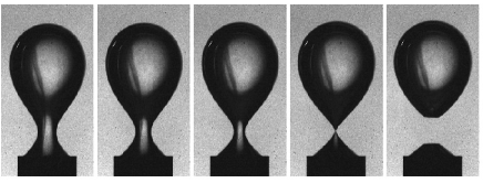
Figure 9: The pinch-off of an air bubble in water [125]. An initially smooth shape develops a localised pinch-point.

However both experiment [125] and simulation [122] show that the cylindrical solution is unstable; rather, the pinch region is rather localised, see Fig. 9. Therefore, it is not enough to treat the width of the cavity as a constant $L$; the width $W$ is itself a time-dependent quantity. In [122] we show that to leading order the time evolution of the integral equation (2.21rsah) can be reduced to a set of ordinary differential equations for the minimum $a_{0}$ of $a(x,t)$, as well as its curvature $a_{0}^{\prime\prime}$.

\psfrag{t'}{\Large$t^{\prime}$}\includegraphics[width=199.16928pt]{alpha1dot.eps}

Figure 10: A comparison of the exponent $\alpha$ between full numerical simulations of bubble pinch-off (solid line) and the leading order asymptotic theory (2.21rsaq) (dashed line).

Namely, the integral in (2.21rsah) is dominated by a local contribution from the pinch region. To estimate this contribution, it is sufficient to expand the profile around the minimum at $z=0$: $a(x,t)=a_{0}+(a^{\prime\prime}_{0}/2)z^{2}+O(z^{4})$. As in previous theories, the integral depends logarithmically on $a$, but the axial length scale is provided by the inverse curvature $W\equiv(2a_{0}/a^{\prime\prime}_{0})^{1/2}$. Thus evaluating (2.21rsah) at the minimum, one obtains [122] to leading order

$$\ddot{a}_{0}\ln(4W^{2}/a_{0})=\dot{a}_{0}^{2}/(2a_{0}),$$ (2.21rsak)

which is a coupled equation for $a_{0}$ and $W$. Thus, a second equation is needed to close the system, which is obtained by evaluating the the second derivative of (2.21rsah) at the pinch point:

$$\ddot{a}^{\prime\prime}_{0}\ln\left(\frac{8}{e^{3}a^{\prime\prime}_{0}}\right)-2\frac{\ddot{a}_{0}a^{\prime\prime}_{0}}{a_{0}}=\frac{\dot{a}_{0}\dot{a}_{0}^{\prime\prime}}{a_{0}}-\frac{\dot{a}_{0}^{2}a_{0}^{\prime\prime}}{2a_{0}^{2}}.$$ (2.21rsal)

The two coupled equations (2.21rsak),(2.21rsal) are most easily recast in terms of the time-dependent exponents

$$2\alpha\equiv-\partial_{\tau}a_{0}/a_{0},\quad 2\delta\equiv-\partial_{\tau}a^{\prime\prime}_{0}/a^{\prime\prime}_{0},$$ (2.21rsam)

where $\beta=\alpha-\delta$, so $\alpha,\beta$ are generalisations of the usual exponents in (1.2). The exponent $\delta$ characterises the time dependence of the aspect ratio $W$. Returning to the collapse (2.21rsai) predicted for a constant solution, one finds that $\alpha=1/2$ and $\delta=0$. In the spirit of the the previous subsection, this is the fixed point corresponding to the cylindrical solution. Now we expand the values of $\alpha$ and $\delta$ around their expected asymptotic values $1/2$ and $0$:

$$\alpha=1/2+u(\tau),\quad\delta=v(\tau).$$ (2.21rsan)

and put $w(\tau)=1/\ln(a^{\prime\prime}_{0})$.

To leading order, the resulting equations are

$$u_{\tau}=u+w/4,\quad v_{\tau}=-v-w/4,\quad w_{\tau}=2vw^{2}.$$ (2.21rsao)

The linearisation around the fixed point thus has the eigenvalues $0$ and $-1$, in addition to the eigenvalue $1$ coming from time translation. As before, the vanishing eigenvalue is the origin of the slow approach to the fixed point observed for the present problem. The derivatives $u_{\tau}$ and $v_{\tau}$ are of lower order in the first two equations of (2.21rsao), and thus to leading order $u=v$ and $v=-w/4$. Using this, the last equation of (2.21rsao) can be simplified to

$$w_{\tau}=-w^{3}/2.$$ (2.21rsap)

Equation (2.21rsap) is analogous to (2.21m), but has a degeneracy of third order, rather than second order. Equation (2.21rsap) yields, in an expansion for small $\delta$ [122],

$$\alpha=1/2+\frac{1}{4\sqrt{\tau}}+O(\tau),\quad\delta=\frac{1}{4\sqrt{\tau}}+O(\tau^{-3/2}).$$ (2.21rsaq)

Thus the exponents converge toward their asymptotic values $\alpha=\beta=1/2$ only very slowly, as illustrated in Fig. 10. This explains why typical experimental values are found in the range $\alpha\approx 0.54-0.58$ [125], and why there is a weak dependence on initial conditions [126].

3.2.2 Keller-Segel model for chemotaxis

This model describes the aggregation of microorganisms driven by chemotactic stimuli. The problem has biological meaning in 2 space dimensions. If we describe the density of individuals by $u(x,t)$ and the concentration of the chemotactic agent by $v(x,t)$, then the Keller-Segel system reads

$$u_{t} = \Delta u-\chi\nabla\cdot(u\nabla v),$$ (2.21rsara)

$$\Gamma v_{t} = \Delta v+(u-1),$$ (2.21rsarb)

where $\Gamma$ and $\chi$ are positive constants. In [13, 127] it was shown that for radially symmetric solutions of (2.21rsara),(2.21rsarb) singularities are such that to leading order $u$ blows up in the form of a delta function. The profile close to the singularity is self-similar and of the form

$$u(r,t)=\frac{1}{R^{2}(t)}U\left(\frac{r}{R(t)}\right),$$ (2.21rsaras)

where

$$R(t)=Ce^{-\frac{1}{2}\tau-\frac{\sqrt{2}}{2}\tau^{\frac{1}{2}}-\frac{1}{4}\ln\tau+\frac{1}{4}\frac{\ln\tau}{\sqrt{\tau}}}(1+o(1))$$ (2.21rsarat)

and

$$U(\xi)=\frac{8}{\chi(1+\xi^{2})}.$$ (2.21rsarau)

The result comes from a careful matched asymptotics analysis that, in our notation, amounts to introducing the time-dependent exponent

$$\gamma=-\partial_{\tau}R/R,$$ (2.21rsarav)

which has the fixed point $\gamma=1/2$. Corrections are of the form

$$\gamma=\frac{1}{2}+\frac{\alpha}{2}\left(\alpha-\alpha^{2}+1\right),$$ (2.21rsaraw)

where $\alpha$ is controlled by a third-order non-linearity, as in the bubble problem:

$$\alpha_{\tau}=-\alpha^{3}(1-\alpha+o(\alpha)).$$ (2.21rsarax)

3.3 Beyond all orders: The nonlinear Schrödinger equation

The cubic nonlinear Schrödinger equation

$$i\varphi_{t}+\Delta\varphi+\left|\varphi\right|^{2}\varphi=0\,$$ (2.21rsaray)

appears in the description of beam focusing in a nonlinear optical medium, for which the space dimension is $d=2$. Equation (2.21rsaray) belongs to the more general family of nonlinear Schrödinger equations of the form

$$i\varphi_{t}+\Delta\varphi+\left|\varphi\right|^{p}\varphi=0,$$ (2.21rsaraz)

and in any dimension $d$. Of particular interest, from the point of view of singularities, is the critical case $p=4/d$. In this case, singularities with slowly converging similarity exponents appear due to the presence of zero eigenvalues. We will describe this situation below, based on the formal construction of Zakharov [128], later proved rigorously by Galina Perelman [129]. At the moment, the explicit construction has only been given for $d=1$, that is, for the quintic Schrödinger equation. The same blow-up estimates have been shown to hold for any space dimension $d<6$ by Merle and Raphaël [130], [131], without making use of Zakharov’s [128] formal construction. Merle and Raphaël also show that the stable solutions to be described below are in fact global attractors.

In the critical case (2.21rsaraz) becomes in d=1:

$$i\varphi_{t}+\varphi_{xx}+\left|\varphi\right|^{4}\varphi=0.$$ (2.21rsarba)

This equation has explicit self-similar solutions (in the sense that rescaling $x\rightarrow\lambda x$, $t\rightarrow\lambda^{2}t$, $\varphi\rightarrow\lambda^{\frac{1}{2}}\varphi$ leaves the solutions unchanged except for the trivial phase factor $e^{-2i\mu_{0}\ln\lambda}$) of the form

$$\varphi(x,t)=e^{i\mu_{0}\tau}e^{-\frac{\xi^{2}}{8}i}\frac{1}{t^{\prime\frac{1}{4}}}\varphi_{0}(\xi),\quad\xi=x^{\prime}/t^{\prime 1/2}.$$ (2.21rsarbb)

The function $\varphi_{0}(\xi)$ solves

$$-\varphi_{0,\xi\xi}+\varphi_{0}-\left|\varphi_{0}\right|^{4}\varphi_{0}=0,$$ (2.21rsarbc)

and is given explicitly by

$$\varphi_{0}(\xi)=\frac{(3\mu_{0})^{\frac{1}{4}}}{\cosh^{\frac{1}{2}}(2\sqrt{\mu_{0}}\xi)}.$$ (2.21rsarbd)

We seek solutions of (2.21rsarba) using a generalisation of (2.21rsarbb), which allow for a variation of the phase factors, and the amplitude to be different from a power law:

$$\varphi(x,t)=e^{i\mu(t)-i\beta(t)z^{2}/4}\lambda^{\frac{1}{2}}(t)\varphi_{a}(z),$$ (2.21rsarbe)

where $z=\lambda(t)x$ and $\varphi_{a}$ satisfies

$$-\varphi_{a,\xi\xi}+\varphi_{a}-\frac{1}{4}az^{2}\varphi_{a}-\left|\varphi_{a}\right|^{4}\varphi_{a}=0.$$ (2.21rsarbf)

When $h$ $(=\sqrt{a})$ is constant, (2.21rsarbe) is a solution of (2.21rsarba) if $(\mu,\lambda,\beta)$ satisfy

$$\mu_{t} = \lambda^{2}$$ (2.21rsarbga)

$$\lambda^{-3}\lambda_{t} = \beta$$ (2.21rsarbgb)

$$\beta_{t}+\lambda^{2}\beta^{2} = \lambda^{2}h^{2}.$$ (2.21rsarbgc)

Notice that the equation for $\mu$ is uncoupled, so we only need to solve the equations for $(\lambda,\beta)$ simultaneously and then integrate the equation for $\mu$. It is interesting for the following that, in addition to the solutions for constant $a$, one can let $a$ vary slowly in time. The resulting system for $(\lambda,\beta,h)$ is

$$\lambda^{-3}\lambda_{t} = \beta$$ (2.21rsarbgbha)

$$\beta_{t}+\lambda^{2}\beta^{2} = \lambda^{2}h^{2}$$ (2.21rsarbgbhb)

$$h_{t} = -c\lambda^{2}e^{-S_{0}/h}/h.$$ (2.21rsarbgbhc)

Note the appearance of the factor $e^{-S_{0}/h}$ in the last equation, which comes from a semiclassical limit of a linear Schrödinger equation with appropriate potential (see [129]), and

$$S_{0}=\int_{0}^{2}\sqrt{1-s^{2}/4}ds=\frac{\pi}{2}.$$ (2.21rsarbgbhbi)

$S_{0}$ is an It follows from the presence of this factor that the non-linearity is beyond all orders, smaller than any given power, in contrast to the examples given above.

As in section 3.2.1, we rewrite the equations in terms of similarity exponents,

$$\alpha=-\frac{\lambda_{\tau}}{\lambda},\ \gamma=-\frac{\beta_{\tau}}{\beta},\ \delta=-\frac{h_{\tau}}{h}$$ (2.21rsarbgbhbj)

to obtain the system:

$$\alpha_{\tau} = -(1+2\alpha+\gamma)\alpha$$ (2.21rsarbgbhbka)

$$\gamma_{\tau} = (1+2\alpha+\gamma)\alpha-(\gamma+\alpha)(1+2\alpha+2\delta-\gamma)$$ (2.21rsarbgbhbkb)

$$\delta_{\tau} = (-1-2\alpha+2\delta)\delta-\delta^{2}\frac{S_{0}}{h}$$ (2.21rsarbgbhbkc)

$$h_{\tau} = -\delta h.$$ (2.21rsarbgbhbkd)

The advantage of this formulation is that the exponents have fixed points. There are two families of equilibrium points for (2.21rsarbgbhbka)-(2.21rsarbgbhbkd):

1. $\alpha=-\frac{1}{2},\ \gamma=0\ ,\delta=0,\ h$ arbitrary positive or zero.

2. $\alpha=-1,\ \gamma=1\ ,\delta=0,\ h$ arbitrary positive or zero.

We first investigate case (1) by writing

$$\alpha=-\frac{1}{2}+\alpha_{1},\ \gamma=\gamma_{1},\ \delta=\delta_{1},\ h=h_{1}.$$ (2.21rsarbgbhbkbl)

The final fixed point corresponding to the singularity is going to be $\alpha_{1}=\gamma_{1}=\delta_{1}=h_{1}=0$. However, there are also equilibrium points for any $h>0$, in which case the linearisation reads:

$$\alpha_{1,\tau} = \alpha_{1}+\frac{1}{2}\gamma_{1}$$ (2.21rsarbgbhbkbma)

$$\gamma_{1,\tau} = -\gamma_{1}+\delta_{1}$$ (2.21rsarbgbhbkbmb)

$$\delta_{1,\tau} = 2\delta_{1}^{2}-2\alpha_{1}\delta_{1}-\delta_{1}^{2}\frac{S_{0}}{h}.$$ (2.21rsarbgbhbkbmc)

This system has the matrix

$$A=\left(\begin{array}[]{ccc}1&\frac{1}{2}&0\\ 0&-1&1\\ 0&0&0\end{array}\right),$$

whose eigenvalues are: $1,0$, and $-1$. The vanishing eigenvalue corresponds to the line of equilibrium points for $h>0$, the positive eigenvalue to the direction of instability generated by a change in blow-up time. The eigenvector corresponding to the negative eigenvalue gives the direction of the stable manifold.

At the point $h=0$, there is an additional vanishing eigenvalue, and the equations become:

$$\alpha_{1,\tau^{\prime}} = (\alpha_{1}+\frac{1}{2}\gamma_{1})h_{1}$$ (2.21rsarbgbhbkbmbna)

$$\gamma_{1,\tau^{\prime}} = (-\gamma_{1}+\delta_{1})h_{1}$$ (2.21rsarbgbhbkbmbnb)

$$\delta_{1,\tau^{\prime}} = (2\delta_{1}^{2}-2\alpha_{1}\delta_{1})h_{1}-\delta_{1}^{2}S_{0}$$ (2.21rsarbgbhbkbmbnc)

$$h_{1,\tau^{\prime}} = -\delta_{1}h_{1}^{2},$$ (2.21rsarbgbhbkbmbnd)

where $d\tau^{\prime}=d\tau/h_{1}$. The first two equations reduce to leading order to $\gamma_{1}=\delta_{1}h_{1}$ and $\alpha_{1}=-\delta_{1}h_{1}^{2}/2$, while the last two equations reduce to the nonlinear system:

$$\delta_{1,\tau^{\prime}}=-\delta_{1}^{2}S_{0},\quad h_{1,\tau^{\prime}}=-\delta_{1}h_{1}^{2},\quad\tau_{\tau^{\prime}}=h_{1}.$$ (2.21rsarbgbhbkbmbnbo)

In the original $\tau$-variable, the dynamical system is

$$\delta_{1,\tau}=-\delta_{1}^{2}S_{0}/h_{1}\quad h_{1,\tau^{\prime}}=-\delta_{1}h_{1},$$ (2.21rsarbgbhbkbmbnbp)

which controls the approach to the fixed point. The system (2.21rsarbgbhbkbmbnbp) is two-dimensional, corresponding to the two vanishing eigenvalues.

Integrating the first equation of (2.21rsarbgbhbkbmbnbo) one gets $\delta_{1}\sim 1/(S_{0}\tau^{\prime})$, and thus using the second equation $h_{1}\sim S_{0}/\ln\tau^{\prime}$. From the last equation one obtains to leading order $\tau^{\prime}\sim\tau\ln\tau/S_{0}$, so that

$$h_{1}\sim\frac{S_{0}}{\ln\tau}\ ,\ \delta_{1}\sim\frac{1}{\tau\ln\tau}.$$ (2.21rsarbgbhbkbmbnbq)

Thus we can conclude that

$$\alpha(\tau)\simeq\frac{1}{2}-\frac{1}{2\tau\ln\tau},\quad\gamma(\tau)\simeq\frac{1}{\tau\ln\tau},\quad\delta(\tau)\simeq\frac{1}{\tau\ln\tau}.$$ (2.21rsarbgbhbkbmbnbr)

In this fashion, one can construct a singular solution such that

$$\varphi(x,t)=e^{-i\tau\ln\tau-i\frac{1}{t^{\prime}}x^{2}/4}\frac{(\ln\tau)^{\frac{1}{4}}}{t^{\prime\frac{1}{4}}}\varphi_{h^{2}\tau}\left(\frac{(\ln\tau)^{\frac{1}{2}}}{t^{\prime\frac{1}{2}}}x\right)$$

$$\sim e^{-i\tau\ln\tau}\frac{(\ln\tau)^{\frac{1}{4}}}{t^{\prime\frac{1}{4}}}\varphi_{0}\left(\frac{(\ln\tau)^{\frac{1}{2}}}{t^{\prime\frac{1}{2}}}x\right)$$ (2.21rsarbgbhbkbmbnbs)

Note the remarkable smallness of this correction to the “natural” scaling exponent of $t^{\prime 1/4}$, which enters only as the logarithm of logarithmic time $\tau$.

The fixed points (2) can be analysed in a similar fashion. The linearisation leads to

$$\alpha_{1,\tau} = 2\alpha_{1}+\gamma_{1}$$ (2.21rsarbgbhbkbmbnbta)

$$\gamma_{1,\tau} = \gamma_{1}$$ (2.21rsarbgbhbkbmbnbtb)

$$\delta_{1,\tau} = \delta_{1}.$$ (2.21rsarbgbhbkbmbnbtc)

All eigenvalues are positive, so one cannot expect these equilibrium points to be stable.

One may also consider the blow-up of vortex solutions to both critical and supercritical solutions to nonlinear Schrödinger equation in 2D. These are a subset of the general solutions to NLSE that present a phase singularity at a given point. The singularities appear in the form of collapse of rings at that point. Both the existence of such solutions and their stability have been considered recently in [132, 133].

3.3.1 Other nonlinear dispersive equations

The nonlinear Schrödinger equation belongs to the broader class of nonlinear dispersive equations, for which many questions concerning existence and qualitative properties of singular solutions are still open. Nevertheless, there have been recent developments that we describe next.

The Korteweg-de Vries (KdV) equation

$$u_{t}+(u_{xx}+u^{2})_{x}=0$$ (2.21rsarbgbhbkbmbnbtbu)

describes the propagation of waves with large wave-length in a dispersive medium. For example, this is the case of water waves in the shallow water approximation, where $u$ represents the height of the wave. In the case of an arbitrary exponent of the nonlinearity, (2.21rsarbgbhbkbmbnbtbu) becomes the generalised Korteweg de Vries equation:

$$u_{t}+(u_{xx}+u^{p})_{x}=0\ ,\ p>1.$$ (2.21rsarbgbhbkbmbnbtbv)

Based on numerical simulations, [134] conjectured the existence of singular solutions of (2.21rsarbgbhbkbmbnbtbv) with type-I self-similarity if $p\geq 5$. In [135], [136] it was shown that in the critical case $p=5$ solutions may blow-up both in finite and in infinite time. Lower bounds on the blow-up rate were obtained, but they exclude blow-up in the self-similar manner proposed by [134].

The Camassa-Holm equation

$$u_{t}-u_{xxt}+3u_{x}u=2u_{x}u_{xx}+u_{xxx}u$$ (2.21rsarbgbhbkbmbnbtbw)

also represents unidirectional propagation of surface waves on a shallow layer of water. It’s main advantage with respect to KdV is the existence of singularities representing breaking waves [137]. The structure of these singularities in terms of similarity variables has not been addressed to our knowledge.

4 Travelling wave

The pinching of a liquid thread in the presence of an external fluid is described by the Stokes equation [138]. For simplicity, we consider the case that the viscosity $\eta$ of the fluid in the drop and that of the external fluid are the same. An experimental photograph of this situation is shown in Fig. 1. To further simplify the problem, we make the assumption (the full problem is completely analogous) that the fluid thread is slender. Then the equations given in [5] simplify to

$$h_{t}=-v_{x}h/2-vh_{x},$$ (2.21rsarbgbhbkbmbnbta)

where

$$v=\frac{1}{4}\int_{x_{-}}^{x_{+}}\left(\frac{h^{2}(y)}{\sqrt{h^{2}(y)+(x-y)^{2}}}\right)_{y}\kappa\;dy,$$ (2.21rsarbgbhbkbmbnbtb)

and the mean curvature is given by (2.2). Here we have written the velocity in units of the capillary speed $v_{\eta}=\gamma/\eta$. The limits of integration $x_{-}$ and $x_{+}$ are for example the positions of the plates which hold a liquid bridge [139].

Dimensionally, one would once more expect a local solution of the form

$$h(x,t)=t^{\prime}H\left(\frac{x^{\prime}}{t^{\prime}}\right),$$

and $H(\xi)$ has to be a linear function at infinity to match to a time-independent outer solution. In similarity variables, (2.21rsarbgbhbkbmbnbtb) has the form

$$V(\xi)=\frac{1}{4}\int^{x_{b/t^{\prime}}}_{-x_{b}/t^{\prime}}\left(\frac{H^{2}(\eta)}{\sqrt{H^{2}(\eta)+(\xi-\eta)^{2}}})\right)_{\eta}\kappa\;d\eta.$$ (2.21rsarbgbhbkbmbnbtc)

We have chosen $x_{b}$ as a real-space variable close to the pinch-point, such that the similarity description is valid in $[-x_{b},x_{b}]$. But if $H$ is linear, the integral in (2.21rsarbgbhbkbmbnbtc) diverges like $b\ln t^{\prime}$, where

$$b=-\frac{1}{4}\left[\frac{H_{+}}{1+H_{+}^{2}}+\frac{H_{-}}{1+H_{-}^{2}}\right].$$ (2.21rsarbgbhbkbmbnbtd)

Here $H_{+}$ and $H_{-}$ are the slopes of the similarity profile at $\pm\infty$. But this means that a simple “fixed point” solution (4) is impossible.

However by subtracting the singularity as $t^{\prime}\rightarrow 0$, one can define a self-similar velocity profile according to

$$V^{\rm{(fin)}}(\xi)=\lim_{\Lambda\to\infty}\frac{1}{4}\int^{\Lambda}_{-\Lambda}\left(\frac{H^{2}(\eta)}{\sqrt{H^{2}(\eta)+(\xi-\eta)^{2}}}\right)_{\eta}\kappa\;d\eta+b\ln\Lambda,$$ (2.21rsarbgbhbkbmbnbte)

where now

$$V(\xi)=V^{\rm{(fin)}}(\xi)-b\tau,$$ (2.21rsarbgbhbkbmbnbtf)

and an arbitrary constant has been absorbed into $V^{\rm{(fin)}}$. In terms of $V^{\rm{(fin)}}$, and putting

$$h(x,t)=t^{\prime}H\left(\xi,\tau\right),$$

the dynamical system for $H$ becomes

$$H_{\tau}=H-\left(\xi+V^{\rm(fin)}\right)H_{\xi}-HV^{\rm(fin)}_{\xi}/2+b\tau H_{\xi}.$$

This equation has a solution in the form of a travelling wave:

$$H(\xi,\tau)=\overline{H}(\zeta),\quad V^{\rm(fin)}(\xi,\tau)=\overline{V}(\zeta),\quad\mbox{where}\quad\zeta=\xi-b\tau.$$ (2.21rsarbgbhbkbmbnbtg)

The profiles $\overline{H},\overline{V}$ of the travelling wave obey the equation

$$\overline{H}-(\zeta+\overline{V})\overline{H}_{\zeta}=\overline{H}\;\overline{V}_{\zeta}/2.$$

The numerical solution of the integro-differential equation (4) gives

$$h_{\min}=a_{\rm{out}}v_{\eta}t^{\prime},\quad\mbox{where}\quad a_{\rm{out}}=0.033.$$ (2.21rsarbgbhbkbmbnbth)

The slope of the solution away from the pinch-point are given by

$$H_{+}=6.6\quad\mbox{and}\quad H_{-}=-0.074,$$ (2.21rsarbgbhbkbmbnbti)

which means the solution is very asymmetric, as confirmed directly from Fig. 1. These results are reasonably close to the exact result, based on a full solution of the Stokes equation [5]; in particular, the normalised minimum radius is $a_{\rm{out}}=0.0335$ for the full problem.

5 Limit cycles

An example for this kind of blow-up was introduced into the literature in [15] in the context of cosmology. There is considerable numerical evidence [140] that discrete self-similarity occurs at the mass threshold for the formation of a black hole. The same type of self-similarity has also been proposed for singularities of the Euler equation [141, 67], the porous medium equation driven by buoyancy [141], and for a variety of other phenomena [142]. A reformulation of the original cosmological problem leads to the following system:

$$f_{x}=\frac{(a^{2}-1)f}{x},$$ (2.21rsarbgbhbkbmbnbtaa)

$$(a^{-2})_{x}=\frac{1-(1+U^{2}+V^{2})/a^{2}}{x},$$ (2.21rsarbgbhbkbmbnbtab)

$$(a^{-2})_{t}=\left[\frac{(f+x)U^{2}-(f-x)V^{2}}{x}+1\right]/a^{2}-1,$$ (2.21rsarbgbhbkbmbnbtac)

$$U_{x}=\frac{f[(1-a^{2})U+V]-xU_{t}}{x(f+x)},$$ (2.21rsarbgbhbkbmbnbtad)

$$V_{x}=\frac{f[(1-a^{2})U+V]+xV_{t}}{x(f-x)}.$$ (2.21rsarbgbhbkbmbnbtae)

In [16], the self-similar description corresponding to the system (2.21rsarbgbhbkbmbnbtaa)-(2.21rsarbgbhbkbmbnbtae) was solved using formal asymptotics and numerical shooting procedures. This leads to the solutions observed in [15]. We now propose another system, which shares some of the structure of (2.21rsarbgbhbkbmbnbtaa)-(2.21rsarbgbhbkbmbnbtae), but which we are able to solve analytically:

$$u_{t}(x,t)=2f(x,t)v(x,t),$$ (2.21rsarbgbhbkbmbnbtaba)

$$v_{t}(x,t)=-2f(x,t)u(x,t),$$ (2.21rsarbgbhbkbmbnbtabb)

$$f_{t}(x,t)=f^{2}(x,t).$$ (2.21rsarbgbhbkbmbnbtabc)

The system (2.21rsarbgbhbkbmbnbtaba)-(2.21rsarbgbhbkbmbnbtabc) is driven by the simplest type of blow-up equation (2.21rsarbgbhbkbmbnbtabc), and can be solved using characteristics. However, in the spirit of this review, we transform to similarity variables according to:

$$u=U(\xi,\tau)$$ (2.21rsarbgbhbkbmbnbtabca)

$$v=V(\xi,\tau)$$ (2.21rsarbgbhbkbmbnbtabcb)

$$f=t^{\prime-1}F(\xi,\tau)$$ (2.21rsarbgbhbkbmbnbtabcc)

It is seen directly from (2.21rsarbgbhbkbmbnbtabc) that $f$ first blows up at a local maximum $f_{max}>0$. Near a maximum, the horizontal scale is the square root of the vertical scale $t^{\prime}$, and thus we must have $\xi=x^{\prime}/t^{\prime 1/2}$. With that, the similarity equations become

$$U_{\tau}=-\xi U_{\xi}/2+FV$$ (2.21rsarbgbhbkbmbnbtabcda)

$$V_{\tau}=-\xi V_{\xi}/2-FU$$ (2.21rsarbgbhbkbmbnbtabcdb)

$$F_{\tau}=-F-\xi F_{\xi}/2+F^{2}.$$ (2.21rsarbgbhbkbmbnbtabcdc)

The fixed point solution of the last equation is

$$F=\frac{1}{1+c\xi^{2}},$$ (2.21rsarbgbhbkbmbnbtabcde)

where $c>0$ is a constant. The equations for $U,V$ are solved by the ansatz

$$U=U_{0}\sin\left(C(\xi)+\tau\right),\quad V=U_{0}\cos\left(C(\xi)+\tau\right),\quad$$ (2.21rsarbgbhbkbmbnbtabcdf)

and for the function $C(\xi)$ one finds

$$\xi C^{\prime}(\xi)/2=F-1,$$ (2.21rsarbgbhbkbmbnbtabcdg)

with solution $C(\xi)=-\ln(1+c\xi^{2})$. Thus (a single component of) the singular solution is indeed of the general form

$$U=\psi(\phi(\xi)+\tau),$$ (2.21rsarbgbhbkbmbnbtabcdh)

where $\psi$ is periodic in $\tau$. This is a particularly simple version of discretely self-similar behaviour, i.e. when $T$ is the period of $\psi$, the same self-similar picture is obtained for $\tau=\tau_{0}+nT$.

6 Strange attractors and exotic behaviour

In connection to limit cycles and in the context of singularities in relativity, a few interesting situations have been found numerically quite recently. One of them is the existence of Hopf bifurcations where a self-similar solution (a stable fixed point) is transformed into a discrete self-similar solution (limit cycle) as a certain parameter varies (see [143]). Other kinds of bifurcations, for example of the Shilnikov type, are found as well [144]. Before coming to simple explicit examples, we mention that possible complex dynamics in $\tau$ has long been suggested for simplified versions of the inviscid Euler equations [145, 146, 141]. For a critical discussion of this work, see [147, 81].

The problems considered in these papers were the 2D axisymmetric Euler equations with swirl, which produces a centripetal force. In the limit that the rotation is confined to a small annulus, the direction of acceleration is locally uniform, and the equation reduces to that of 2D Boussinesq convection, where the centripetal force is replaced by a “gravity” force. Another related model is 2D porous medium convection, for which the equation reads

$$\frac{\partial T}{\partial t}+\left(T{\bf e}_{y}-\nabla\phi\right)\cdot\nabla T=0,$$ (2.21rsarbgbhbkbmbnbtabcda)

where ${\bf v}=T{\bf e}_{y}-\nabla\phi$ plays the role of the velocity field and $T$ is the temperature. The potential $\phi$ follows from the constraint of incompressibility, which gives $\triangle\phi=T_{y}$. Simulations provide evidence of a self-similar dynamics of the form [141]

$$T=t^{\prime\eta}M({\bf x}^{\prime}/t^{\prime 1+\eta},\tau),$$ (2.21rsarbgbhbkbmbnbtabcdb)

where $\eta$ is approximately 0.1 and $M$ is a function that is slowly varying with $\tau$.

Depending on the model, both periodic behaviour as well as more complicated, chaotic motion has been observed in numerical simulations. Oscillations of temperature in $\tau$ are motivated by the observation that a sharp, curved interface (i.e. the transition region between a rising “bubble” of hot fluid and its surroundings) becomes unstable and rolls up. However, owing to incompressibility, the sheet is also stretched, which stabilises the interface, leading to an eventual decrease in gradients. Locality suggests that this process could repeat itself periodically on smaller and smaller scales [141]. However, simulations of the Euler equation have also shown examples of a more complicated dependence on $\tau$, which might be chaotic behaviour [145]. We also mention that corresponding chaotic behaviour has been proposed for the description of spin glasses in the theory of critical phenomena [148]. We now give some explicit examples of chaos in the description of a singularity.

In section 3.1.1 we treated a system of an infinite number of ordinary differential equations for the coefficients of the expansion of an arbitrary perturbation to an explicit solution. Such high-dimensional systems in principle allow for a rich variety of dynamical behaviours, including those found in classical finite dimensional dynamical systems, such as chaos. Consider for instance an equation for the perturbation $g$ (the analogue of (2.21g)) of the form

$$g_{\tau}=\mathit{L}g+F(g,g),$$ (2.21rsarbgbhbkbmbnbtabcdc)

where $\mathit{L}g$ is a linear operator. Assuming an appropriate non-linear structure for the function $F$, an arbitrary nonlinear (chaotic) dynamics can be added.

To give an explicit example of a system of PDE’s exhibiting chaotic dynamics, consider the structure of the example given in section 5. It can be generalised to produce any low-dimensional dynamics near the singularity, as follows by considering the system (2.21rsarbgbhbkbmbnbtaba)-(2.21rsarbgbhbkbmbnbtabc)

$$u^{(i)}_{t}(x,t)=2fF_{i}(\{u^{(i)}\}),\quad i=1,\dots,n,$$ (2.21rsarbgbhbkbmbnbtabcdda)

$$f_{t}(x,t)=f^{2}(x,t).$$ (2.21rsarbgbhbkbmbnbtabcddb)

Using the ansatz analogous to (2.21rsarbgbhbkbmbnbtabcdf):

$$u^{(i)}=U^{(i)}\left(C(\xi)+\tau,\xi\right),$$ (2.21rsarbgbhbkbmbnbtabcdde)

and choosing $C(\xi)=-\ln(1+c\xi^{2})$, one obtains the system

$$U^{(i)}_{\tau}=F_{i}\left\{U^{(i)}\right\}.$$ (2.21rsarbgbhbkbmbnbtabcddf)

To be specific, we consider $n=3$ and

$$F_{1}=\sigma(u^{(2)}-u^{(1)}),\quad F_{2}=\rho u^{(1)}-u^{(2)}-u^{(1)}u^{(3)},\quad F_{3}=u^{(1)}u^{(2)}-\beta u^{(3)},$$ (2.21rsarbgbhbkbmbnbtabcddg)

so that (2.21rsarbgbhbkbmbnbtabcddf) becomes the Lorenz system [149]. As before, for $t^{\prime}\rightarrow 0$, the variable $\tau$ goes to infinity, and near the singularity one is exploring the long-time behaviour of the dynamical system (2.21rsarbgbhbkbmbnbtabcdde). In the case of (2.21rsarbgbhbkbmbnbtabcddg), and for sufficiently large $\rho$, the resulting dynamics will be chaotic. Specifically, taking $\sigma=10$, $\rho=28$, and $\beta=8/3$, as done by Lorenz [150], the maximal Lyapunov exponent is $0.906$. The initial conditions with which (2.21rsarbgbhbkbmbnbtabcdde) is to be solved depend on $\xi$. Thus the chaotic dynamics will follow a completely different trajectory for each space point. As a result, it will be very difficult to detect self-similar behaviour of this type as such, even if data arbitrarily close to the singularity time is taken. If for example a rescaled spatial picture is observed at constant intervals of logarithmic time $\tau$, the spatial structure of the singularity will appear to be very different. However, as pointed out in [145], chaotic motion is characterised by unstable periodic orbits, for which one could search numerically.

7 Multiple singularities

The singularities described so far occur at a single point $x_{0}$ at a given time $t_{0}$. This need not be the case, but blow-up may instead occur on sets of varying complexity, including sets of finite measure. We begin with a case where singularity formation involves two different points in space.

7.1 Hele-Shaw equation

A particularly rich singularity structure is found for a special case of (2.7) in one space dimension with $n=1$. Dropping the second term on the right, which will typically be small, one arrives at

$$h_{t}+(hh_{xxx})_{x}=0.$$ (2.21rsarbgbhbkbmbnbtabcdda)

This is a simplified model for a neck of liquid of width $h$ confined between two parallel plates, a so-called Hele-Shaw cell. which is a simplified model for the free surface in a so-called Hele-Shaw cell [151]. Breakup of a fluid neck inside the cell corresponds to $h$ going to zero in finite time.

Singular solutions displaying type-I self-similarity would be of the form

$$h(x,t)=t^{\prime\alpha}H(x^{\prime}/t^{\prime(\alpha+1)/4}),$$ (2.21rsarbgbhbkbmbnbtabcddb)

but are never observed. Instead, several types of pinch solutions different from (2.21rsarbgbhbkbmbnbtabcddb) have been found for (2.21rsarbgbhbkbmbnbtabcdda) using a combination of numerics and asymptotic arguments [152, 102, 153]. On one hand, singularities exhibit type-II self-similarity. On the other hand, the simple structure (2.21rsarbgbhbkbmbnbtabcddb) is broken by the fact that the location of the pinch point is moving in space. The root for this behaviour lies in the fact that two singularities are interacting over a distance much larger than their own spatial extend. Below we report on three different kinds of singularities whose existence has been confirmed by numerical simulation of (2.21rsarbgbhbkbmbnbtabcdda).

The first kind of singularity was called the imploding singularity in [153], since it consists of two self-similar solutions which form mirror images, and which collide at the singular time. Locally, the solution can be written

$$h(x,t)=t^{\prime 6}H((x^{\prime}+at^{\prime})/t^{\prime 3}),$$ (2.21rsarbgbhbkbmbnbtabcddc)

where $-a$ is the constant speed of the singular point. Note that the scaling exponents do not agree with (2.21rsarbgbhbkbmbnbtabcddb). The reason is that the singularity is moving, so $h$ is the solution of

$$hh_{xxx}=J(t^{\prime})\equiv t^{\prime 3},$$ (2.21rsarbgbhbkbmbnbtabcddd)

where $J$ is determined by matching to an outer region. The similarity profile $H$ is a solution of the equation $HH^{\prime\prime\prime}=1$, with boundary conditions

$$H(\eta)\propto\eta^{2}/2,\;\eta\rightarrow-\infty;\quad H(\eta)\propto\sqrt{8/3}(A-\eta)^{3/2},\;\eta\rightarrow\infty.$$ (2.21rsarbgbhbkbmbnbtabcdde)

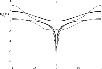
Figure 11: A simulation of (2.21rsarbgbhbkbmbnbtabcdda) with spatially periodic boundary conditions and initial condition (2.21rsarbgbhbkbmbnbtabcddf), with $w=0.02$ and $\delta=0.1$.

One might wonder whether this behaviour is generic, in the sense that it might depend on the initial conditions being exactly symmetric around the eventual point of blow up. The simulation of (2.21rsarbgbhbkbmbnbtabcdda) shown in Fig. 11 shows that this is not the case. The initial condition is

$$h(x,0)=1-(1-w)\left[\frac{3}{2}\cos\pi x-\frac{6}{10}\cos 2\pi x+\frac{1}{10}\cos 3\pi x(1+\delta\sin 2\pi x)\right],$$ (2.21rsarbgbhbkbmbnbtabcddf)

which for $\delta=0$ reduces to the symmetric initial condition considered by [153]. The type of singularity that is observed (or no singularity at all) depends on the parameter $w$. The simulation shown in Fig. 11 shows that even at finite $\delta$ (non-symmetric initial conditions) the final collapse is described by a symmetric solution.

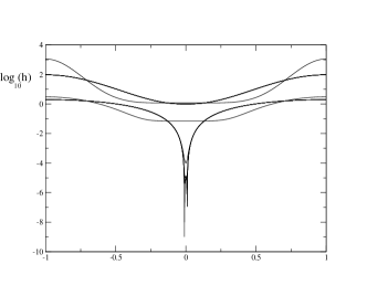
Figure 12: Same as Fig.11, but both parameters $w=0.07$ and $\delta=0.01$.

The second kind is the exploding singularity [153], since now the two self-similar solutions are moving apart, cf. Fig.12. This time even a very small asymmetry ($\delta=1/100$) makes one pinching event “win” over the other. However, this does not affect the asymptotics described briefly below. Locally, the solution can be written

$$h(x,t)=\delta^{2}(t^{\prime})H((x^{\prime}-at^{\prime})/\delta(t^{\prime})),$$ (2.21rsarbgbhbkbmbnbtabcddg)

with $\delta=t^{\prime}/ln(t^{\prime})$, which is similar to examples considered in section 3. However, an additional complication consists in the fact that the singularity is moving, so there is a coupling to the parabolic region between the two pinch-points. This matching is unaffected by the fact that in the simulation shown in Fig. 12 one side of the solution touches down first. In [153], a possible generalisation is also conjectured, which has the form

$$h(x,t)=\delta^{2}(t^{\prime})H((x^{\prime}-at^{\prime\frac{r-1}{2}})/\delta(t^{\prime})),$$ (2.21rsarbgbhbkbmbnbtabcddh)

and $\delta=t^{\prime\frac{r-1}{2}}/\ln t^{\prime}$. In principle, any value of $r$ is possible, but numerical evidence has been found for $r\approx 3$ (above) and $r\approx 5/2$ only.

Finally, a third type is the symmetric singularity of [153], which does not move. In that case, the structure of the solution is

$$h(x,t)=h_{0}(t^{\prime})H((x^{\prime}/\delta(t^{\prime})),$$ (2.21rsarbgbhbkbmbnbtabcddi)

with $h_{0}=\delta^{2}P(\ln\delta)$, where $P$ is a polynomial. The time dependence of $\delta$ is not reported. Evidently, many aspects of the exploding and of the symmetric singularity remain to be confirmed and/or to be worked out in more detail.

The most intriguing feature of the Hele-Shaw equation (2.21rsarbgbhbkbmbnbtabcdda) is that several types of stable singularities have been observed for the same equation. Within a one-parameter family of smooth initial conditions, all three types of singularities can be realized as $h\rightarrow 0$. Each type is observed over an interval of the parameter $w$. Near the boundary of the intervals, a very interesting crossover phenomenon occurs: the solution is seen to follow one type of singularity at first (the exploding singularity, say), and then crosses over to a solution of another singularity (the imploding singularity). The dynamics of each singularity can be followed numerically over many decades in $t^{\prime}$. By tuning $w$, the crossover can be made to occur at arbitrarily small values of $h$.

The switch in behaviour is driven by the slow dynamics of scaling regions exterior to (2.21rsarbgbhbkbmbnbtabcddc) or (2.21rsarbgbhbkbmbnbtabcddg). It is a signature of the very long-ranged interactions (both in real space as well as in scale), that exist in (2.21rsarbgbhbkbmbnbtabcdda). Thus an outside development can trigger a change of behaviour that is taking place on the local scale of the singularity. To mention another example, applying different boundary conditions for the pressure at the outside of the cell can change the singular behaviour completely [154]. This makes the crossover behaviour of (2.21rsarbgbhbkbmbnbtabcdda) very different from that observed for drop pinch-off (cf. (2.10),(2.11)), which is driven by a change in the dominant balance between different terms in (2.11).

7.2 Semilinear wave equation

It appears that the Hele-Shaw equation is not an isolated example, but rather is representative of a more general phenomenon. Namely, another example of a potentially complex singularity structure is the semilinear wave equation

$$u_{tt}-\Delta u=|u|^{p-1}u,\ p>1.$$ (2.21rsarbgbhbkbmbnbtabcddj)

It has trivial singular solutions of the form

$$u(x,t)=b_{0}(T-t)^{-\frac{2}{p-1}},$$ (2.21rsarbgbhbkbmbnbtabcddk)

with $b_{0}=\left[\frac{2(p+1)}{(p-1)^{2}}\right]^{\frac{1}{p-1}}$. Nevertheless, the existence of different self-similar solutions is known in a few particular cases, like the case $p\geq 7$, where $p$ is an odd integer (see [155]) or in space dimension $d=1$ (see [156]).

The character of the blow-up is controlled by the blow-up curve $T(x)$, which is the locus where the equation first blows up at a given point in space. It has been shown for $d=1$ [157] that there exists a set of characteristic points, where the blow-up curve locally coincides with the characteristics of (2.21rsarbgbhbkbmbnbtabcddj). The set of non-characteristic points $I_{0}$ is open, and $T$ is $C^{1}$ on $I_{0}$. Recently, it has been shown [158] that the blow-up at characteristic points is of type II. Even more intriguingly, it appears [158] that the structure of blow-up at these points is such that the singularity results from the collision of two peaks at the blow-up point, very similar to the observation shown in Fig. 11.

7.3 More complicated sets

In the Hele-Shaw equation of the previous subsection, different parts of the solution, characterised by different scaling laws, interacted with each other. In the generic case, however, finally blow-up only occurred at a single point in space. An example where singularities may even occur on sets of finite measure is given by reaction-diffusion equations of the family

$$u_{t}-\Delta u=u^{p}-b\left|\nabla u\right|^{q}\quad\mbox{for}\quad x\in\Omega.$$ (2.21rsarbgbhbkbmbnbtabcddl)

where $\Omega$ is any bounded, open set in dimension $d$. Depending on the values of $p>1$ and $q>1$ singularities of (2.21rsarbgbhbkbmbnbtabcddl) may be regional ($u$ blows up in subsets of $\Omega$ of finite measure), or even global (the solution blows-up in the whole domain); see for instance [159] and references therein.

Singularities may even happen in sets of fractional Hausdorff dimension, i.e., fractals. This is the case of the inviscid one-dimensional system for jet breakup (cf. [160]) and might be case of the Navier-Stokes system in three dimensions, where the dimension of the singular set at the time of first blow-up is at most $1$ (cf. [161]). This connects to the second issue we did not address here. It is the nature of the singular sets both in space and time, i.e. including possible continuation of solutions after the singularity. In some instances, existence of global in time (for all $0\leq t<\infty$) solutions to nonlinear problems can be established in a weak sense. For example, this has been achieved for systems like the Navier Stokes equations [162], reaction-diffusion equations [163], and hyperbolic systems of conservation laws [96]. Weak solutions allow for singularities to develop both in space and time. In the case of the three-dimensional Navier-Stokes system, the impossibility of singularities ”moving” in time, that is of curves $\mathbf{x}=\mathbf{\varphi}(t)$ within the singular set is well-known [161]. Hence, provided certain kinds of singularities do not persist in time, the question is how to continue the solutions after a singularity has developed.

References

References

- [1] Levine H A 1990 SIAM Review 32 262
- [2] Caflisch R C and Papanicolau G, eds 1993 Singularities in fluids, plasmas and optics (Kluwer)
- [3] Kadanoff L P 1997 Phys. Today 50(9) 11–12
- [4] Straughan B 1998 Explosive instabilities in mechanics (Springer)
- [5] Cohen I, Brenner M P, Eggers J and Nagel S R 1999 Phys. Rev. Lett. 83 1147
- [6] Eggers J 1997 Rev. Mod. Phys. 69 865–929
- [7] Moffatt H K 2000 J. Fluid Mech. 409 51
- [8] Grauer R, Marliani C and Germaschewski K 1998 Phys. Rev. Lett. 80 4177
- [9] Córdoba D, Fontelos M A, Mancho A M and Rodrigo J L 2005 PNAS 102 5949
- [10] Audoly B and Boudaoud A 2003 Phys. Rev. Letters 91 086105
- [11] Bergé L and Rasmussen J J 2002 Phys. Lett. A 304 136
- [12] Moll K D, Gaeta A L and Fibich G 2003 Phys. Rev. Lett. 90 203902
- [13] Herrero M A and Velázquez J J L 1996 Math. Ann. 306 583–623
- [14] Brenner M P, Constantin P, Kadanoff L P, Schenkel A and Venkataramani S C 1999 Nonlinearity 12 1071
- [15] Choptuik M W 1993 Phys. Rev. Lett. 70 9
- [16] Martin-Garcia J M and Gundlach C 2003 Phys. Rev. D 68 024011
- [17] Sornette D 2003 Phys. Rep. 378 1–98
- [18] Giga Y and Kohn R V 1985 Comm. Pure Appl. Math. 38 297
- [19] Giga Y and Kohn R V 1987 Indiana University Math. J. 36 1
- [20] Galaktionov V A and Vazquez J L 2004 A Stability Technique for Evolution Partial Differential Equations: A Dynamical Systems Approach (Birkhauser)
- [21] Coddington E A and Levinson N 1955 Theory of Ordinary Dierential Equations (McGraw-Hill)
- [22] Levitan B M and Sargsjan I S 1990 Sturm-Liouville and Dirac Operators (Springer)
- [23] Goldenfeld N 1993 Lectures on phase transitions and the renormalization group (Addison-Wesley)
- [24] Bricmont J, Kupiainen A and Lin G 1994 Comm. Pure Appl. Math. 47 893
- [25] Chen L, Debenedetti P G, Gear C W and Kevrekidis I G 2004 J. Non-Newtonian Fluid Mech. 120 215
- [26] Arnold V I 1984 Catastrophe Theory (Springer)
- [27] Pomeau Y, Le Berre M, Guyenne P and Grilli S 2008 Nonlinearity 21 T61–T79
- [28] Angenent S B and Aronson D G 2003 J. evol. equ. 3 137
- [29] Berry M V 2007 Proc. R. Soc. A 463 3055
- [30] Angenent S B and Velázquez J J L 1997 J. reine angew. Math. 482 15
- [31] Martin-Garcia J M and Gundlach C 2007 Living Rev. Rel. 10 5 URL http://www.livingreviews.org/lrr-2007-5
- [32] Barenblatt G I and Zel’dovich Y B 1972 Annu. Rev. Fluid Mech. 4 285–312
- [33] Sedov L I 1993 Similarity and dimensional methods in mechanics (CRC Press)
- [34] Sachdev P L 2004 Shock Waves and Explosions (Chapman and Hall)
- [35] Barenblatt G I 1996 Similarity Self-Similarity and Intermedeate Asymptotics (Cambridge)
- [36] Mizushima I, Sato T, Taniguchi S and Tsunashima Y 2000 Appl. Phys. Lett. 77 3290–3292
- [37] Nichols F A and Mullins W W 1965 J. Appl. Phys. 36 1826
- [38] Spohn H 1993 J. Phys. I (France) 3 69
- [39] Stone H A, Aziz M J and Margetis D 2005 J. Appl. Phys. 97 113535
- [40] Margetis D, Aziz M J and Stone H A 2004 Phys. Rev. Lett 69 041404
- [41] Margetis D, Fok P W, Aziz M J and Stone H A 2006 Phys. Rev. Lett. 97 096102
- [42] Eggers J 2005 ZAMM 85 400
- [43] Bernoff A J, Bertozzi A L and Witelski T P 1998 J. Stat. Phys. 93 725–776
- [44] Pugh M C 2006 Notes on blowup and long wave unstable thin film equations URL http://topo.math.auburn.edu/pub/2Olgas-proceedings/
- [45] Zhang W W and Lister J R 1999 Phys. Fluids 11 2454–2462
- [46] Witelski T P and Bernoff A J 2000 Physica D 147 155–176
- [47] Becker J and Grün G 2005 J. Phys.: Condens. Matter 17 S291–S307
- [48] Chou K S and Kwong Y C 2007 Nonlinearity 20 299–317
- [49] Eggers J and Villermaux E 2008 Rep. Progr. Phys. 71 036601
- [50] Eggers J 1993 Phys. Rev. Lett. 71 3458
- [51] Brenner M P, Lister J R and Stone H A 1996 Phys. Fluids 8 2827
- [52] Papageorgiou D T 1995 Phys. Fluids 7 1529
- [53] Eggers J 2005 Phys. Fluids 17 082106
- [54] Doshi P, Cohen I, Zhang W W, Siegel M, Howell P, Basaran O A and Nagel S R 2003 Science 302 1185
- [55] Ting L and Keller J B 1990 SIAM J. Appl. Math. 50 1533
- [56] Fontelos M A and Velázquez J J L 1999 SIAM J. Appl. Math. 59 2274
- [57] Eggers J 2000 SIAM J. Appl. Math. 60 1997
- [58] Chen Y J and Steen P H 1997 J. Fluid Mech. 341 245–267
- [59] Day R F, Hinch E J and Lister J R 1998 Phys. Rev. Lett. 80 704
- [60] Leppinen D and Lister J 2003 Phys. Fluids 15 568
- [61] Lenard P 1887 Ann. Phys. Chem. 30 209
- [62] Vaynblat D, Lister J R and Witelski T P 2001 Eur. J. Appl. Math. 12 209–232
- [63] Gibbon J D, Moore D R and Stuart J T 2003 Nonlinearity 16 1823
- [64] Necas J, Ruzicka M and Sverak V 1996 Acta Math. 176 283–294
- [65] Pelz R B 1997 Phys. Rev. E 55 1617 – 1626
- [66] Hou T Y and Li R 2008 Physica D 237 1937–1944
- [67] Pomeau Y and Sciamarella D 2005 Physica D 205 215
- [68] Goldstein S 1948 Q. J. Mech. Appl. Math. 1 43–69
- [69] Sychev V V, Ruban A I, Sychev V V and Korolev G L 1998 Asymptotic Theory of Separated Flows (Cambridge)
- [70] E W and Engquist B 1997 Comm Pure. Appl. Math. 50 1287–1293
- [71] Van Dommelen L L and Shen S F 1980 J. Comput. Phys. 38 125–140
- [72] Van Dommelen L L and Shen S F 1982 in T Cebeci, ed, Aspects of Aerodynamic Flows (Springer) pp 293–311
- [73] Caflisch R E and Sammartino M 2000 ZAMM, Z. Angew. Math. Mech 11-12 733–744
- [74] Elliott J W, Cowley S J and Smith F T 1983 Geophys. Astrophys. Fluid Dyn. 25 77–138
- [75] Cassel K W, Smith F T and Walker J D A 1996 J. Fluid Mech. 315 223–256
- [76] Saffman P G 1992 Vortex dynamics (Cambridge University Press)
- [77] Moore D W 1979 Proc. Roy. Soc. London A 365 105–119
- [78] Caflisch R E and Orellana O F 1989 SIAM J. Math. Anal. 20 293–307
- [79] de la Hoz F, Fontelos M A and Vega L 2008 J. Nonlin. Sci. 18 463–484
- [80] Kambe T 1989 Physica D 37 463
- [81] Majda A J and Bertozzi A L 2002 Vorticity and Incompressible Flow (Cambridge University Press)
- [82] Gutiérrez S, Rivas J and Vega L 2003 Comm. PDE 28 927–968
- [83] Craig W and Wayne C E 2007 Russ. Math. Surv. 62 453–473
- [84] Constantin P, Majda A and Tabak E 1994 Nonlinearity 7 1495
- [85] Chae D, Córdoba A, Córdoba D and Fontelos M A 2005 Advances in Mathematics 194 203–223
- [86] Córdoba A, Córdoba D and Fontelos M A 2005 Ann. of Math. 162 1375–1387
- [87] de la Hoz F and Fontelos M A 2008 J. Phys. A: Math. Theor. 41 185204
- [88] Moffatt H K 1963 J. Fluid Mech. 18 1–18
- [89] Carothers S D 1912 Proc. Roy. Soc. Edinburgh 23 292
- [90] Sternberg E and Koiter W T 1958 J. Appl. Mech. 25 575
- [91] Batchelor G K 1967 An introduction to Fluid Dynamics (Cambridge University Press)
- [92] Solomentsev Y, Velegol D and Anderson J L 1997 Phys. Fluids 9 1209
- [93] Griffith W C and Bleakney W 1954 Amer. J. Phys. 22 597
- [94] Alinhac S 1995 Blowup for nonlinear hyperbolic equations (Birkhäuser)
- [95] Whitham G B 1974 Linear and Nonlinear Waves (John Wiley & Sons)
- [96] Dafermos C M 2005 in Grundlehren der Mathematischen Wissenschaften vol 325 (Springer, Berlin)
- [97] Bressan A 2000 Hyperbolic Systems of Conservation Laws. The One Dimensional Cauchy Problem (Oxford University Press)
- [98] Landau L D and Lifshitz E M 1984 Fluid Mechanics (Pergamon: Oxford)
- [99] Rothert A, Richter R and Rehberg I 2003 New J. Phys. 5 59
- [100] Abramowitz M and Stegun I A 1968 Handbook of Mathematical Functions (Dover)
- [101] Burton J C and Taborek P 2007 Phys. Fluids 19 102109
- [102] Dupont T F, Goldstein R E, Kadanoff L P and Zhou S 1993 Phys. Rev. E 47 4182
- [103] Barenblatt G I 2003 Scaling (Cambridge)
- [104] Guderley G 1942 Luftfahrtforschung 19 302
- [105] Brenner M P and Witelski T P 1998 J. Stat. Phys. 93 863
- [106] Chavanis P H and Sire C 2004 Phys. Rev. E 69 016116
- [107] Lacaze R, Lallemand P, Pomeau Y and Rica S 2001 Physica D 152 779
- [108] Josserand C, Pomeau Y and Rica S 2006 J. Low Temp. Phys. 145 213
- [109] Filippas S and Kohn R V 1992 Comm. Pure Appl. Math. 45 821–869
- [110] Velázquez J J L, Galaktionov V A and Herrero M A 1992 Comput. Math. Math. Phys. 31 46–55
- [111] Ishiguro R, Graner F, Rolley E, Balibar S and Eggers J 2007 Phys. Rev. E 75 041606
- [112] Ishiguro R, Graner F, Rolley E and Balibar S 2004 Phys. Rev. Lett. 93 235301
- [113] Altschuler S, Angenent S and Giga Y 1995 J. Geom. Anal. 5 293
- [114] Huisken G 1993 Proc. of Symposia in Pure Math. 54 175–191
- [115] Hamilton R S 1982 Jour. Diff. Geom. 17 255–306
- [116] Perelman G 2003 Ricci flow with surgery on three-manifolds URL http://arxiv.org/abs/math.DG/0303109
- [117] Angenent S and Knopf D 2007 Comm. Anal. Geom. 15 773–844
- [118] Herrero M A and Velázquez J J L 1993 Ann. Inst. Henri Poincaré, Anal. Non Linéaire 10 131–189
- [119] Merle F and Zaag H 1998 Comm. Pure Appl. Math. 51 139–196
- [120] Galaktionov V A and Vázquez J L 2002 Discrete and Continuous dynamical systems 8 399–433
- [121] Vazquez J L 2006 Smoothing and Decay Estimates for Nonlinear Diffusion Equations. Equations of Porous Medium Type (Oxford University Press)
- [122] Eggers J, Fontelos M A, Leppinen D and Snoeijer J H 2007 Phys. Rev. Lett. 98 094502
- [123] Longuet-Higgins M S, Kerman B R and Lunde K 1991 J. Fluid Mech. 230 365
- [124] Og̃uz H N and Prosperetti A 1993 J. Fluid Mech. 257 111
- [125] Thoroddsen S T, Etoh E G and Takeara K 2007 Phys. Fluids 19 042101
- [126] Bergmann R, van der Meer D, Stijnman M, Sandtke M, Prosperetti A and Lohse D 2006 Phys. Rev. Lett. 96 154505
- [127] Herrero M A and Velázquez J J L 1996 J. Math. Biol. 35 177–194
- [128] Dyachenko S, Newell A C, Pushkarev A and Zakharov V I 1992 Physica D 57 96–160
- [129] Perelman G 2001 Ann. Henri Poincaré 2 605–673
- [130] Merle F and Raphaël P 2004 Invent. Math. 156 565–672
- [131] Merle F and Raphaël P 2006 J. Amer. Math. Soc. 19 37–90
- [132] Fibich G, Gavish N and Wang X 2007 Physica D 231 55–86
- [133] Fibich G and Gavish N 2008 Physica D 237 2696–2730
- [134] Bona J L, Dougalis V A, Karakashian O A and McKinney W R 1995 Philos. Trans. Roy. Soc. London Ser. A 351 107–164
- [135] Martel Y and Merle F 2002 Ann. Math. 155 235–280
- [136] Martel Y and Merle F 2002 J. Amer. Math. 15 617–664
- [137] Constantin A and Escher J 1998 Acta Math. 181 229–243
- [138] Lister J R and Stone H A 1998 Phys. Fluids 10 2758
- [139] Plateau J A F 1843 Acad. Sci. Bruxelles Mem. 16 3
- [140] Gundlach C 2003 Phys. Rep. 376 339–405
- [141] Pumir A, Shraiman B I and Siggia E D 1992 Phys. Rev. A 45 R5351
- [142] Sornette D 1998 Phys. Rep. 297 239–270
- [143] Hirschmann E W and Eardley D M 1997 Phys. Rev. D 56 4696–4705
- [144] Aichelburg P C, Bizon P and Tabor Z 2006 Class. Quant. Grav. 23 S299–S306
- [145] Pumir A and Siggia E D 1992 Phys. Fluids A 4 1472
- [146] Pumir A and Siggia E D 1992 Phys. Rev. Lett. 68 1511
- [147] E W and Shu C W 1994 Phys. Fluids 6 49
- [148] McKay S R, Berker A N and Kirkpatrick S 1982 Phys. Rev. Lett. 48 767
- [149] Strogatz S H 1994 Nonlinear Dynamics and Chaos (Westview Press)
- [150] Lorenz E N 1963 J. Atmos. Sci. 20 130
- [151] Almgren R 1996 Phys. Fluids 8 344
- [152] Constantin P, Dupont T F, Goldstein R E, Kadanoff L P, Shelley M J and Zhou S 1993 Phys. Rev. E 47 4169
- [153] Almgren R, Bertozzi A L and Brenner M P 1996 Phys. Fluids 8 1356
- [154] Bertozzi A L, Brenner M P, Dupont T F and Kadanoff L P 1994 in L Sirovich, ed, Applied Mathematics Series Vol 100 (Springer: New York) p 115
- [155] Bizón P, Maison D and Wasserman A 2007 Nonlinearity 20 2061–2074
- [156] Merle F and Zaag H 2007 J. Funct. Anal. 253 43–121
- [157] Merle F and Zaag H 2008 Comm. Math. Phys. 282 55
- [158] Merle F and Zaag H 2008 Existence and characterization of characteristic points for a semilinear wave equation in one space dimension URL http://arxiv.org/math/08114068
- [159] Souplet P 2001 Electron. J. Diff. Eqns. 2001-20 1–19
- [160] Fontelos M A and Velázquez J J L 2000 European J. Appl. Math. 11 29
- [161] Caffarelli L, Kohn R and Nirenberg L 1982 Comm. Pur. Appl. Math. 35 771–831
- [162] Constantin P and Foias C 1994 Navier-Stokes equations (University of Chicago Press)
- [163] Smoller J 1989 Shock waves and reaction-diffusion equations (Springer)