B2 0902+34: A COLLAPSING PROTOGIANT ELLIPTICAL GALAXY AT z=3.4

Abstract

We have used the visible integral-field replicable unit spectrograph prototype (VIRUS-P), a new integral field spectrograph, to study the spatially and spectrally resolved Lyman-$\alpha$ emission line structure in the radio galaxy B2 0902+34 at $z=3.4$. We observe a halo of Lyman-$\alpha$ emission with a velocity dispersion of $\approx$250 km s^-1 extending to a radius of 50 kpc. A second feature is revealed in a spatially resolved region where the line profile shows blueshifted structure. This may be viewed as either HI absorption at $\approx$-450 km s^-1 or secondary emission at $\approx$-900 km s^-1 from the primary peak. B2 0902+34 is also the only high redshift radio galaxy with a detection of 21 cm absorption. Our new data, in combination with the 21 cm absorption, suggest two important and unexplained discrepancies. First, nowhere in the line profiles of the Lyman-$\alpha$ halo is the 21 cm absorber population evident. Second, the 21 cm absorption redshift is higher than the Lyman-$\alpha$ emission redshift. In an effort to explain these two traits, we have undertaken the first three dimensional Monte Carlo simulations of resonant scattering in radio galaxies. We have created a simple model with two photoionized cones embedded in a halo of neutral hydrogen. Lyman-$\alpha$ photons propagate from these cones through the optically thick HI halo until reaching the virial radius. Though simple, the model produces the features in the Lyman-$\alpha$ data and predicts the 21 cm properties. To reach agreement between this model and the data, global infall of the HI is strictly necessary. The amount of gas necessary to match the model and data is surprisingly high, $\geq 10^{12}M_{\odot}$, an order of magnitude larger than the stellar mass. The collapsing structure and large gas mass lead us to interpret B2 0902+34 as a protogiant elliptical galaxy. This interpretation is a falsifiable alternative to the presence of extended HI shells ejected through feedback events such as starburst superwinds. An understanding of these gas features and a classification of this system’s evolutionary state give unique observational evidence to the formation events in massive galaxies.

1 Introduction

Progress in understanding high redshift radio galaxies (HzRGs, where we arbitrarily consider high to mean z$\gtrapprox$2) will advance our picture of both massive galaxy formation and evolution. HzRG are thought to be the progenitors of massive local cluster giant elliptical galaxies. Their radio signal allows detection over a huge range of cosmic time. We will only discuss a few revelant trends of HzRGs as extensive summaries are given by McCarthy (1993) and Miley & De Breuck (2008). Radio galaxies are found to be associated with some of the largest stellar mass galaxies at all redshifts (Lilly & Longair, 1984; Pentericci et al., 2001). The environments of massive radio galaxies have also been progressively traced to higher redshifts with radio galaxies typically residing in cluster environments at all redshifts (Longair & Seldner, 1979; Prestage & Peacock, 1988; Hill & Lilly, 1991; Carilli et al., 1997; Best, 2000). HzRGs often show extended Lyman-$\alpha$ emission up to and beyond their radio emission radii. The Lyman-$\alpha$ emission probes warm, ionized gas. Against this emission is often seen line profile structure which serves as a probe of the neutral gas through scattering and absorption. The properties of Lyman-$\alpha$ blobs (LABs) (Keel et al., 1999; Steidel et al., 2000; Palunas et al., 2004) and the gas halos of quasars (Heckman et al., 1991; Barkana & Loeb, 2003) are morphologically similar to those in HzRGs.

Cooling radiation may be an important source of extended Lyman-$\alpha$ radiation, and an indication of ongoing galaxy formation as infalling gas continues to build the galaxy’s mass (Haiman et al., 2000; Fardal et al., 2001). The most direct signature of a high redshift cooling flow is extended Lyman-$\alpha$ emission powered by the decrease in gravitational potential energy from infalling material. This is a challenging observation and interpretation as other sources of Lyman-$\alpha$ generation are usually stronger than the cooling radiation, but Nilsson et al. (2006) and Smith & Jarvis (2007) show promising cases. Low redshift cooling flows have a long history of investigation primarily through X-ray observations (e.g. Fabian, 1994), but space based observations (Kaastra et al., 2001; Peterson et al., 2001; Tamura et al., 2001) have given evidence against most cases of low redshift, strong cooling flows and diminished the importance of this mechanism for galaxy growth. Most massive galaxy growth is now thought to occur through major mergers. Li et al. (2007) show by a semi-analytic model, for example, the likely growth history of a galaxy like the SDSS quasar J1148+5251 at z=$6.42$ (Fan et al., 2003) where gas rich major mergers dominate as the source of the mass growth and a starburst phase predates a quasar phase. Observationally checking and challenging theories for the relative contributions of mergers and steady gas accretion for different galaxy types and epochs is an important goal.

In terms of evolution, AGN feedback has been proposed (Valageas & Silk, 1999) as the mechanism to produce the tight black hole/stellar mass correlation (Magorrian et al., 1998; Gebhardt et al., 2000; Ferrarese & Merritt, 2000) and the difference between the theoretical (Kaiser, 1986) and the observed (Markevitch, 1998; Arnaud & Evrard, 1999) relation between cluster temperature and X-ray luminosity. Radio galaxies in particular and their powerful jets have been invoked as candidates for causing feedback (Inoue & Sasaki, 2001; Rawlings & Jarvis, 2004; Croton et al., 2006) by depositing mechanical and thermal energy to their surroundings. A signature of outflowing gas at a velocity exceeding the halo escape speed would be an important observation of high redshift feedback.

B2 0902+34 (Lilly, 1988) is a powerful high redshift ($z\approx 3.39$) radio galaxy of moderate projected radio diameter (40 kpc, 5$\arcsec$) with a huge, diffuse Lyman-$\alpha$ halo ($\approx 100$kpc) and is one of the most thoroughly studied HzRGs. Three observations make B2 0902+34 a unique window into HzRG halos as a class. First, 21 cm absorption from HI gas against the radio source continuum has been observed at $z_{21cm}=3.3962$ (Uson et al., 1991; Briggs et al., 1993; Cody & Braun, 2003; Chandra et al., 2004), but any corresponding feature from this HI population has not shown in the Lyman-$\alpha$ emission line structure. This is the only HzRG for which 21 cm HI absorption has been repeatably measured with seven other HzRGs giving null detections (Röttgering et al., 1999; De Breuck et al., 2003). Second, Carilli (1995) used radio spectral index and polarization mapping to constrain the approaching, northern radio jet inclination to the observer to between 30$\arcdeg$ and 45$\arcdeg$. This is a particularly low inclination angle for a radio galaxy, but it does offer very different lines of sight to the two radio jets and any other structures that may follow the radio jets. Third, Villar-Martín et al. (2007a) have shown the emission line ratios in B2 0902+34 to be consistent with pure AGN photoionization through the Lyman-$\alpha$, CIV$\lambda$1549, and HeII$\lambda$1640 lines. A subsample of their HzRGs show line ratios that requires stellar photoionization. These systems would have peculiar and complicated source distributions for Lyman-$\alpha$ emission, but B2 0902+34 appears to display the relatively well understood geometry of Lyman-$\alpha$ emission powered by an AGN. Until recently, longslit spectroscopy had detected only Lyman-$\alpha$, CIV, and HeII emission lines (Martin-Mirones et al., 1995) and shown no sign of a bimodal Lyman-$\alpha$ line profile which is often seen in other HzRGs (van Ojik et al., 1997). Deeper spectroscopy and a different slit position angle revealed a spatially resolved region with a bimodal Lyman-$\alpha$ line profile (Reuland et al., 2007), with most of the emission still from a simple and quiescent line profile. We will from here forward define a quiescent Lyman-$\alpha$ line as one with $\sigma<$1000 km s^-1 to indicate emission which does not display turbulent, radio jet dominated kinematics. Reuland et al. (2007) have also reported a weak [O II]$\lambda$3727 detection in the galaxy’s center. Previous observations in deep Lyman-$\alpha$ narrowband (Reuland et al., 2003) and K broadband (Eisenhardt & Dickinson, 1992) imaging and spectroscopy of the [OIII] 5007Å line (Eales et al., 1993) have led some authors to tentatively interpret B2 0902+34 as a protogalaxy based on its flat spectral energy distribution. Reuland et al. (2003) showed a diffuse Lyman-$\alpha$ morphology with two emission peaks roughly perpendicular to the radio axis. Unlike the two other HzRGs in their sample, B2 0902+34 did not display filamentary structure in Lyman-$\alpha$.

We present the first integral field spectroscopy (IFS) data of Lyman-$\alpha$ emission in B2 0902+34. This is the fourth study of HzRGs halos using IFS after the works of Adam et al. (1997), Villar-Martín et al. (2007b), and Nesvadba et al. (2008). Le Fevre et al. (1996) and van Breukelen et al. (2005) have used IFS to search for Lyman-$\alpha$ Emitters (LAEs) around HzRGs. With knowledge of the full spatial distribution of the bimodal Lyman-$\alpha$ line profile, we create a simulation for resonant scattering of the Lyman-$\alpha$ photons through a halo of HI. We find a model that reproduces most of the important spatial and spectral properties of our IFS observation and strictly requires a collapsing structure with large HI mass. The natural explanatory power of this picture for other observations, such as the 21 cm absorption data, leads us to claim that B2 0902+34 is a protogalaxy still experiencing initial collapse.

In §2 we describe our observations. In §3 we present our new resonant scattering model and analyze the impact of our model on 21 cm measurements. We show in §4 that our data is best fit through resonant scattering against an infalling halo. In §5, we propose further discriminating observations and review. Throughout, we use a standard cosmology with H₀=71 km s^-1 Mpc^-1, $\Omega_{M}$ = 0.27, and $\Omega_{\Lambda}$ = 0.73. This gives look back times of 11.8 Gyr, angular scales of 7.5 kpc arcsec^-1, and a luminosity distance of 30 Gpc for B2 0902+34 at $z=3.4$.

2 Observations

On 2007 UT March 14 and 15 we observed B2 0902+34 with the visible integral-field replicable unit spectrograph prototype (VIRUS-P) (Hill et al., 2008) on the 2.7m Harlan J. Smith Telescope at McDonald Observatory. VIRUS-P is a spectrograph with an integral field unit (IFU) of 247 fibers in a hexagonal pattern close pack with a one third fill factor. Fed at f/3.65, the fibers have a diameter of 4.1$\arcsec$ and a 107x107 $\sq\arcsec$ field of view. Seeing was $\approx$2$\arcsec$, significantly smaller than the fiber diameter. The first night was nominally photometric, while the second was not. The instrument configuration gave us 236 working fibers spread over the field. Astrometry of the fiber positions has been calibrated to 1.0$\arcsec$ rms from a fixed, offset guide field. Observations of three offset positions (called dithers) fill in the area. We took three exposures of 1200s at each of six subdither positions. A subdither as defined here is a second dithering pattern centered on the fiber intersections of the first dither set. We use this mode to decrease the astrometric uncertainty of spatially unresolved sources, mitigate local CCD cosmetics, and subsample extended emission. The wavelength range was 3400-5680Å with a spectral resolution of 5.0Å. Wavelength calibration was done with eleven arc lamp lines of Hg and Ne yielding a $\sigma_{\lambda}=0.4$Å. Twilight flats were used to remove pixel-to-pixel variation, fiber-to-fiber variation, and the fiber illumination profile. We have used our own custom written software for all reductions. Notably, this reduction does not perform any resampling or linearization of the data. The estimates of the sky spectrum were made from neighboring objectless fibers and fit with bsplines (Dierckx, 1993) in a similar manner to optimal longslit sky subtraction methods (Kelson, 2003). We estimate a spectrally unresolved 5$\sigma$ line flux limit of $7\times 10^{-17}$ erg s^-1 cm^-2 and a surface brightness limit of 24.0 AB mag arcsec^-2 for wavelengths longer than 4000Å when under photometric conditions.

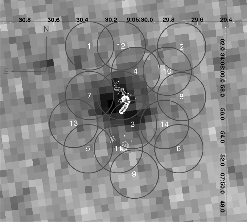
Figure 1: The fibers with detected Lyman-$\alpha$ emission are plotted over a narrowband Lyman-$\alpha$ image of the radio galaxy center. For reference, log scale contours are drawn of the 1.65 GHz image at 0.15$\arcsec$ resolution from Carilli (1995) with range 0.36-92.16 mJy/beam. Each fiber has a diameter of 4.2$\arcsec$.

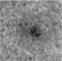
(a) Observed

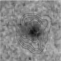
(b) Simulated, Spectral Decomposition

(c) Simulated, Origin Cone Decomposition

Figure 4: Log contours of surface brightness. Left Fits to the data. The primary and secondary peaks are respectively dark and light. Middle The simulations described in §3, where the same type of spectral decomposition as for the data between primary and secondary is performed. Right The same simulations, but now with a decomposition regardless of the spectral signature but where the dark contour follows emission from the near photoionized cone and the light contour from the rear photoionized cone. This optimistically represents a clean detangling of spectral signal that a model with more optimized parameters may accomplish.

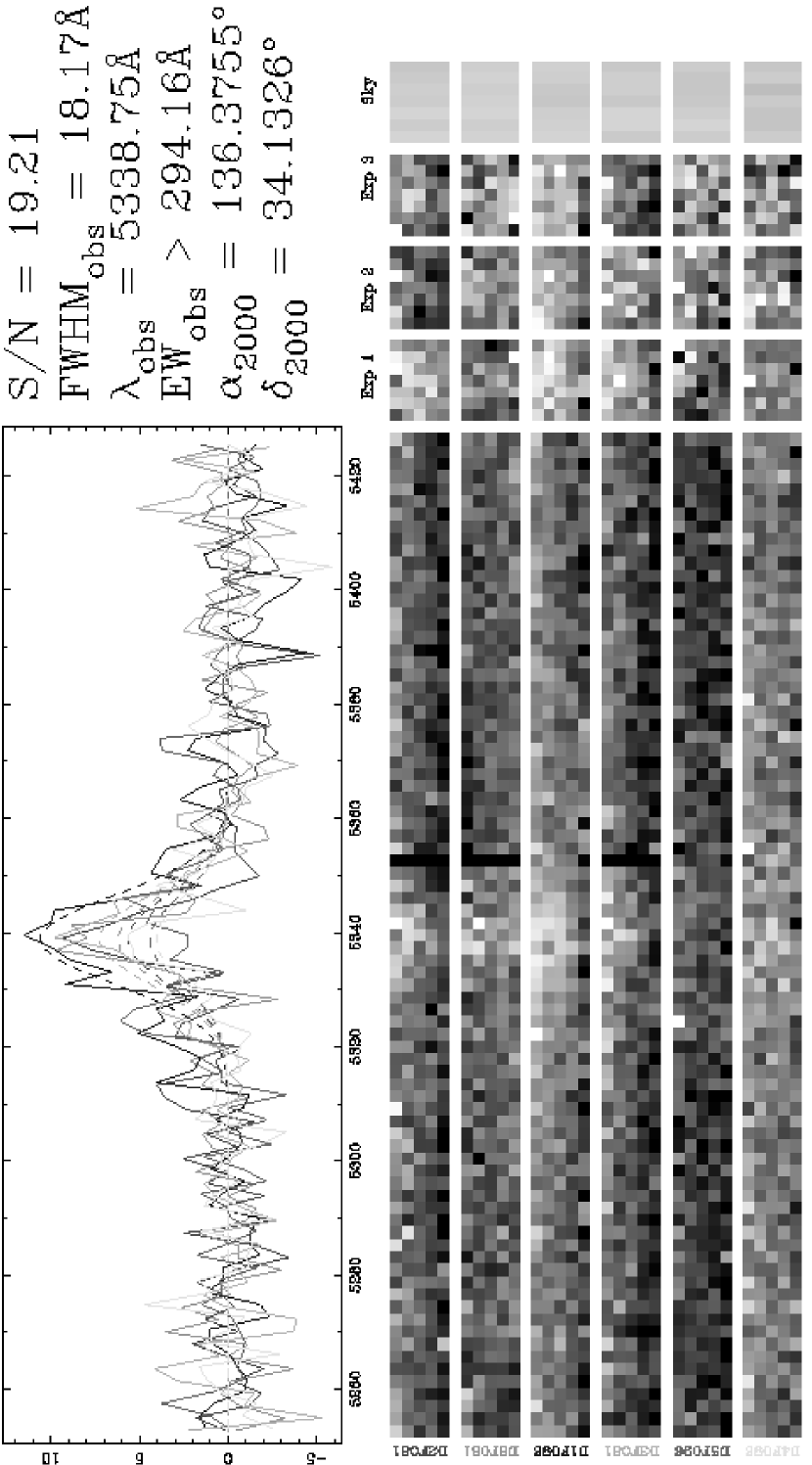
Figure 5: The joint detection of Lyman-$\alpha$ emission in a subset of the central fibers. The equivalent width limit is shown. Each row in the figure’s bottom half corresponds to the spectrum from a fiber with a unique position on sky. In the labeling of Figure 1, these fibers are numbers 4, 15, 3, 7, 14, and 11 from top to bottom.

We detected Lyman-$\alpha$ emission from the low surface brightness halo of B2 0902+34 in fifteen different fiber positions. We only include fibers that show emission above a signal-to-noise ratio of 3, calculated from the noise and counts within the full width half maximum of a single Gaussian fit. We perform Monte Carlo line fitting where 100 realizations of our data sampled from normal distributions with our estimated errors produce distributions in our fit parameters from which are extracted central values and dispersions. All uncertainty quotes are 1 sigma estimates by this method and similar to the uncertainties from the covariance matrices. All quotes of line width remove the instrument resolution in quadrature. Table 1 shows single Gaussian fits to each fiber’s spectrum. Figure 1 shows the positions of the detections against a narrowband image we have taken and the radio data of Carilli (1995). We confirm the general line profile properties reported in Reuland et al. (2007) for the region covering their slit, but our observations span the entire 2D structure. The entire halo contains an emission peak at 5339.0 $\pm$ 2.0Å with a FWHM of 600$\pm$90 km s^-1 which is well fit by a single Gaussian. This primary emission is mostly spatially symmetric and smoothly varying in brightness near the radio core emission although slightly extended toward the NE. At $\approx 15\%$ of the strength of the primary emission, a secondary emission peak can be fit as a Gaussian at 5324.5$\pm$1.7Å with a FWHM of 630$\pm$270 km s^-1. This secondary emission exists in three fibers on the SW side of the halo. Throughout this work, we will refer to any flux with a line center above 5330Å as primary emission and any flux with a line center below 5330Å as secondary emission. For the three fibers with S/N high enough for a more complex fit, we give fits in Table 2 where the fitting function consists of two independent positive Gaussians. Depending on interpretation, this feature may be due to discrete emission sites or scattering and absorption by neutral hydrogen. To aid comparison, we give fits in Table 3 with a single positive Gaussian and an absorbing Voigt function. Figure 3 shows the data and fits to select, representative spectra, and Figure 4 shows the brightness maps of the two spectrally decomposed signatures as positive Gaussians. Our data show that the longslit spectroscopy of Lilly (1988), Martin-Mirones et al. (1995), and Reuland et al. (2007) are consistent though only the latter found this secondary, bluer emission because of the different slit position angles under their observations and the different flux limits. The two dimensional spatial constraints on the secondary emission afforded by our data will be crucial to a proper interpretation. We have searched for nearby LAEs in the surrounding fibers but have found none within the field. We do not make a statistically significant detection of continuum in B2 0902+34 which places a lower limit on the rest frame equivalent width from the six brightest fibers at $>67$ Å(5 $\sigma$ continuum limit) as shown in Figure 5. We have not attempted a flux calibration due to the non-photometric conditions, so the aperture to aperture variation in surface brightness is overestimated by our data, and the flux limit between apertures is not constant.

Table 1: Individual fiber Lyman-$\alpha$ detections in B2 0902+34

Unique position	RA	Dec	Central $\lambda$	Dispersion	Normalized	S/N	$\chi^{2}$	Degrees of
number	(J2000)	(J2000)	(Å)	(Å)	Flux			Freedom
1	9:5:30.35	34:8:01.9	5339.24$\pm$7.1	11.5$\pm$9.7	0.27${}^{+0.31}_{-0.27}$	3.0	10.8	11
2	9:5:29.71	34:8:01.8	5338.96$\pm$0.9	1.1$\pm$1.5	0.19$\pm$0.07	5.2	6.4	3
3	9:5:30.05	34:7:55.1	5337.24$\pm$1.0	9.8$\pm$1.1	1.00$\pm$0.11	18.2	25.0	17
4	9:5:30.03	34:7:59.7	5338.60$\pm$0.6	3.5$\pm$0.6	0.39$\pm$0.05	9.4	1.1	5
5	9:5:30.36	34:7:53.0	5338.84$\pm$2.2	4.4$\pm$3.6	0.40$\pm$0.20	3.3	2.5	4
6	9:5:29.73	34:7:53.0	5332.51$\pm$2.8	8.8$\pm$3.2	0.33$\pm$0.11	5.3	13.1	11
7	9:5:30.35	34:7:57.6	5338.45$\pm$1.0	7.9$\pm$2.0	0.68$\pm$0.13	10.9	11.3	11
8	9:5:29.71	34:7:57.5	5339.27$\pm$1.5	4.3$\pm$2.0	0.26$\pm$0.07	3.9	7.7	5
9	9:5:30.04	34:7:50.8	5337.66$\pm$1.3	2.3$\pm$2.2	0.15$\pm$0.11	3.1	13.9	5
10	9:5:29.81	34:7:59.7	5337.92$\pm$1.0	2.5$\pm$1.0	0.20$\pm$0.05	5.1	4.4	4
11	9:5:30.15	34:7:53.0	5337.66$\pm$1.3	2.3$\pm$2.2	0.25$\pm$0.09	6.5	5.7	3
12	9:5:30.13	34:8:01.9	5336.14$\pm$5.6	6.4$\pm$5.1	0.22$\pm$0.13	4.6	16.0	7
13	9:5:30.46	34:7:55.2	5339.12$\pm$2.2	4.0$\pm$1.6	0.19$\pm$0.07	4.3	3.8	3
14	9:5:29.83	34:7:55.1	5338.03$\pm$2.9	14.1$\pm$1.9	0.68$\pm$0.16	8.6	39.8	21
15	9:5:30.13	34:7:57.6	5338.96$\pm$1.0	4.4$\pm$1.9	0.33$\pm$0.09	7.9	1.7	4

Table 2: Select regions in B2 0902+34 fit with two Gaussians

Unique position	Central $\lambda_{1}$	Dispersion1	Normalized	Central $\lambda_{2}$	Dispersion2	Normalized
number	(Å)	(Å)	Flux1	(Å)	(Å)	Flux2
2	5339.22$\pm$1.5	6.5$\pm$2.5	0.78$\pm$0.27	5323.34$\pm$7.7	3.3${}^{+5.0}_{-3.3}$	0.19${}^{+0.28}_{-0.19}$
5	5338.98$\pm$4.0	4.3$\pm$3.3	0.15$\pm$0.10	5326.97$\pm$3.2	2.8$\pm$2.7	0.14$\pm$0.09
12	5344.37$\pm$1.5	4.7$\pm$3.0	0.31$\pm$0.13	5325.49$\pm$1.0	2.9$\pm$1.0	0.22$\pm$0.06

Table 3: Select regions in B2 0902+34 fit with Gaussian and Voigt profile

Unique position	Central $\lambda_{e}$	Dispersion	Normalized	Central $\lambda_{a}$	b	Column density
number	(Å)	(Å)	Flux	(Å)	(km/s)	(1/cm2)
2	5335.79$\pm$2.0	8.9$\pm$1.6	1.11$\pm$0.39	5329.86$\pm$1.7	110${}^{+275}_{-110}$	8.3$\times{10^{13}}^{+1.4\times 10^{14}}_{-8.3\times 10^{13}}$
12	5335.77$\pm$2.7	8.1$\pm$3.4	1.25$\pm$1.00	5335.40$\pm$1.4	255${}^{+262}_{-255}$	2.4$\times{10^{14}}^{+3.8\times 10^{14}}_{-2.4\times 10^{14}}$

3 Interpretation

A bimodal Lyman-$\alpha$ line profile may be generated by several effects. First, Cooke et al. (2008) give imaging and spectroscopy of a Lyman Break Galaxy where the line profile is similar to that of B2 0902+34, which they interpret as being due to multiple merging galaxies even though the line widths are surprisingly narrow and the morphology undisturbed. This possibility in B2 0902+34 cannot be easily discarded. The secondary Lyman-$\alpha$ peak and a peak of continuum emission in Figure 8 of Reuland et al. (2003) appear somewhat coincident. However, our detection of the secondary emission peak spans three fibers, which covers a much larger area than the continuum signal. We speculate that this continuum may be stimulated or entrained material in the larger radio jet as invoked as a leading candidate to explain the alignment effect (Begelman & Cioffi, 1989; Chambers & Miley, 1990; McCarthy, 1993) for radio galaxies. In the case of our supposition, the Lyman-$\alpha$ emission in this region originates around the rear radio jet and has a kinematic signature unaffected by peculiar motion of the continuum component. The large HI halo and scattering process we postulate would also cause a frequency redistribution which would wipe out any signature of the original kinematics, be they from a merging component or a rear photoionized cone. Also, the primary Lyman-$\alpha$ peak does not have a counterpart continuum peak, making it at least unlikely to be affiliated with a merger event. The second possibility is scattering from discrete regions of neutral hydrogen such as an outbound shell due to a starburst superwind, and has been modeled and observed for LABs (Ohyama et al., 2003; Wilman et al., 2005) and Lyman Break Galaxies (Shapley et al., 2003). Third, a robust feature of optically thick resonant scattering in static hydrogen clouds is a bimodal line profile straddling the rest wavelength (Urbaniak & Wolfe, 1981). The addition of bulk, distributed velocity fields can then process the escaping spectra and be used to match a wide range of observed, high redshift galaxies (Ahn & Lee, 2002; Verhamme et al., 2007, 2008). In these models, the source of Lyman-$\alpha$ emission is either a central point or a spherical distribution surrounded by a scattering medium. None of these pictures can seemingly explain the differing line profile seen between B2 0902+34’s Lyman-$\alpha$ and 21cm line profiles. We submit a fourth mechanism, related to the third mechanism, to generate Lyman-$\alpha$ bimodality which is particularly suited to radio galaxies: two spatially segregated emission cones within a resonantly scattering halo. Resonant scattering effects have been shown through Lyman-$\alpha$ and H$\alpha$ imaging to be important in low redshift objects (Hayes et al., 2007) and specifically with bulk velocity structure as the primary factor determining Lyman-$\alpha$ escape (Kunth et al., 1998).

3.1 Physical Assumptions and Constraints

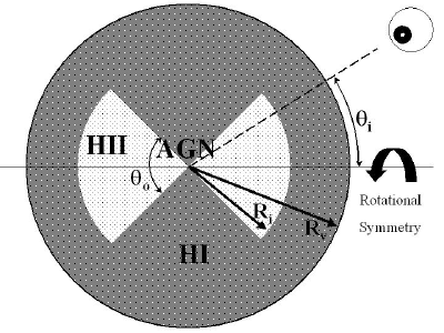
Figure 2: The geometry of our simulation. $\theta_{i}$ is the inclination as constrained by Carilli (1995). $R_{v}$ is the system’s virial radius. $R_{i}$ is the ionization radius of the cones. $\theta_{o}$ is the opening angle of the ionization cones assumed here to be $90\arcdeg$. $R_{i}$, $R_{v}$, $\theta_{o}$, and two variables controlling the velocity field are the model’s five tunable parameters.

The basic geometry we investigate is shown in Figure 2. This scenario is based on a proposal in van Ojik et al. (1997), although that work does not investigate the key effects of resonant scattering. The Lyman-$\alpha$ emission in HzRGs is often strongest along the radio axis in a biconal geometry. This geometry has been advocated on AGN ionizing photon counting grounds (McCarthy & van Breugel, 1989) and for AGN unification models (Barthel, 1989; Antonucci, 1993). Surrounding the cones is a large halo of neutral hydrogen gas. Our model postulates an opening angle of 90$\arcdeg$ for each cone. Matching the spatial location of the bimodal emission in our data and that of Reuland et al. (2007), we model the projection of the emission cones axis on the sky at 60$\arcdeg$ east of north. It is not clear from the radio data exactly where the radio axis projects, but given the large deprojection uncertainty in such a low inclination system and the complex bending of the radio image, this geometry is reasonable. The ionization cone radius could be constrained by the Lyman-$\alpha$ luminosity, but since the filling factor is highly uncertain we keep this radius as an open parameter. We model the density profile as baryons at 17$\%$ of the total mass following Navarro-Frenk-White (NFW) profiles (Navarro et al., 1997) with a thermal core and concentration parameters of c = 5 following Dijkstra et al. (2006a), hereafter DHS. The input velocity field is parameterized as a simple power law with $v_{bulk}=v_{amp}\times v_{vir}\times(r/r_{vir})^{\alpha}$ where $\alpha$ is the index, $r$ is radius, $r_{vir}$ is the virial radius, $v_{vir}$ is the virial velocity, and $v_{amp}$ is a scaling factor of order one. The input parameters and acceptable ranges we explore in common to DHS are total halo mass, $v_{amp}$, and $\alpha$. The halo is isothermal at $10^{4}$K, and the neutral fraction in the ionization cones is $10^{-4}$, both appropriate to the common ranges of density in photoionized regions. We model a completely smooth distribution of gas as a simplifying assumption. In a very similar type of problem, low redshift cooling flows, Fabian et al. (1984) have shown how smooth flow assumptions adequately model infalling gas. The linear relation between the average number of photon scatterings before escape and the line center optical depth as shown in Appendix A ensures that gas clumping is irrelevant to our results.

3.2 Resonant Scattering Model

Given our new data of spatially resolved two dimensional Lyman-$\alpha$ emission, we have sufficient information to create a simple model for this system based on propagation of Lyman-$\alpha$ photons through an optically thick halo of HI with geometry as in Figure 2. Lyman-$\alpha$ radiative transfer is a mature field (Harrington, 1973; Urbaniak & Wolfe, 1981; Neufeld, 1991; Loeb & Rybicki, 1999; Ahn et al., 2000, 2001, 2002; Zheng & Miralda-Escudé, 2002; Richling, 2003; Hansen & Oh, 2006; Dijkstra et al., 2006a, b; Verhamme et al., 2006; Tasitsiomi, 2006; Laursen et al., 2008) with both analytic and computational results for simple geometries. Broadly, the model will work by emitting Lyman-$\alpha$ photons in two photoionized cones roughly aligned with the radio axes. A red and blue emission line relative to systemic will emerge for each cone absent a velocity field in the scattering gas giving four peaks in the line profile. The far cone’s emission will be weaker and further from the HzRGs systemic redshift. Global dynamics of infall will enhance the two blue emission peaks and suppress the two red emission peaks. Outflow will produce a mirror image spectrum about the systemic redshift and suppress the two blue emission peaks and enhance the two red emission peaks. The relative wavelengths between the stronger, narrower emission from the near cone and the weaker, broader emission from the rear cone can then discriminate between infall and outflow even if the systemic redshift is unknown. This method provides constraints on the HI mass and velocity field by measuring the bimodal line properties and the systemic redshift if available.

The study of Lyman-$\alpha$ resonant scattering can be profitably attacked through Monte Carlo methods. We base our computations primarily on DHS, where DHS used Monte Carlo methods to attempt discrimination between energy sources and conditions in the data on LABs. Our version of the Monte Carlo resonant scattering code differs in three ways from their description. First, we do not include deuterium in our simulations. Although they show convincingly that deuterium is important for certain wavelengths and conditions, our very high optical depth and temperature environments make its contribution negligible and a needless drain on computing performance. Second, all of DHS’s geometries are restricted to spherical symmetry. As we will invoke the two cones of the AGN as coaxial with the cones of Lyman-$\alpha$ emission, our models are without spherical symmetry. Our simulations therefore are a function of inclination angle and require the same number of simulation photons in each inclination angle bin as in an entire DHS simulation to reach an equal S/N. Third, DHS have a geometry that yields an analytic expression between optical depth and traversed physical distance for thin shells of constant density and velocity gas. The general density and velocity field conditions in our model mean that we must integrate this distance numerically. We use a root finding algorithm with a relative accuracy of $10^{-8}$ on a fifth order Runge-Kutta code to calculate optical depths and sites of scatter. It is this generalization that enables us to pursue arbitrary density, temperature, and velocity fields. It will be possible to leverage this generalization by coupling our code to the more realistic conditions output by hydrodynamic codes in future work, but for now we use relatively ad hoc parameterizations. We used, in common with DHS, an acceleration scheme with x${}_{crit}=3$ as described in their §3.1.1. Our simulation work is an extension and application of the powerful method of DHS to a different class of object, HzRGs. We have run our code for the four test cases shown in DHS’s Figure 1 and found agreement as demonstrated in Appendix A.

Our main differences in operation from the DHS models are the changes in HI density in the presence of ionization cones and AGN photoionization as the dominant Lyman-$\alpha$ energy source determining the emissivity profile. Lyman-$\alpha$ emission powered by a cooling flow and its associated uncertainties are unnecessary in B2 0902+34 with the strong evidence for AGN photoionization. Within the ionization cones, Lyman-$\alpha$ is generated randomly in position following the recombination rate.

Our simulation ends when a photon leaves the virial radius. Further radiative transfer effects in the IGM are beyond this work’s scope, although they can be important (Dijkstra et al., 2006b; Barkana, 2004). We briefly discuss the qualitative impact that IGM processing by infalling neutral hydrogen outside the virial radius could have to our model. Figure 2 of Dijkstra et al. (2006b) gives transmission curves at $z=3$ for a variety of impact parameters and for cases with and without a nearby bright, ionizing quasar. Multiplying this transmission into a single peaked emission profile can produce a bimodal line profile, but this is not a likely explanation by itself for B2 0902+34. Only emission lines that are well centered around the systemic redshift can be modified by the IGM into a bimodal profile as the transmission minimum occurs slightly redward of systemic. All our models produce Lyman-$\alpha$ emission that is blueshifted enough that the IGM processing could not create a bimodal spectrum. The higher 21 cm redshifts also imply that the Lyman-$\alpha$ emission is not near the systemic redshift. We also do not observe the spatial dependence with impact parameter that IGM processing would create. For these reasons and scope, we neglect IGM processing.

We must review a few of the broad findings in DHS to understand our models. Radiative escape from a static gas cloud will produce a bimodal spectrum. A photon has a much longer mean free path when it is at an off-resonance wavelength, which the thermal kicks in a scatter can cause. This situation will produce peaks redward and blueward of systemic with higher optical depths pushing the peaks out to more separated wavelengths. If the same situation has global infall (outflow) in the scattering gas, the photon moving outward and being scattered will have on average a blue-(red-)shift in the frame of the atom. A photon formerly in the red (blue) wing will move into resonance and have its travelling distance supressed, while a photon formerly in the blue (red) wing will be pushed further into the scattering wing and travel further before its next scatter. In practice, the suppressed emission peak is likely to be far below detection limits for the range of optical depths we investigate. Therefore we return to a solitary emission line with no information remaining on the system’s systemic redshift for cases of spherical symmetry. As DHS acknowledge, there is a degeneracy in observation between systems in infall and outflow. We turn to a stark physical difference between the DHS modeled LABs and our HzRGs to solve this problem. HzRGs frequently have two discrete regions of emission as ionization cones powered by the AGN. In a low inclination angle system such as B2 0902+34, the optical depth difference between these two regions to an observer can be substantial. Such a system should exhibit a weaker, spatially restricted emission profile caused by the rear ionization cone superimposed on a stronger, nearly circularly distributed emission profile caused by the near ionization cone. The relative order in wavelength between the weak and strong emission peaks will point in the direction of the unobserved, systemic redshift. So, HzRGs may be unique as high redshift halos where observation can distinguish without ambiguity between infall and outflow, solely from Lyman-$\alpha$ emission profiles. B2 0902+34 provides a further test of this idea since it is the only HzRG with a detection of 21 cm HI absorption.

3.3 Evaluation of Model

In Figure 3 we give the observed and simulated spectra in identical apertures for a particular model. There are five tunable parameters to our model: the virial radius, the ionization radius, the velocity strength, the power law index to the velocity field, and the photoionized cones’ opening angle. We have coarsely run models over the likely halo parameter space, but we only present one model which captures many of the necessary observed traits. This model realization uses 700,000 photons generated in a $6\times 10^{12}$M_☉ halo which corresponds to a virial radius of 134 kpc and a virial velocity of 437 km s^-1. The ionization radius extends to 101 kpc for this realization. We use an infall model where the velocity varies as the radius to the power $\alpha$ where here $\alpha=0.5$ and with a maximum radially inward velocity at the virial radius of 656 km s^-1. The cone opening angle is 90$\arcdeg$. We have one further parameter which we hold constant as it is well constrained by a previously discussed observation: the system’s inclination angle. We believe $\theta_{i}=45\arcdeg$ as most likely given the absence of an observed broad line region, so in practice we bin the spatial projections and wavelengths for all photons that exit within 35$\arcdeg$ to 55$\arcdeg$ of an ionization cone axis. For our model, we have assumed a systemic redshift of $z_{systemic}=3.3990$. We have done this after judging the velocity offset that the 21 cm absorption measurement should have in §3.4. The various redshifts are reviewed in Table 4.

This model reproduces many features of the observation. Most importantly, the size of the split in wavelength between the primary and secondary peak is recovered in the bottom panel of Figure 3. The relative intensities between the primary (near cone) and secondary (rear cone) emission are also fairly well matched. The regions of the halo not in projection of the receding radio cone also show the proper behavior as demonstrated in the top plot of Figure 3. The emission there is not bimodal, and the peak is nearly constant at the same wavelength as the redder peak in the bimodal region. Several features in the model clearly do not meet the data, and our model is not to be considered the optimum match in parameter space but instead an early attempt. The model data all display a blueward skew, especially in Fiber 4 (top panel, Figure 3) and regions away from either photoionized cone. Our data’s S/N does not allow a useful measure of skew, but we predict that a much deeper and perhaps higher spectral resolution observation would show skew. This lack of skew is currently the most outstanding mismatch between our model and data.

We consider our results as surface brightness distributions in Figure 4. The left panel shows the observed decomposition between the primary and secondary peaks. The middle panel shows a similar decomposition for our model, where emission is decomposed spectrally. The right panel shows the model with the emission decomposed by the photoionized cone of origin. When we fairly decompose the model as in the middle panel, the region of secondary emission is pushed out slightly from the HzRG center and the relative intensity from secondary emission is underpredicted. Other models we have run have matched the spatial contours more closely, but have other failings such as underpredicting the bimodal wavelength separation, giving much broader lines, or showing even more skew. The modest S/N’s so far observed for this dim object will inevitably cause confusion between skew, line width, and a bimodal line profile, so our unoptimized model parameter choices are appropriate to the state of certainty in the current data. The spatial distributions and relative intensities are fairly well matched at the level of the coarse spatial sampling allowed by our observation’s fiber size. The offset spatial peak from the near ionized cone is also a robust match and explains why the Lyman-$\alpha$ peak and the radio core do not coincide.

Other parameter choices have some important trends. We cannot use a much smaller total halo mass, because the rest frame wavelength separation in the bimodal regions drops from 4Å to 1Å for a total halo mass of $3\times 10^{12}$M_⊙. Larger halo masses are allowed and give more freedom in the other model parameters to reach the crucial rest frame wavelength separation of 4Å, so we consider our gas mass to be a lower limit. Larger $\alpha$ values produce narrower emission lines with more skew, while a value of -0.5 creates lines of huge (40Å) dispersion and spectral shifts (thousands of km s^-1 from systemic) that are incompatible with the data. Smaller $R_{i}$ to $R_{v}$ ratios seem to also lower the rest frame 4Å line profile separation unacceptably. A smaller value of $\theta_{o}=60\arcdeg$ gives the appealing feature of more cleanly separating the near and rear photoionized cones spectrally much as the right panel of Figure 4 shows, but the emission not in projection of the near cone begins to show line centers improperly centered around the wavelength of secondary emission contrary to observation. The most robust result of these models is that a rest frame line separation of 4Å can be accomplished with resonant scattering from HzRG cones with a very large HI mass ($10^{12}$M_⊙), but a separation of much more (say, 8Å) can not without masses an order of magnitude larger.

Table 4: Redshift estimates in B2 0902+34

Primary Lyman-$\alpha$	Secondary Lyman-$\alpha$	21 cm absorption	Systemic from model
3.3918	3.3795	3.3962	3.3990

3.4 21 cm Predictions

Any correct physical model of B2 0902+34 must take account of the 21 cm absorption data. Table 3 shows that fits of absorption to the Lyman-$\alpha$ line profile do not match the absorbing population of HI evident in the 21 cm data. Cody & Braun (2003) detect an absorption feature of FWHM 120 km s^-1 at z = 3.3962 with a column density of $3\times 10^{21}$ cm^-2 under an assumed spin temperature of T_s=10³K. The relative velocities between the Lyman-$\alpha$ emission and the 21 cm absorbing HI and the absence of a signature from the 21 cm absorping gas in the Lyman-$\alpha$ profile both give strong constrains on possible geometries and conditions.

Our model naturally reproduces the 21 cm absorption measurements without the need for a counterpart dip in the Lyman-$\alpha$ profile. By embedding the emission sites of Lyman-$\alpha$ in a larger neutral halo, the effects of scattering will not leave an absorption-like imprint on the Lyman-$\alpha$ profile, but they will do so on the 21 cm profile against the radio continuum emission. All existing 21 cm data on B2 0902+34 are spatially unresolved. Figure 6 predicts the 21 cm maps that could be made using radio interferometry. The exact source distribution at 21 cm (323 MHz observed frame) is unknown, but we estimate it to be the same as the 1.65 GHz distribution of Carilli (1995). We assume the radio source plane to be the sky plane rotated onto the radio axis at an inclination of 45$\arcdeg$. We use the same model parameters as introduced in §3.3. We find a column density of 1.0$\times 10^{21}$ to 1.0$\times 10^{22}$cm^-2, a dispersion of 135 to 210 km s^-1, and a velocity shift from systemic of -190 to -275 km s^-1. These column densities would make this object a Damped Lyman-$\alpha$ system with a radius $>50$ kpc. The highest intensity radio emission resides is in a region of large gradients for the absorption properties, so slight changes in source distribution or rotation in the plane of the sky cause large changes in the integrated values. We give the ranges that misalignments of $\pm$1$\arcsec$ can create. The predicted line width is a factor of 2 above the measurement, but the rather unconstrained $\alpha$ parameter in the velocity field could likely remedy the mismatch as it takes a value closer to zero. Otherwise, the observations are bounded by these ranges, and the velocity shift tells us that our model self-consistently has both Lyman-$\alpha$ emission peaks blueward of both the 21 cm redshift and the systemic redshift. It is the velocity shift of 190 km s^-1 for our fiducial astrometry that led us to the earlier assertion of $z_{systemic}=3.3990$. When building our resonant scattering model, we only let the 21 cm measurements guide our choice of systemic redshift. It is encouraging that our model designed to match the bimodal Lyman-$\alpha$ line profiles recovers so well the spatially unresolved 21 cm absorption signatures.

Our most robust prediction comes from the southern radio lobe. Approximately 10% of the radio signal originates from this region in a $\sim$1$\arcsec$ diameter aperture judging from the 1.65GHz data. Assuming the absorption strength is uniform over the halo, this aperture should have an absorption strength of 1.6mJy. Spatially resolved observations would need an unattainably long 1100 hours of exposure with 4 dishes from the Very Long Baseline Array (VLBA) and the phased Very Large Array (VLA) to reach the same S/N of 6 as in the spatially unresolved absorption measurement (Cody & Braun, 2003) at a spectral resolution of 62.5kHz (restframe 58km s^-1) around the 323.053MHz observed frequency according to the European VLBI Network calculator. Adding more VLBA dishes or other facilities, such as Greenbank or Arecibo, does not lower the exposure time as the increased baselines overresolve the southern lobe. However, the brighter northern jet could be measured at a S/N of 5 in 40 hours under the same configuration, and we are pursuing that observation. A spatially resolved 21cm measurement will give important confirming or falsifying evidence for a vast and massive infalling gas halo.

4 Implications: Infall Versus Outflow

We are left with two serious, competing pictures: outflow from a 100 kpc HII region or infall of a 100 kpc HI region with embedded cones of HII. Deciding between these mechanisms has impact beyond B2 0902+34. The bimodal line profile we see in B2 0902+34 is fairly common in HzRG halos. van Ojik et al. (1997) found 11 of 18 such systems to carry the feature in longslit spectroscopy, although they all have not been studied for the confirming 2D spatial profiles as can be done with IFS.

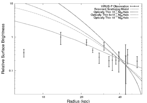
Figure 7: Observed and simulated surface brightness profiles. All models have been scaled in intensity by least squares to the data. The optically thin integrals through NFW halos fail, though the resonant scattering model reproduces the observed, shallower profile.

The outflow picture requires shells or clumps of HI at a large radius from the emission halo. This gas scatters a fraction of the line emission, and the blueshift in the absorption trough argues for outflow. The energy mechanism might be a starburst-driven superwind as discussed above. Wilman et al. (2005) has applied such an explanation to LAB2 as has Reuland et al. (2007) for several HzRGs including B2 0902+34. If correct, these systems may be showing feedback in action with gas being heated and driven out. We see three reasons that this model is likely inappropriate to B2 0902+34. First, the 21 cm absorbing HI has no natural home in this picture. The radio emission, which extends to $\approx$40 kpc must lie behind this bit of HI, but the Lyman-$\alpha$ photons must be generated in front or must at least have many scatterings after the absorption as no spectra shows Lyman-$\alpha$ absorption at the 21 cm redshift and column density. Reuland et al. (2007) recognize this and predict a small, dense cloud of HI around the AGN. This too is unlikely, as the amount of spectrally flat radio core emission available for absorption in the data of Carilli (1995) and the amount required by the 21cm measurement of Cody & Braun (2003) are modestly incompatible. Second, the surface brightness profile has the wrong slope for unscattered, extended emission. As shown in Figure 7, the observed surface brightness profile follows a power law. Taking an NFW profile for density and integrating the square of the density through the halo, assuming an optically thin case and highly extended photoionization, we find surface brightness profiles that are too steep for all reasonable halo masses. Our simulation of resonant scattering gives a nearly power law profile with an appropriate slope. Third, the geometry of an absorbing cloud would have to be finely tuned to produce the observation. Based on our spectroscopy and that of Reuland et al. (2007), the primary peak’s center stays very constant at 5339.0 $\pm$ 2.0Å in all positions. In the NE, there is no secondary emission peak so the absorption must be total and go quite blue. In the SW, the absorption would have to be weaker, narrower, and redder than in the NE to produce Figure 4 of Reuland et al. (2007). The outflow picture does not produce a natural explanation for the spatial variation in the line profile.

Our result is surprising compared to the study of Nesvadba et al. (2008) with data from three other HzRGs. The authors find extended emission in rest-frame optical lines and kinematics indicative of outflow. A possibly crucial difference between the datasets is that for B2 0902+34 the emission line regions extend far beyond the radio lobes, while the other three HzRGs are bounded by radio emission and significantly elongated along the radio axis. If we speculate that both our and their conclusions are true, the next questions becomes whether the same HzRGs show different dynamical signatures through different lines or whether different HzRGs show different dynamical signatures across all their lines.

The infall picture has been suggested before for HzRGs (e.g. Humphrey et al., 2007). Villar-Martín et al. (2007b) produced a model of optically thin biconal emission in Lyman-$\alpha$ to recover their observations of a peak emission position and peak velocity offset position. Their models, however, required postulation of a dense core that blocks emission from a rear cone that would have upset their trends, so their model is inappropriate to a bimodal line profile. They also could not produce lines at the width of their observations. We agree with the infall picture but use an optically thick regime of ionization cones embedded in one large, continuous neutral halo to explain all the available data on B2 0902+34 as we discussed above. If correct, this method has the capability to measure distributed hydrogen mass which we predict to be of the order $10^{12}M_{\odot}$. This is 5 orders of magnitude higher than the warm and cool hydrogen populations estimates by De Breuck et al. (2003) for the HzRG J2330+3927 from optically thin assumptions and Lyman-$\alpha$ line profile absorption specifically, and similarly high for the typical mass budget of HzRGs (Miley & De Breuck, 2008). The neutral gas mass is dominant by a factor of $\geq$17 compared to the estimate of stellar mass in B2 0902+34 of $6\times 10^{10}M_{\odot}$ (Seymour et al., 2007). We note that in the work of Seymour et al. (2007), B2 0902+34 has an usually low stellar mass compared to other radio galaxies at a similar epoch. Combined with our work here, this low stellar mass may indicate HzRGs exist in a fairly heterogeneous range of galaxy evolution, with B2 0902+34 at an earlier stage of evolution than the average HzRG. The unusually early evolutionary state and large HI halo for B2 0902+34 may also be why only B2 0902+34 so far has shown 21 cm absorption. Our model also puts the system in a radically different evolutionary state from that predicted by outflow. Instead, we have infalling gas that is still building up what will become the galaxy’s luminous mass. Star and dust formation have not yet built up to a dominant level to affect the Lyman-$\alpha$ line. The central AGN has not yet blown out or heated a significant fraction of its environment in an act of feedback. The model mass would place B2 0902+34 as one of the larger halos that should collapse at the observed redshift. This picture does not deny HzRGs the role of feedback agents, but does show that radio emission can be output in a protogalactic phase as well and that AGN buildup may predate significant star formation. Further study on B2 0902+34 may be important in deciding the origin of supermassive black holes (Djorgovski et al., 2008), and their coevolution with stellar bulges. Two likely paths of early black hole formation are as end biproducts of the earliest stars (Madau & Rees, 2001; Ricotti & Ostriker, 2004) or as gas that avoided molecular cooling and fragmentation and collapsed into a black hole without associated star formation (Silk & Rees, 1998; Loeb & Rasio, 1994; Eisenstein & Loeb, 1995; Bromm & Loeb, 2003; Koushiappas et al., 2004). In the latter case, a phase of galaxy evolution may exist where the stellar bulge and black hole masses are not tightly related. Although we do not have an estimate of B2 0902+34’s black hole mass, the large radio continuum luminosity suggests an already large black hole. B2 0902+34, although we do not observe any associated cluster LAEs, may yet grow into a rich cluster as the normal cluster members begin their own star formation, possibly triggered by B2 0902+34 itself as described in Rawlings & Jarvis (2004).

While we advocate a resonantly scattering, infalling model to explain the extent of emission and the otherwise conflicting Lyman-$\alpha$ and 21cm absorption data, our model does require a minimum of $10^{12}M_{\odot}$ in HI subject to the modeled constraint of a maximum infall velocity of $v_{bulk}=v_{amp}\times v_{vir}\times(r/r_{vir})^{\alpha}$ with here $v_{amp}\leq 1.5$. Having this much HI inside a galaxy’s virial radius conflicts with the classic galaxy formation scenario (Binney, 1977; Rees & Ostriker, 1977; Silk, 1977). In that picture, a shock near the virial radius should ionize incoming gas and heat it to $\approx 10^{6}K$ where it stays in quasi-hydrostatic equilibrium. Especially in the most massive halos, the low density gas is expected to have a cooling time longer than the galaxy age. This scenario has been adjusted in recent years with rapidly cooling accretion flows showing up in semi-analytic simulations (Croton et al., 2006) and cold accretion in smoothed particle hydrodynamics (SPH) simulations where a virial shock is mass conditionally unstable (Birnboim & Dekel, 2003) and filaments provide many paths where cold gas ($<10^{5}K$) can flow to the forming galaxy’s center (Fardal et al., 2001; Kereš et al., 2005; Dekel & Birnboim, 2006; Dekel et al., 2008; Kereš et al., 2008; Ocvirk et al., 2008). The ability of cooling and cold flows to exist have a redshift and halo mass dependence. Croton et al. (2006) give $M_{halo}<2-3\times 10^{11}M_{\odot}$ for z=0-6 and Kereš et al. (2005) give $M_{halo}<10^{11.4}M_{\odot}$ at z=0 with some redshift evolution. In either case, our advocacy for a $M_{halo}>5\times 10^{12}M_{\odot}$ at z=3.4 appears to be in conflict with theory. Instead, the growth mechanism of such a massive halo is expected to be mergers. Future radiative transfer simulations of Lyman-$\alpha$ in more realistic, filament conditions may alleviate this mismatch in mass scale, although since the velocity fields in Kereš et al. (2005) are of the same order as those we modeled, an easy solution is not obvious. The potential conflict with theory at such a large mass makes B2 0902+34 a compelling target for further observations and simulations.

5 Conclusions

We have made new spatially resolved IFS observations of Lyman-$\alpha$ in B2 0902+34. We find a spatially resolved region of weaker and bluer emission superimposed on a symmetric halo of primary emission. We have shown that all properties of B2 0902+34 can best be fit with a resonant scattering infall model with a large, mostly neutral, hydrogen mass. The sign of the velocity field is relatively robust and model independent. Signal seen through higher optical depths becomes increasingly bluer indicative of infall and resonant scattering. We match our data with a model dependent HI mass of $\geq 10^{12}M_{\odot}$ which is $\geq$17$\times$ larger than the stellar mass. For three reasons an outflowing HI scenario cannot fit our observations: 1) the strength of the observed 21cm absorption and the Lyman-$\alpha$ profile are incompatible with a single HI population if optically thin and the velocity offsets between the 21cm signal and the higher optical depth Lyman-$\alpha$ signal carry the wrong sign for outflow if optically thick, 2) the surface brightness profile, with the assumption that the gas follows the dark matter, would be steeper than observed if optically thin, and 3) the bimodal Lyman-$\alpha$ line profile exists only in a small, non-central region of the galaxy which is incompatible with an outflowing shell geometry. The 21 cm HI absorption has been a powerful confirmation of the kinematics through its redshift offset from the Lyman-$\alpha$ halo emission, and we believe observational progress in understanding this class of object will benefit from further deep 21 cm measurements on other HzRGs. This new scenario of a massive, infalling HI halo with resonant scattering places B2 0902+34 in a much earlier evolutionary state than the previously formulated starburst superwind picture, and we classify B2 0902+34 as a protogiant elliptical galaxy in an early collapse phase before significant feedback has disrupted star formation and AGN fueling. Observations of other HzRGs with IFS will be important in correctly classifying systems between formation and feedback modes and allow detailed observational tests of these two processes. We are observing a large sample of HzRGs with VIRUS-P in order to undertake a similar analysis on other systems.

Further types of data on this system will allow confirmation of our infalling, resonant scattering model. Polarization measurements of Lyman-$\alpha$ could confirm the scattering process (Lee & Ahn, 1998). The bright regions of HzRGs have been found to have modest levels of polarization ($\approx$10%, Vernet et al. (2001)) while scattering simulations in similar situations to our model (Dijkstra & Loeb, 2008) predict higher ($\approx$40%) values. A measurement between HzRGs with and without emission line halos may demonstrate this split. The key, potentially falsifying observation for this resonant scattering, infalling model of B2 0902+34 will be radio interferometry spectral imaging to spatially resolve the distribution of HI gas through its 21 cm absorption. Carilli (1995) discussed the utility of such a measurement, and we have now given an observationally motivated model that predicts spatially extended HI.

Appendix A Tests of the resonant scattering code

To provide compatibility between our work and previous authors’, we run the same set of four tests on our 3D Monte Carlo resonant scattering code as Dijkstra et al. (2006a). The first test simulates the emergent spectra for centrally created Lyman-$\alpha$ photons in a uniform density spherically symmetric static halo of HI with various line center edge-to-center optical depths at T=10K. We disabled the acceleration scheme for tests 1-3. The second test calculates the redistribution function for single scattering events, which is the probability distribution function for an output frequency given an input frequency and gas temperature. The third test finds the mean number of scatterings prior to escape for a slab of gas of various line center optical depths. The weighting scheme of Avery & House (1968) was used for test 3 where the number of accumulated scatterings and the probability of escape from each scattering site is retained as opposed to solely keeping the properties of each Monte Carlo run’s escaping photon. The fourth test gives the emergent spectrum from an infinitely large object under Hubble expansion as originally simulated in Loeb & Rybicki (1999). More details and references are given in Dijkstra et al. (2006a) Appendix B. We give the four tests in Figure 8.

Figure 3: The spectra of both our IFS data and resonant scattering simulation from select fibers. The thin dotted line indicates the redshift measured for 21 cm absorption. Solid Observed. Thick dotted Simulated. Top Fiber 4, representative of most of the halo area where neither cone directly projects. Middle Fiber 7, representative of regions spanned by the near photoionized cone. Bottom left Fiber 14, representative of regions spanned by the rear photoionized cone. Only these regions show a bimodal line profile. Bottom right A region in the simulation near fiber 14. While we did not have a fiber on this exact position, the bimodal spectrum here is a good match to its neighbor in fiber 14.

Figure 6: The predicted 21 cm maps for B2 0902+34. The 1.65 GHz data of Carilli (1995) is plotted as the dashed contour as a likely source distribution. Top Left Column density where the log of N(HI) in cm^-2 is given. Top Right Velocity dispersion in km s^-1. Bottom Velocity shift in km s^-1.

Figure 8: The four tests of our 3D Monte Carlo resonant scatter code. Top left The emergent Lyman-$\alpha$ spectra from uniform density, static halos at T=10K with various line center edge-to-center optical depths. The histograms are from our simulations. The lines are from function 9 in Dijkstra et al. (2006a). Top right The redistribution function for Lyman-$\alpha$ scattering with a gas temperature of T=10⁴K. The histogram is our code output while the curves are from theory in Hummer (1962); Lee (1974). Bottom left The number of scatterings necessary for a Lyman-$\alpha$ photon to escape a neutral, static slab of HI. The points are from our simulations. The line is from theory (Harrington, 1973). Bottom right The emergent Lyman-$\alpha$ spectrum from an infinite, uniform density HI halo under Hubble expansion at z=10 with T=10K.

References

- Adam et al. (1997) Adam, G., Rocca-Volmerange, B., Gerard, S., Ferruit, P., & Bacon, R. 1997, A&A, 326, 501
- Ahn et al. (2000) Ahn, S.-H., Lee, H.-W., & Lee, H. M. 2000, Journal of Korean Astronomical Society, 33, 29
- Ahn et al. (2001) Ahn, S.-H., Lee, H.-W., & Lee, H. M. 2001, ApJ, 554, 604
- Ahn et al. (2002) Ahn, S.-H., Lee, H.-W., & Lee, H. M. 2002, ApJ, 567, 922
- Ahn & Lee (2002) Ahn, S.-H., & Lee, H.-W. 2002, Journal of Korean Astronomical Society, 35, 175
- Antonucci (1993) Antonucci, R. 1993, ARA&A, 31, 473
- Arnaud & Evrard (1999) Arnaud, M., & Evrard, A. E. 1999, MNRAS, 305, 631
- Avery & House (1968) Avery, L. W., & House, L. L. 1968, ApJ, 152, 493
- Barkana & Loeb (2003) Barkana, R., & Loeb, A. 2003, Nature, 421, 341
- Barkana (2004) Barkana, R. 2004, MNRAS, 347, 59
- Barthel (1989) Barthel, P. D. 1989, ApJ, 336, 606
- Begelman & Cioffi (1989) Begelman, M. C., & Cioffi, D. F. 1989, ApJ, 345, L21
- Best (2000) Best, P. N. 2000, MNRAS, 317, 720
- Binney (1977) Binney, J. 1977, ApJ, 215, 483
- Birnboim & Dekel (2003) Birnboim, Y., & Dekel, A. 2003, MNRAS, 345, 349
- Briggs et al. (1993) Briggs, F. H., Sorar, E., & Taramopoulos, A. 1993, ApJ, 415, L99
- Bromm & Loeb (2003) Bromm, V., & Loeb, A. 2003, ApJ, 596, 34
- Carilli (1995) Carilli, C. L. 1995, A&A, 298, 77
- Carilli et al. (1997) Carilli, C. L., Roettgering, H. J. A., van Ojik, R., Miley, G. K., & van Breugel, W. J. M. 1997, ApJS, 109, 1
- Chambers & Miley (1990) Chambers, K. C., & Miley, G. K. 1990, Evolution of the Universe of Galaxies, 10, 373
- Chandra et al. (2004) Chandra, P., Swarup, G., Kulkarni, V. K., & Kantharia, N. G. 2004, Journal of Astrophysics and Astronomy, 25, 57
- Cody & Braun (2003) Cody, A. M., & Braun, R. 2003, A&A, 400, 871
- Cooke et al. (2008) Cooke, J., Barton, E. J., Bullock, J. S., Stewart, K. R., & Wolfe, A. M. 2008, ApJ, 681, L57
- Croton et al. (2006) Croton, D. J., et al. 2006, MNRAS, 365, 11
- De Breuck et al. (2003) De Breuck, C., et al. 2003, A&A, 401, 911
- De Breuck et al. (2005) De Breuck, C., Downes, D., Neri, R., van Breugel, W., Reuland, M., Omont, A., & Ivison, R. 2005, A&A, 430, L1
- Dekel & Birnboim (2006) Dekel, A., & Birnboim, Y. 2006, MNRAS, 368, 2
- Dekel et al. (2008) Dekel, A., et al. 2008, arXiv:0808.0553
- Dierckx (1993) Dierckx, P. 1993, Curve and Surface Fitting with Splines, Clarendon Press, New York, 1993
- Dijkstra et al. (2006a) Dijkstra, M., Haiman, Z., & Spaans, M. 2006, ApJ, 649, 14
- Dijkstra et al. (2006b) Dijkstra, M., Haiman, Z., & Spaans, M. 2006, ApJ, 649, 37
- Dijkstra & Loeb (2008) Dijkstra, M., & Loeb, A. 2008, MNRAS, 386, 492
- Djorgovski et al. (2008) Djorgovski, S. G., Volonteri, M., Springel, V., Bromm, V., & Meylan, G. 2008, ArXiv e-prints, 803, arXiv:0803.2862
- Eales et al. (1993) Eales, S., Rawlings, S., Puxley, P., Rocca-Volmerange, B., & Kuntz, K. 1993, Nature, 363, 140
- Eisenhardt & Dickinson (1992) Eisenhardt, P., & Dickinson, M. 1992, ApJ, 399, L47
- Eisenstein & Loeb (1995) Eisenstein, D. J., & Loeb, A. 1995, ApJ, 443, 11
- Fabian et al. (1984) Fabian, A. C., Nulsen, P. E. J., & Canizares, C. R. 1984, Nature, 310, 733
- Fabian (1994) Fabian, A. C. 1994, ARA&A, 32, 277
- Fan et al. (2003) Fan, X., et al. 2003, AJ, 125, 1649
- Fardal et al. (2001) Fardal, M. A., Katz, N., Gardner, J. P., Hernquist, L., Weinberg, D. H., & Davé, R. 2001, ApJ, 562, 605
- Ferrarese & Merritt (2000) Ferrarese, L., & Merritt, D. 2000, ApJ, 539, L9
- Gebhardt et al. (2000) Gebhardt, K., et al. 2000, ApJ, 539, L13
- Haiman et al. (2000) Haiman, Z., Spaans, M., & Quataert, E. 2000, ApJ, 537, L5
- Hansen & Oh (2006) Hansen, M., & Oh, S. P. 2006, MNRAS, 367, 979
- Harrington (1973) Harrington, J. P. 1973, MNRAS, 162, 43
- Hayes et al. (2007) Hayes, M., Östlin, G., Atek, H., Kunth, D., Mas-Hesse, J. M., Leitherer, C., Jiménez-Bailón, E., & Adamo, A. 2007, MNRAS, 382, 1465
- Heckman et al. (1991) Heckman, T. M., Lehnert, M. D., Miley, G. K., & van Breugel, W. 1991, ApJ, 381, 373
- Heckman (2002) Heckman, T. M. 2002, Extragalactic Gas at Low Redshift, 254, 292
- Hill & Lilly (1991) Hill, G. J., & Lilly, S. J. 1991, ApJ, 367, 1
- Hill et al. (2008) Hill, G. J., et al. 2008, Proc. SPIE, 7014, 257
- Hummer (1962) Hummer, D. G. 1962, MNRAS, 125, 21
- Humphrey et al. (2007) Humphrey, A., Villar-Martín, M., Fosbury, R., Binette, L., Vernet, J., De Breuck, C., & di Serego Alighieri, S. 2007, MNRAS, 375, 705
- Inoue & Sasaki (2001) Inoue, S., & Sasaki, S. 2001, ApJ, 562, 618
- Kaastra et al. (2001) Kaastra, J. S., Ferrigno, C., Tamura, T., Paerels, F. B. S., Peterson, J. R., & Mittaz, J. P. D. 2001, A&A, 365, L99
- Kaiser (1986) Kaiser, N. 1986, MNRAS, 222, 323
- Keel et al. (1999) Keel, W. C., Cohen, S. H., Windhorst, R. A., & Waddington, I. 1999, AJ, 118, 2547
- Kelson (2003) Kelson, D. D. 2003, PASP, 115, 688
- Kennicutt (1998) Kennicutt, R. C., Jr. 1998, ARA&A, 36, 189
- Kereš et al. (2005) Kereš, D., Katz, N., Weinberg, D. H., & Davé, R. 2005, MNRAS, 363, 2
- Kereš et al. (2008) Keres, D., Katz, N., Fardal, M., Dave, R., & Weinberg, D. H. 2008, arXiv:0809.1430
- Koushiappas et al. (2004) Koushiappas, S. M., Bullock, J. S., & Dekel, A. 2004, MNRAS, 354, 292
- Kunth et al. (1998) Kunth, D., Mas-Hesse, J. M., Terlevich, E., Terlevich, R., Lequeux, J., & Fall, S. M. 1998, A&A, 334, 11
- Laursen et al. (2008) Laursen, P., Razoumov, A. O., & Sommer-Larsen, J. 2008, arXiv:0805.3153
- Le Fevre et al. (1996) Le Fevre, O., Deltorn, J. M., Crampton, D., & Dickinson, M. 1996, ApJ, 471, L11
- Lee (1974) Lee, J.-S. 1974, ApJ, 192, 465
- Lee & Ahn (1998) Lee, H.-W., & Ahn, S.-H. 1998, ApJ, 504, L61
- Li et al. (2007) Li, Y., et al. 2007, ApJ, 665, 187
- Lilly & Longair (1984) Lilly, S. J., & Longair, M. S. 1984, MNRAS, 211, 833
- Lilly (1988) Lilly, S. J. 1988, ApJ, 333, 161
- Loeb & Rasio (1994) Loeb, A., & Rasio, F. A. 1994, ApJ, 432, 52
- Loeb & Rybicki (1999) Loeb, A., & Rybicki, G. B. 1999, ApJ, 524, 527
- Longair & Seldner (1979) Longair, M. S., & Seldner, M. 1979, MNRAS, 189, 433
- Madau & Rees (2001) Madau, P., & Rees, M. J. 2001, ApJ, 551, L27
- Magorrian et al. (1998) Magorrian, J., et al. 1998, AJ, 115, 2285
- Markevitch (1998) Markevitch, M. 1998, ApJ, 504, 27
- Martin-Mirones et al. (1995) Martin-Mirones, J. M., Martinez-Gonzalez, E., Gonzalez-Serrano, J. I., & Sanz, J. L. 1995, ApJ, 440, 191
- McCarthy & van Breugel (1989) McCarthy, P. J., & van Breugel, W. 1989, NATO ASIC Proc. 264: The Epoch of Galaxy Formation, 57
- McCarthy (1993) McCarthy, P. J. 1993, ARA&A, 31, 639
- Miley & De Breuck (2008) Miley, G., & De Breuck, C. 2008, A&A Rev., 1
- Navarro et al. (1997) Navarro, J. F., Frenk, C. S., & White, S. D. M. 1997, ApJ, 490, 493
- Nesvadba et al. (2008) Nesvadba, N. P. H., Lehnert, M. D., De Breuck, C., Gilbert, A. M., & van Breugel, W. 2008, arXiv:0809.5171
- Neufeld (1991) Neufeld, D. A. 1991, ApJ, 370, L85
- Nilsson et al. (2006) Nilsson, K. K., Fynbo, J. P. U., Møller, P., Sommer-Larsen, J., & Ledoux, C. 2006, A&A, 452, L23
- Ocvirk et al. (2008) Ocvirk, P., Pichon, C., & Teyssier, R. 2008, MNRAS, 390, 1326
- Ohyama et al. (2003) Ohyama, Y., et al. 2003, ApJ, 591, L9
- Palunas et al. (2004) Palunas, P., Teplitz, H. I., Francis, P. J., Williger, G. M., & Woodgate, B. E. 2004, ApJ, 602, 545
- Pentericci et al. (2001) Pentericci, L., McCarthy, P. J., Röttgering, H. J. A., Miley, G. K., van Breugel, W. J. M., & Fosbury, R. 2001, ApJS, 135, 63
- Peterson et al. (2001) Peterson, J. R., et al. 2001, A&A, 365, L104
- Prestage & Peacock (1988) Prestage, R. M., & Peacock, J. A. 1988, MNRAS, 230, 131
- Rawlings & Jarvis (2004) Rawlings, S., & Jarvis, M. J. 2004, MNRAS, 355, L9
- Rees & Ostriker (1977) Rees, M. J., & Ostriker, J. P. 1977, MNRAS, 179, 541
- Reuland et al. (2003) Reuland, M., et al. 2003, ApJ, 592, 755
- Reuland et al. (2007) Reuland, M., et al. 2007, AJ, 133, 2607
- Richling (2003) Richling, S. 2003, MNRAS, 344, 553
- Ricotti & Ostriker (2004) Ricotti, M., & Ostriker, J. P. 2004, MNRAS, 350, 539
- Röttgering et al. (1999) Röttgering, H., de Bruyn, G., & Pentericci, L. 1999, The Most Distant Radio Galaxies, 113
- Seymour et al. (2007) Seymour, N., et al. 2007, ApJS, 171, 353
- Shapley et al. (2003) Shapley, A. E., Steidel, C. C., Pettini, M., & Adelberger, K. L. 2003, ApJ, 588, 65
- Silk (1977) Silk, J. 1977, ApJ, 211, 638
- Silk & Rees (1998) Silk, J., & Rees, M. J. 1998, A&A, 331, L1
- Smith & Jarvis (2007) Smith, D. J. B., & Jarvis, M. J. 2007, MNRAS, 378, L49
- Steidel et al. (2000) Steidel, C. C., Adelberger, K. L., Shapley, A. E., Pettini, M., Dickinson, M., & Giavalisco, M. 2000, ApJ, 532, 170
- Tamura et al. (2001) Tamura, T., et al. 2001, A&A, 365, L87
- Tasitsiomi (2006) Tasitsiomi, A. 2006, ApJ, 645, 792
- Urbaniak & Wolfe (1981) Urbaniak, J. J., & Wolfe, A. M. 1981, ApJ, 244, 406
- Uson et al. (1991) Uson, J. M., Bagri, D. S., & Cornwell, T. J. 1991, Physical Review Letters, 67, 3328
- Valageas & Silk (1999) Valageas, P., & Silk, J. 1999, A&A, 350, 725
- van Breukelen et al. (2005) van Breukelen, C., Jarvis, M. J., & Venemans, B. P. 2005, MNRAS, 359, 895
- van Ojik et al. (1997) van Ojik, R., Röttgering, H. J. A., Miley, G. K., & Hunstead, R. W. 1997, A&A, 317, 358
- Verhamme et al. (2006) Verhamme, A., Schaerer, D., & Maselli, A. 2006, A&A, 460, 397
- Verhamme et al. (2007) Verhamme, A., Schaerer, D., Atek, H., & Tapken, C. 2007, Deepest Astronomical Surveys, 380, 97
- Verhamme et al. (2008) Verhamme, A., Schaerer, D., Atek, H., & Tapken, C. 2008, A&A, 491, 89
- Vernet et al. (2001) Vernet, J., Fosbury, R. A. E., Villar-Martín, M., Cohen, M. H., Cimatti, A., di Serego Alighieri, S., & Goodrich, R. W. 2001, A&A, 366, 7
- Villar-Martín et al. (2007a) Villar-Martín, M., Humphrey, A., De Breuck, C., Fosbury, R., Binette, L., & Vernet, J. 2007, MNRAS, 375, 1299
- Villar-Martín et al. (2007b) Villar-Martin, M., Sanchez, S. F., Humphrey, A., Dijkstra, M., di Serego Alighieri, S., De Breuck, C., & Gonzalez Delgado, R. 2007, ArXiv e-prints, 704, arXiv:0704.1116
- Wilman et al. (2005) Wilman, R. J., Gerssen, J., Bower, R. G., Morris, S. L., Bacon, R., de Zeeuw, P. T., & Davies, R. L. 2005, Nature, 436, 227
- Zheng & Miralda-Escudé (2002) Zheng, Z., & Miralda-Escudé, J. 2002, ApJ, 578, 33