${\cal N}=4$ Chern-Simons theories and
wrapped M-branes in their gravity duals

Abstract

We investigate a class of ${\cal N}=4$ quiver Chern-Simons theories and their gravity duals. We define the group of fractional D3-brane charges in a type IIB brane setup with taking account of D3-brane creation due to Hanany-Witten effect, and confirm that it agrees with the $3$-cycle homology of the dual geometry, which describes the charges of fractional M2-branes, M5-branes wrapped on $3$-cycles. The relation between the fractional brane charge and the torsion of the three-form potential field is partially established. We also discuss the duality between baryonic operators in the Chern-Simons theories and M5-branes wrapped on $5$-cycles in the dual geometries. The degeneracy and the conformal dimension of the operators are reproduced on the gravity side. We also comment on the relation between wrapped M2-branes and monopole operators. The baryonic operators we consider are not gauge invariant. We argue that the gauge invariance cannot be imposed on all the operators corresponding to wrapped M-branes in $AdS_{4}/CFT_{3}$ correspondence.

1 Introduction

Recently, three-dimensional Chern-Simons matter systems with various numbers of supersymmetries have attracted a great interest as theories describing the low energy effective theories of M2-branes in various backgrounds. Bagger, Lambert, and Gustavsson [1, 2, 3, 4, 5] proposed an ${\cal N}=8$ Chern-Simons theory as a model for multiple M2-branes. This model (BLG model) is based on an interesting mathematical structure, so-called $3$-algebra. The consistency condition (the fundamental identity) associated with the $3$-algebra is very restrictive, and there is only one example of superconformal theory based on BLG model, which describes two M2-branes in certain orbifolds [6, 7].

After this proposal, many works about superconformal Chern-Simons theories appeared. In Gaiotto:2008sd, a new class of Chern-Simons matter systems which possess ${\cal N}=4$ supersymmetry is constructed. It is generalized in Hosomichi:2008jd by introducing new matter multiplets (twisted hyper multiplets).

A theory describing multiple M2-branes in the eleven-dimensional flat spacetime was first proposed by Aharony, Bergman, Jafferis, and Maldacena [10]. Their model (ABJM model) is a $U(N)\times U(N)$ Charn-Simons theory at level $(k,-k)$, and possesses ${\cal N}=6$ supersymmetry. They show that the model describes multiple M2-branes in the orbifold ${\bf C}^{4}/{\bf Z}_{k}$. If we take $k=1$, this space becomes ${\bf C}^{4}$, and the supersymmetry is expected to be enhanced to ${\cal N}=8$ in some non-trivial way. See also Hosomichi:2008jb,Bagger:2008se,Schnabl:2008wj for ${\cal N}\geq 4$ Chern-Simons theories.

We can realize ABJM model by using a type IIB brane configuration consisting of D3-branes, one NS5-brane and one $(k,1)$-fivebrane [10]. This is generalized by increasing the number of fivebranes to quiver Chern-Simons theories with circular quiver diagrams [14]. If we introduce only two kinds of fivebranes with appropriate directions, the Chern-Simons theory possesses ${\cal N}=4$ supersymmetry [15]. In this case, the corresponding geometry is a certain orbifold of ${\bf C}^{4}$ [14]. See also Benna:2008zy,Terashima:2008ba for orbifolds of ABJM model. If we introduce fivebranes with three or more different charges, the number of supersymmetry is at most ${\cal N}=3$, and we have in general curved hyper-Kähler geometries [18].

All these theories are conformal and have gravity duals [19]. The purpose of this paper is to investigate some aspects about the gravity duals of ${\cal N}=4$ Chern-Simons theories.

One is about fractional branes. Fractional branes in ABJM model are investigated in Aharony:2008gk. It is suggested that in the gravity dual the fractional branes are realized as the torsion of the $3$-form potential in the orbifolds ${\bf S}^{7}/{\bf Z}_{k}$. In this paper we generalize this result to more general orbifold $M_{p,q,k}=({\bf S}^{7}/({\bf Z}_{p}\oplus{\bf Z}_{q}))/{\bf Z}_{k}$ associated with ${\cal N}=4$ Chern-Simons theories. We find that the homology $H_{3}$ of this orbifold is pure torsion again, and confirm that it agrees with the group of fractional brane charges in the type IIB brane configuration obtained by taking account of Hanany-Witten effect.

We also discuss baryonic operators and monopole operators. The gauge symmetry of the ${\cal N}=4$ Chern-Simons theory is

$$G=(\prod_{I=1}^{n}U(N_{I})_{I})/U(1)_{d}=G_{SU}\times G_{B},$$ (1)

where $U(1)_{d}$ is the diagonal $U(1)$ subgroup which does not couple to any bi-fundamental fields, and $G_{SU}$ and $G_{B}$ are defined by

$$G_{SU}=\prod_{I=1}^{n}SU(N_{I})_{I},\quad G_{B}=(\prod_{I=1}^{n}U(1)_{I})/U(1)_{d}.$$ (2)

The abelian part $G_{B}=U(1)^{n-1}$ is called baryonic symmetry. In the case of four-dimensional quiver gauge theories, the baryonic symmetry is often treated as a global symmetry because in the infra-red limit it decouples from the system. In this paper, we treat this part of gauge group in a similar way. Namely, when we define baryonic operators later, we require gauge invariance with respect only to the $G_{SU}$ part of the gauge group. Unlike the four-dimensional case, $G_{B}$ does not decouple even in the infra-red limit, and thus baryonic operators we discuss in this paper are not gauge invariant operators. In the case of ABJM model, the baryonic symmetry $G_{B}=U(1)$ is spontaneously broken by the vacuum expectation values of the dual photon field, and we can define gauge invariant baryonic operators by multiplying appropriate functions of the dual photon field[21]. This, however, does not work for $n\geq 3$.

Despite the gauge variance of baryonic operators, we identify them with M5-branes wrapped on fivecycles in $M_{p,q,k}$, and confirm that the conformal dimension and multiplicity of the operators are reproduced on the gravity side in the same way as Berenstein:2002ke, in which the baryonic operators [23] in the Klebanov-Witten theory [24] are investigated. This may seem contrary to the usual AdS/CFT dictionary, which relates only gauge invariant operators to counterparts on the gravity side. We discuss this point after mentioning the relation between monopole operators and wrapped M2-branes. In three-dimentional spacetime local operators in general carry magnetic charges. A special class of monopole operators constructed with the dual photon field carry the magnetic charge of the diagonal $U(1)$ gauge group. We thus call them diagonal monopole operators. When $n\geq 3$ there is more variety of monopole operators in addition to diagonal ones. We propose that such non-diagonal monopole operators correspond to M2-branes wrapped on two-cycles in the internal space.

The rest of this paper is organized as follows. In the next section we summarize field contents, symmetries, and the moduli space of ${\cal N}=4$ Chern-Simons theories. In section 3, we determine the group of fractional branes for $k=1$ by using the type IIB setup, and in Section 4 we reproduce it as the homology on the M-theory side. We discuss the correspondence between baryonic operators in Chern-Simons theories and M5-branes wrapped on five-cycles for $k=1$ in Section 5. The analysis in Sections 3, 4, and 5 are generalized to $k\geq 2$ in Section 6. In Section 7 we again discuss relation between baryonic operators and wrapped M5-branes. We show there that in the type IIB setup $N$ open strings representing constituent bi-fundamental quarks can be continuously deformed into a D3-brane disk, which is dual to a wrapped M5-brane. In Section 8, we discuss the relation between fractional branes and torsion of the three-form potential in the M-theory background. In Section 9, we comment on the relation between wrapped M2-branes and non-diagonal monopole operators, and explain why we do not impose $G_{B}$ gauge invariance on baryonic operators. We conclude the results in the last section.

2 ${\cal N}=4$ Chern-Simons theories

Let us consider an ${\cal N}=4$ supersymmetric Chern-Simons theory with gauge group (1). This theory includes the same number of vector multiplets and bi-fundamental hypermultiplets, and is represented by a circular quiver diagram.

Figure 1: A part of a circular quiver diagram of an ${\cal N}=4$ supersymmetric Chern-Simons theory is shown.

The size of gauge groups $N_{I}$ may depend on vertices.

A hypermultiplet $H_{I}$ contains two complex scalar fields and they belong to a doublet of $SU(2)$ R-symmetry. The R-symmetry $Spin(4)=SU(2)^{2}$ of the ${\cal N}=4$ theory includes two $SU(2)$ factors, and correspondingly there are two kinds of hypermultiplets, which are called untwisted and twisted hypermultiplets [9]. We denote two $SU(2)$ groups by $SU(2)_{A}$ and $SU(2)_{B}$, and adopt the convention in which scalar components of untwisted and twisted hypermultiplets are non-trivially transformed by $SU(2)_{A}$ and $SU(2)_{B}$, respectively. We denote these scalar fields by $h_{I}^{\alpha}$ and $h_{I}^{\dot{\alpha}}$. (Undotted and dotted indices are ones for $SU(2)_{A}$ and $SU(2)_{B}$, respectively.) Fermions are transformed in the opposite way from the scalar fields. The theory also possesses two $U(1)$ global symmetries as is shown in Table 1.

Table 1: The global symmetries of the ${\cal N}=4$ Chern-Simons theory are shown. A certain combination of $U(1)_{b}$ and $U(1)_{d}$ acts on the hypermultiplets in the same way as a certain $U(1)$ subgroup of gauge symmetry. This, however, does not act on the dual photon field, and, by this reason, is different from the gauge symmetry.

	untwisted hypermultiplets		twisted hypermultiplets
	$h_{I}^{\alpha}$	$\psi_{I}^{\dot{\alpha}}$	$h_{I}^{\dot{\alpha}}$	$\psi_{I}^{\alpha}$
$SU(2)_{A}$	${\bf 2}$	${\bf 1}$	${\bf 1}$	${\bf 2}$
$SU(2)_{B}$	${\bf 1}$	${\bf 2}$	${\bf 2}$	${\bf 1}$
$U(1)_{b}$	$+1$	$+1$	$-1$	$-1$
$U(1)_{d}$	$+1$	$+1$	$+1$	$+1$

In the type IIB brane system, which consists of D3-branes, NS5-branes, and $(k,1)$-fivebranes, these hypermultiplets arises from the open strings stretched between two adjacent intervals of D3-branes. We use the same index $I$ for fivebranes as hypermultiplets. The two kinds of hypermultiplets correspond to the two different charges of fivebranes. Let us define numbers $s_{I}$ associated with hypermultiplets which are $0$ for untwisted hypermultiplets and $1$ for twisted hypermultiplets. The RR charge of the fivebrane associated with the $I$-th hypermultiplet is $ks_{I}$, and the boundary interaction of D3-branes ending on fivebranes induces the Chern-Simons terms [25, 26]

$$S=\sum_{I}\frac{k_{I}}{4\pi}\int\mathop{\rm tr}\nolimits\left(A_{I}dA_{I}+\frac{2}{3}A_{I}^{3}\right),$$ (3)

where the level of the $U(N_{I})_{I}$ gauge group coupling to the hypermultiplets $H_{I}$ and $H_{I+1}$ is given by

$$k_{I}=k(s_{I+1}-s_{I}).$$ (4)

In the following, we refer to the integer $k$ simply as the “level” of the theory.

The moduli space of this theory is analyzed in Imamura:2008nn. We obtain the background geometry of M2-branes as the Higgs branch moduli space of the theory with $N_{I}=1$. When $k=1$, it is the product of two four-dimensional orbifolds.

$${\cal M}_{p,q}={\bf C}^{2}/{\bf Z}_{p}\times{\bf C}^{2}/{\bf Z}_{q},$$ (5)

where $p$ and $q$ are the numbers of untwisted and twisted hypermultiplets, respectively. For later convenience, we introduce complex coordinates $z_{i}$ ($i=1,2,3,4$) on which the orbifold group acts by

$$(z_{1},z_{2},z_{3},z_{4})\rightarrow(\omega_{p}^{m}z_{1},\omega_{p}^{m}z_{2},\omega_{q}^{n}z_{3},\omega_{q}^{n}z_{4})\quad m,n\in{\bf Z},$$ (6)

where $\omega_{n}=e^{2\pi i/n}$. When $k\geq 2$, we have an extra ${\bf Z}_{k}$ orbifolding

$$(z_{1},z_{2},z_{3},z_{4})\rightarrow(\omega_{kp}^{m}z_{1},\omega_{kp}^{m}z_{2},\omega_{kq}^{-m}z_{3},\omega_{kq}^{-m}z_{4})\quad m\in{\bf Z}.$$ (7)

Thus the background geometry is

$${\cal M}_{p,q,k}=({\bf C}^{2}/{\bf Z}_{p}\times{\bf C}^{2}/{\bf Z}_{q})/{\bf Z}_{k}.$$ (8)

When $N_{I}=N$, the Higgs branch moduli space is the symmetric product of $N$ copies of the orbifold.

The rotational symmetry group of this manifold is

$$(SU(2)\times U(1))^{2},$$ (9)

and this agrees with the global symmetry of the Chern-Simons theory shown in Table 1. The R-symmetries $SU(2)_{A}$ and $SU(2)_{B}$ act on ${\bf C}^{2}/{\bf Z}_{p}$ and ${\bf C}^{2}/{\bf Z}_{q}$, respectively.

In order to obtain the orbifold above, we should note that a certain subgroup of $G_{B}$ is spontaneously broken by the vacuum expectation value of the dual photon field ${\tilde{a}}$, which is defined by

$$d{\tilde{a}}=\sum_{I=1}^{n}k_{I}A_{I}.$$ (10)

Under the gauge symmetry $A_{I}\rightarrow A_{I}+d\lambda_{I}$ the dual photon field is transformed by

$${\tilde{a}}\rightarrow{\tilde{a}}+k_{I}\lambda_{I}.$$ (11)

The dual photon field is periodic scalar field with period $2\pi$ [27], and the operator $e^{i\tilde{a}}$ carries $U(1)_{I}$ charge $k_{I}$. The moduli space is parameterized by a set of mesonic operators. We define mesonic operators as $G=G_{SU}\times G_{B}$ invariant operators. By definition, they are neutral with respect to the baryonic symmetry $G_{B}$. All trace operators are mesonic operators. In addition to them, we can construct the following mesonic operators

$$b=e^{-i{\tilde{a}}}\prod_{a=1}^{p}(h_{a})^{k},\quad\tilde{b}=e^{i{\tilde{a}}}\prod_{\dot{a}=\dot{1}}^{\dot{q}}(h_{\dot{a}})^{k},$$ (12)

when $N=1$.

We suppress the R-symmetry indices in (12) . The right hand side of the first equation in (12) has $pk$ $SU(2)_{A}$ indices, and we take symmetric part of these indices to define $b$. In terms of ${\cal N}=2$ language, the two scalar field $h_{I}^{1}$ and $h_{I}^{2}$ are chiral and anti-chiral fields, respectively, and thus $b^{1\cdots 1}$ and $(b^{2\cdots 2})^{\dagger}$ are chiral operators. Due to the $SU(2)_{A}$ symmetry, other components also belong to certain short multiplets. In the same way, $\tilde{b}$ has symmetric $qk$ $SU(2)_{B}$ indices. When the size of the gauge groups is $N\geq 2$, we should replace the dual photon operators in (12) by appropriate monopole operators [28, 29, 21], which have color indices needed to make (12) gauge invariant.

If we put a large number of $N$ M2-branes at the tip of the orbifold (8), and take account of the back-reaction to the metric, we obtain the dual geometry of this system. It is $AdS_{4}\times M_{p,q,k}$, where $M_{p,q,k}$ is the section of the orbifold (5) at

$$|z_{1}|^{2}+|z_{2}|^{2}+|z_{3}|^{2}+|z_{4}|^{2}=1.$$ (13)

It is the following orbifold of seven-sphere.

$$M_{p,q,k}=({\bf S}^{7}/({\bf Z}_{p}\oplus{\bf Z}_{q}))/{\bf Z}_{k}.$$ (14)

The radii of AdS₄ and $M_{p,q,k}$ are given by

$$R_{S^{7}}^{6}=(2R_{AdS_{4}})^{6}=\frac{(2\pi l_{p})^{6}}{2\pi^{4}}Nkpq.$$ (15)

The radius of $M_{p,q,k}$ stands for that of the covering space ${\bf S}^{7}$. The background metric is

$$ds^{2}=R_{AdS_{4}}^{2}ds_{AdS_{4}}^{2}+R_{S^{7}}^{2}ds_{M_{p,q,k}}^{2}.$$ (16)

3 Fractional D3-branes

As we mentioned in the last section, the moduli space of an ${\cal N}=4$ Chern-Simons theory depends only on the level $k$ and the numbers $p$ and $q$ of two kinds of hypermultiplets. It does not depend on the order of the two kinds of hypermultiplets in the circular quiver diagrams.

This is quite similar to the situation in the elliptic models of four-dimensional ${\cal N}=1$ supersymmetric gauge theories. Such theories are generalizations of Klebanov-Witten theory [24], and can be described by type IIA brane systems which consist of D4-branes wrapped along ${\bf S}^{1}$ and NS5-branes intersecting with the D4-branes. In this brane configuration, NS5-branes are classified into two groups according to their directions. Let us call these NS5-branes with different directions A-branes and B-branes. On the D4-branes a four-dimensional gauge theory which is described by a circular quiver diagram is realized. If the number of A- and B-branes are $p$ and $q$, the Coulomb branch moduli space of the gauge theory is the symmetric product of a generalized conifold $uv=x^{p}y^{q}$ [30], which depends only on the numbers $p$ and $q$, and is independent of the order of A- and B-branes along the ${\bf S}^{1}$. The field theories sharing the same moduli space are related by Seiberg duality [31], and flow to the same effective theory in the infra-red limit. Such a relation between interchange of branes and Seiberg duality is first pointed out in Elitzur:1997fh.

It is natural to expect that this is also the case for the three-dimensional Chern-Simons theories we are considering here. Such a brane exchange procedure is applied to three-dimensional Chern-Simons theories in Giveon:2008zn,Niarchos:2008jb. Important difference of this duality and the four-dimensional one is that in the three-dimensional case the brane exchange process in general generates new D3-branes due to the Hanany-Witten effect [35]. (Figure 2)

Figure 2: An example of D3-brane creation process is shown. (a) is an initial configuration consisting of an NS5-brane and a $(k,1)$-fivebrane. If $(k,1)$-brane is moved on the other side of the NS5-brane as shown in (b), $k$ D3-branes are created.

The purpose of this section is to classify theories which give the same moduli space. We assume that two theories realized by brane systems related by a continuous deformation are dual to each other and flow to the same infra-red fixed point. We identify such theories, and the question considered here is how much variety of inequivalent theories exist for given $p$, $q$, and $k$. We study $k=1$ case first, and later discuss generalization to $k\geq 2$.

To realize $k=1$ theories, we use D3, NS5, and $(1,1)$ fivebranes. The set of these three kinds of branes is equivalent to the set D3, NS5, and D5-branes up to a certain $SL(2,{\bf Z})$ duality transformation. Thus here we use the latter set of branes. The directions of these branes are shown in Table 2.

Table 2: The type IIB brane configuration is shown.

	$0$	$1$	$2$	$3$	$4$	$5$	$6$	$7$	$8$	$9$
D3	$\circ$	$\circ$	$\circ$				$\circ$
NS5$\times p$	$\circ$	$\circ$	$\circ$					$\circ$	$\circ$	$\circ$
D5$\times q$	$\circ$	$\circ$	$\circ$	$\circ$	$\circ$	$\circ$

The D3-branes are wrapped on the compactified direction $x^{6}$. The $p$ NS5-branes and $q$ D5-branes intersect with the D3-brane worldvolume and divide the ${\bf S}^{1}$ into $n=p+q$ intervals. We label the intersection points by $I=1,2,\ldots,n$ in order along ${\bf S}^{1}$. We emphasize that when we use $I$ as a label of fivebranes, it represents the position of the fivebrane along ${\bf S}^{1}$. In other words, $I$ is the label of slots in which we can put fivebranes. We use $a,b=1,\ldots,p$ and $\dot{a},\dot{b}=\dot{1},\ldots,\dot{q}$ to label NS5-branes and D5-branes, respectively, and the location of each fivebrane is specified by giving one to one map $(a,\dot{a})\rightarrow I$. We call the choice of this map “frame”.

We denote the number of D3-branes in the interval between $I$-th and $I+1$-th fivebranes by $N_{I}$. These numbers give the size of each $U(N)$ factor in the gauge group in (1). Let us define $m_{I}$ as the number of D3-branes emanating from the $I$-th fivebrane. By definition $N_{I}$ and $m_{I}$ are related by

$$m_{I}=N_{I}-N_{I-1}.$$ (17)

Because $m_{I}$ are invariant under an overall shift $N_{I}\rightarrow N_{I}+c$, ($c\in{\bf Z}$), we cannot uniquely determine $N_{I}$ from $m_{I}$. This degree of freedom represents integral D3-branes wrapping around the whole ${\bf S}^{1}$. We here focus only on the fractional brane charges and use $m_{I}$ to represent D3-brane distributions.

The numbers $m_{I}$ in general change when the order of fivebranes is changed by continuous deformations. By this reason, to specify brane configuration, we need not only to give $m_{I}$ but also to specify the frame, the order of the fivebranes. In the following we assume that we choose a particular frame.

With a fixed frame, a D3-brane distribution is specified by a vector

$$(m_{1},m_{2},\ldots,m_{p}|m_{\dot{1}},m_{\dot{2}},\ldots,m_{\dot{q}}).$$ (18)

We call this vector “charge vector.” By definition, the components of a charge vector must satisfy the constraint

$$\sum_{a=1}^{p}m_{a}+\sum_{\dot{a}=\dot{1}}^{\dot{q}}m_{\dot{a}}=0.$$ (19)

The set of charge vectors, whose components are constrained by (19), forms the group

$$\Gamma={\bf Z}^{p+q-1}.$$ (20)

We should not regard the group $\Gamma$ as the group characterizing the conserved charge of fractional D3-branes because D3-brane distributions corresponding to different elements of $\Gamma$ may be continuously deformed to one another. We should regard charges of such brane configurations as the same.

Let us move NS5-brane $a$ in the positive direction along ${\bf S}^{1}$ until it comes back to the original position. This process does not change the frame, but changes the charge vector. When the NS5-brane passes through an D5-brane $\dot{b}$, $m_{a}$ decreases by one and $m_{\dot{b}}$ increases by one. (Now we assume $k=1$.) When the NS5-brane comes back to the original position, the charge vector changes by

$${\bf v}_{a}=(0,\ldots,-q,\ldots,0|1,\ldots,1)=-q{\bf e}_{a}+\sum_{\dot{b}=\dot{1}}^{\dot{q}}{\bf e}_{\dot{b}}\in\Gamma,$$ (21)

where ${\bf e}_{a}$ (${\bf e}_{\dot{b}}$) is the unit vectors whose $a$-th ($\dot{b}$-th) component is $1$. Note that ${\bf e}_{a}$ and ${\bf e}_{\dot{b}}$ themselves are not elements of $\Gamma$ because they do not satisfy the constraint (19). Similarly, if we move a D5-brane $\dot{a}$ around the ${\bf S}^{1}$, the charge vector changes by

$${\bf w}_{\dot{a}}=(1,\ldots,1|0,\ldots,-p,\ldots,0)=\sum_{b=1}^{p}{\bf e}_{b}-p{\bf e}_{\dot{a}}\in\Gamma.$$ (22)

When we identify configurations deformed by continuous deformation to one another, these vectors should be identified with $0$. Therefore, the group describing the charge of fractional branes is the quotient group $\Gamma/H$ where $H$ is the subgroup of $\Gamma$ generated by the vectors ${\bf v}_{a}$ and ${\bf w}_{\dot{b}}$. This is given by

$$\Gamma/H=({\bf Z}_{p}^{q-1}\oplus{\bf Z}_{q}^{p-1}\oplus{\bf Z}_{pq})/({\bf Z}_{p}\oplus{\bf Z}_{q}).$$ (23)

In the rest of this section, we explain how this expression of the quotient group is obtained.

As we mentioned above, the $p+q$ vectors ${\bf e}_{a}$ and ${\bf e}_{\dot{a}}$ are not elements of $\Gamma$. Let us choose $p+q-1$ linearly independent basis in $\Gamma$. We take the following vectors.

$${\bf f}_{a} = {\bf e}_{a}-{\bf e}_{p}\quad(a=1,\ldots,p-1),$$ (24)

$${\bf g}_{\dot{a}} = {\bf e}_{\dot{a}}-{\bf e}_{\dot{q}}\quad(\dot{a}=\dot{1},\ldots,\dot{(q-1)}),$$ (25)

$${\bf h} = {\bf e}_{p}-{\bf e}_{\dot{q}}.$$ (26)

We can easily check that these vectors span $\Gamma$. In order to obtain (23), we define the subgroup $H^{\prime}\subset H$ generated by the following elements in $H$.

$${\bf v}_{p}-{\bf v}_{a} = q{\bf f}_{a}\quad(a=1,\ldots,p-1),$$ (27)

$${\bf w}_{\dot{q}}-{\bf w}_{\dot{a}} = p{\bf g}_{\dot{a}}\quad(\dot{a}=\dot{1},\ldots,\dot{(q-1)}),$$ (28)

$$-p{\bf v}_{p}+q{\bf w}_{\dot{q}}-\sum_{\dot{b}=\dot{1}}^{\dot{q}}{\bf w}_{\dot{b}} = pq{\bf h}.$$ (29)

We can easily show that

$$\Gamma/H^{\prime}={\bf Z}_{p}^{q-1}\oplus{\bf Z}_{q}^{p-1}\oplus{\bf Z}_{pq},\quad H/H^{\prime}={\bf Z}_{p}\oplus{\bf Z}_{q},$$ (30)

and the relation $\Gamma/H=(\Gamma/H^{\prime})/(H/H^{\prime})$ gives (23).

4 Fractional M2-branes

In this section we reproduce the quotient group (23) as the $3$-cycle homology of the internal space $M_{p,q}:=M_{p,q,1}$ of the dual geometry for $k=1$.

Let us remember how the geometry is obtained as a dual configuration from the IIB brane system in Table 2. We first perform T-duality transformation along $x^{6}$ and then lift the system to M-theory configuration. As the result we have the configuration shown in Table 3.

Table 3: The dual M-theory geometry is shown. Shrinking cycles are denoted by “s.”

	$0$	$1$	$2$	$3$	$4$	$5$	$6$	$7$	$8$	$9$	$M$
M2-branes	$\circ$	$\circ$	$\circ$
$q$ KK monopoles	$\circ$	$\circ$	$\circ$				s	$\circ$	$\circ$	$\circ$	$\circ$
$p$ KK monopoles	$\circ$	$\circ$	$\circ$	$\circ$	$\circ$	$\circ$	$\circ$				s

Two kinds of fivebranes are mapped to purely geometric objects, Kaluza-Klein (KK) monopoles. In general, $Q$ coincident KK monopoles are described as an $A_{Q-1}$-type orbifold, and the geometry shown in Table 3 is the product of $A_{p-1}$ and $A_{q-1}$ singularities. This is nothing but the orbifold ${\cal M}_{p,q}$ in (5).

Fractional M2-branes are realized as M5-branes wrapped on $3$-cycles in $M_{p,q}$. The homologies $H_{i}(M_{p,q},{\bf Z})$ are given by

$$H_{0}={\bf Z},\quad H_{1}=0,\quad H_{2}={\bf Z}^{p+q-2},\quad H_{3}=({\bf Z}_{p}^{q-1}\oplus{\bf Z}_{q}^{p-1}\oplus{\bf Z}_{pq})/({\bf Z}_{p}\oplus{\bf Z}_{q}),$$

$$H_{4}=0,\quad H_{5}={\bf Z}^{p+q-2},\quad H_{6}=0,\quad H_{7}={\bf Z}.$$ (31)

The relevant homology $H_{3}(M_{p,q},{\bf Z})$ is pure torsion, and it coincides with the group of fractional D3-branes studied in the previous section. In the following we explain how the $H_{3}$ group in (31) is obtained.

For the purpose of considering cycles in $M_{p,q}$, it is convenient to represent $M_{p,q}$ as a ${\bf T}^{2}$ fibration over $B={\bf S}^{5}$. This fibration is defined in the following way. We introduce a real coordinate $0\leq t\leq 1$ by rewriting (13) as

$$|z_{1}|^{2}+|z_{2}|^{2}=t,\quad|z_{3}|^{2}+|z_{4}|^{2}=1-t.$$ (32)

At a generic value of $t$, this defines two $3$-spheres, and the orbifold action (6) makes them Lens spaces $L_{p}$ and $L_{q}$. The manifold $M_{p,q}$ is represented as $L_{p}\times L_{q}$ fibration over the segment $0\leq t\leq 1$. Each of Lens spaces $L_{p}$ and $L_{q}$ can be represented as ${\bf S}^{1}$ fibration over $2$-sphere. For $L_{p}$, which is rotated by the $SU(2)_{A}$ R-symmetry, we refer to the base manifold and the fiber as ${\bf S}_{A}^{2}$ and $\alpha$-cycle, respectively. We also define ${\bf S}_{B}^{2}$ and $\beta$-cycle for the other Lens space $L_{q}$, which is rotated by $SU(2)_{B}$. (Figure 3)

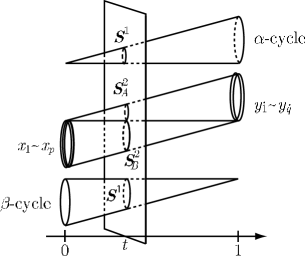
Figure 3: The orbifold is represented as a fibration over the segment $0\leq t\leq 1$.

Due to the ${\bf Z}_{p}\oplus{\bf Z}_{q}$ orbifolding, the periods of $\alpha$ and $\beta$-cycles ara $2\pi/p$ and $2\pi/q$, respectively. If we combine ${\bf S}_{A}^{2}$, ${\bf S}_{B}^{2}$, and the segment parameterized by $t$, they form a $5$-sphere $B={\bf S}^{5}$. We can regard the orbifold $M_{p,q}$ as a ${\bf T}^{2}$ fibration over $B$.

At $t=0$, which defines ${\bf S}^{2}\subset B$, the Lens space $L_{p}$ shrinks and so does the $\alpha$-cycle. Similarly, on ${\bf S}^{2}\subset B$ with $t=1$ the $\beta$-cycle shrinks. These ${\bf S}^{2}$ link to each other in $B$. By blowing up the singularities, these ${\bf S}^{2}$s split into $p$ and $q$ ${\bf S}^{2}$s, respectively. We call them $x_{a}$ ($a=1,\ldots,p$) and $y_{\dot{a}}$ ($\dot{a}=\dot{1},\ldots,\dot{q}$). (Figure 4)

Figure 4: The three segments connecting cycles are examples of three types of three-cycles in the orbifold.

We can follow the IIB/M duality to see that each of them corresponds to the fivebrane with the same index.

$3$-cycles in $M_{p,q}$ can be represented as ${\bf T}^{2}$ fibrations over segments in the base manifold $B={\bf S}^{5}$. There are three types of segments connecting two loci of degenerate fiber. (Figure 4) We denote a segment connecting a point in $x_{a}$ and a point in $x_{b}$ by $[x_{a},x_{b}]$. We similarly define $[y_{\dot{a}},y_{\dot{b}}]$ and $[x_{a},y_{\dot{b}}]$. We also adopt the notation

$$S^{\alpha},S^{\beta},S^{\alpha\beta}\subset M_{p,q}$$ (33)

for the manifold obtained by combining a subset $S\subset B$ and fibers indicated as superscripts. $S^{\alpha\beta}$ is the ${\bf T^{2}}$ fibration over $S$. $S^{\alpha\beta}$ can be regarded as $\beta$-fibration over a certain base manifold, which is isomorphic to $S^{\alpha}$. $S^{\alpha}$ is a global section in this fiber bundle. Therefore, $S^{\alpha}$ can be defined only when $\beta$-cycle fibration over $S$ has a global section. Similarly, we can define $S^{\beta}$ when $\alpha$-cycle fiber has trivial topology over $S$.

With these notations, we can represent $3$-cycles generating $H_{3}$ as

$$[x_{a},x_{b}]^{\alpha\beta},\quad[y_{\dot{a}},y_{\dot{b}}]^{\alpha\beta},\quad[x_{a},y_{\dot{b}}]^{\alpha\beta}.$$ (34)

Because one of $\alpha$ and $\beta$ cycles shrinks at the endpoints of the segments, these are closed $3$-cycles. The topology of $[x_{a},x_{b}]^{\alpha\beta}$ and $[y_{\dot{a}},y_{\dot{b}}]^{\alpha\beta}$ is ${\bf S}^{2}\times{\bf S}^{1}$, and that of $[x_{a},y_{\dot{b}}]^{\alpha\beta}$ is ${\bf S}^{3}$.

These $3$-cycles are not linearly independent. There are combinations of cycles which can be unwrapped. Let us consider

$$\sum_{a=1}^{p}[x_{a},y_{\dot{b}}]^{\alpha\beta}.$$ (35)

This union of $3$-cycles can be unwrapped in $M_{p,q}$. This can be shown by giving a $4$-chain whose boundary is (35). Such an “unwrapping chain” is constructed in the following way. Because $\pi_{2}({\bf S}^{5})=0$, there is a three dimensional disk ${\bf D}^{3}\subset B$ whose boundary is $y_{\dot{b}}$. (The gray disk in Figure 5)

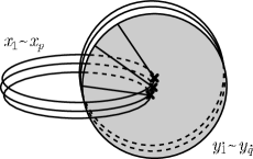
Figure 5: The $\beta$-cycle fibration over the gray disk with the segments removed is an example of unwrapping four-chains.

We call this $Y_{\dot{b}}$. (We also define $X_{a}$ in the same way for $x_{a}$.) This disk intersects once with every $x_{a}$ ($a=1,\ldots,p$). Let $\bar{Y}_{\dot{b}}$ be the subset of $Y_{\dot{b}}$ obtained by removing segments connecting these intersecting points and $y_{\dot{b}}$ (the segments in Fig 5) from the disk.

$$\bar{Y}_{\dot{b}}=Y_{\dot{b}}\backslash\sum_{a=1}^{p}[x_{a},y_{\dot{b}}].$$ (36)

Because $\bar{Y}_{\dot{b}}$ is contractible, we can define $\bar{Y}_{\dot{b}}^{\beta}$. (Note that we cannot define $Y_{\dot{b}}^{\beta}$ because the $\alpha$ cycle is twisted around the intersecting points of $Y_{\dot{b}}$ and $x_{a}$.) We can see that the boundary of the manifold $\bar{Y}_{\dot{b}}^{\beta}$ is

$$\partial\bar{Y}_{\dot{b}}^{\beta}=\sum_{a=1}^{p}[x_{a},y_{\dot{b}}]^{\alpha\beta}.$$ (37)

This may seem at first sight strange because although $\bar{Y}_{\dot{b}}^{\beta}$ does not wrap the $\alpha$-cycle its boundary does. Let us explain this situation by taking Hopf fibration of ${\bf S}^{3}$ as a simple example. By the Hopf fibration ${\bf S}^{3}$ is described as the ${\bf S}^{1}$ fibration over ${\bf S}^{2}$. Let $(\theta,\phi)$ be the polar coordinates of the base ${\bf S}^{2}$. The first Chern class of this fiber bundle is $1$, so that we cannot globally define the coordinate of the fiber. We cover the base ${\bf S}^{2}$ bytwo patches, north patch ($0\leq\theta<\pi$) and south patch ($0<\theta\leq\pi$), and define fiber coordinate $0\leq\psi\leq 2\pi$ separately in each patch. Let $\psi_{N}$ and $\psi_{S}$ be that in north and south patch, respectively. These two coordinats are paseted by the relation $\psi_{N}=\psi_{S}+\phi$. Due to the non-vanishing first Chern class, we cannot take a global section in this fiber bundle. In order to define sections, we need to remove at least one point from the base ${\bf S}^{2}$. Let us take south patch. We can define, for example, the section

$$0<\theta\leq\pi,\quad 0\leq\phi<2\pi,\quad\psi_{S}=0.$$ (38)

At the boundary $\theta=0$ of south patch, the north pole, this section wrap the fiber ${\bf S}^{1}$. This becomes obvious if we use the coordinate $\psi_{N}$, which includes the north pole. The boundary is given by

$$\theta=\pi,\quad 0\leq\phi<2\pi,\quad\psi_{N}=\phi.$$ (39)

This winds once along the fiber ${\bf S}^{1}$. This result makes sense from the fact that the homology $H_{1}({\bf S}^{3})$ vanishes. Any $1$-cycle on ${\bf S}^{3}$ can be unwrapped and represented as the boundary of a $2$-chain.

By exchanging the role of $X_{a}$ and $Y_{\dot{b}}$, we can also show

$$\partial\bar{X}_{a}^{\alpha}=\sum_{\dot{b}=1}^{\dot{q}}[x_{a},y_{\dot{b}}]^{\alpha\beta}.$$ (40)

From (37) and (40), we obtain the homology relation

$$\sum_{a=1}^{p}[x_{a},y_{\dot{b}}]^{\alpha\beta}=\sum_{{\dot{b}}=\dot{1}}^{\dot{q}}[x_{a},y_{\dot{b}}]^{\alpha\beta}=0.$$ (41)

To clarify the relation between the IIB picture and the M-theory picture, we define formal basis ${\bf x}_{a}$ and ${\bf y}_{\dot{b}}$ and rewrite cycles as $[x_{a},x_{b}]^{\alpha\beta}={\bf x}_{a}-{\bf x}_{b}$ and so on. A general superposition of cycles, which is depicted as a junction in $B$, can be written as a linear combination

$${\bf j}=\sum_{a=1}^{p}m_{a}{\bf x}_{a}+\sum_{\dot{a}=\dot{1}}^{\dot{q}}m_{\dot{a}}{\bf y}_{\dot{a}},$$ (42)

where the coefficients must satisfy the constraint (19). We have one to one correspondence between $3$-cycles in $M_{p,q}$ and D3-brane distributions in IIB picture by simply identifying the coefficients in (42) to the components of the charge vector (18). Via this isomorphism the boundaries (37) and (40) correspond to ${\bf w}_{\dot{b}}$ and ${\bf v}_{a}$, the generators of $H$, and the relation (41) defines the homology $H_{3}$ as the same coset group $\Gamma/H$ in (23).

5 Five cycles and baryonic operators

In this section, we discuss the relation between M5-branes wrapped on five cycles and baryonic operators in the ${\cal N}=4$ Chern-Simons theory. In the case of ABJM model, such analysis is done in Park:2008bk, and the conformal dimension and multiplicity of baryonic operators are reproduced on the gravity side. We extend the results to ${\cal N}=4$ Chern-Simons theories.

As in the previous section, we consider $k=1$ case. As is given in (31), the five-cycle homology of $M_{p,q}$ is

$$H_{5}(M_{p,q},{\bf Z})={\bf Z}^{p+q-2},$$ (43)

and when $p+q\geq 3$, there exist non-trivial cycles on which M5-branes can be wrapped. If we represent $M_{p,q}$ as the ${\bf T}^{2}$ fibration over $B={\bf S}^{5}$, the five-cycles can be written as the ${\bf T}^{2}$ fibrations over three-disks.

$$\Omega_{a}:=X_{a}^{\alpha\beta},\quad\Omega_{\dot{a}}:=Y_{\dot{a}}^{\alpha\beta}.$$ (44)

These generate the homology $H_{5}(M_{p,q},{\bf Z})$.

The number of the cycles in (44) is larger than the dimension of $H_{5}(M_{p,q},{\bf Z})$ by two, and there should be two relations among the cycles in (44). Indeed, we have the following homology relations

$$\sum_{a=1}^{p}\Omega_{a}=\sum_{\dot{a}=\dot{1}}^{\dot{q}}\Omega_{\dot{a}}=0.$$ (45)

As we have done in section §4 for three-cycles, we can give these linear combinations as the boundaries of unwrapping $6$-chains. We define a submanifold $\bar{B}\subset B$ by

$$\bar{B}=B\backslash\left(\sum_{a=1}^{p}X_{a}+\sum_{\dot{a}=\dot{1}}^{\dot{p}}Y_{\dot{a}}\right).$$ (46)

If we could draw ${\bf S}^{2}$ enclosing $x_{a}$ in $\bar{B}$, the $\alpha$-cycle fiber would have non-trivial twist on the ${\bf S}^{2}$. However, such ${\bf S}^{2}$ do not exist in $\bar{B}$ because we removed the disks $X_{a}$. Thus the $\alpha$-cycle fiber over $\bar{B}$ has trivial topology and we can define global sections. Similarly, thanks to the removal of $Y_{\dot{a}}$, the $\beta$-cycle fiber also have the trivial topology. Because there is a global section associated with $\alpha$-cycle over $\bar{B}$, the manifold $\bar{B}^{\beta}$ is well-defined, and its boundary is

$$\partial\bar{B}^{\beta}=\sum_{a=1}^{p}X_{a}^{\alpha\beta}.$$ (47)

We also obtain

$$\partial\bar{B}^{\alpha}=\sum_{\dot{a}=1}^{\dot{q}}Y_{\dot{a}}^{\alpha\beta}.$$ (48)

As a result, we obtain the relations (45).

What are the corresponding baryonic operators on the gauge theory side? A natural guess is that these five-cycles are dual to the following operators in the Chern-Simons theory:

$$\Omega_{a} \leftrightarrow B_{a}^{\alpha_{1}\alpha_{2}\cdots\alpha_{N}}=\epsilon_{i_{1}\cdots i_{N}}\epsilon^{j_{1}\cdots j_{N}}h_{a}^{\alpha_{1}}{}^{i_{1}}_{j_{1}}\cdots h_{a}^{\alpha_{N}}{}^{i_{N}}_{j_{N}},$$ (49)

$$\Omega_{\dot{a}} \leftrightarrow B_{\dot{a}}^{\dot{\alpha}_{1}\dot{\alpha}_{2}\cdots\dot{\alpha}_{N}}=\epsilon_{i_{1}\cdots i_{N}}\epsilon^{j_{1}\cdots j_{N}}h_{\dot{a}}^{\dot{\alpha}_{1}}{}^{i_{1}}_{j_{1}}\cdots h_{\dot{a}}^{\dot{\alpha}_{N}}{}^{i_{N}}_{j_{N}}.$$ (50)

Each of these operators is charged under the baryonic symmetry $G_{B}$, and cannot be decomposed into mesonic operators, which are $G_{B}$ neutral. However, the products

$$\prod_{a=1}^{p}B_{a},\quad\prod_{\dot{a}=1}^{\dot{q}}B_{\dot{a}}$$ (51)

carry the same baryonic charge as $e^{iN{\tilde{a}}}$ and $e^{-iN{\tilde{a}}}$, respectively, and by multiplying appropriate power of operator $e^{i{\tilde{a}}}$, we can construct neutral operators with respect to the baryonic symmetries. This strongly suggests that these can be decomposable to the mesonic operators as

$$e^{-iN{\tilde{a}}}\prod_{a=1}^{p}B_{a}\sim b^{N},\quad e^{iN{\tilde{a}}}\prod_{\dot{a}=1}^{\dot{q}}B_{\dot{a}}\sim\tilde{b}^{N}.$$ (52)

This decomposability corresponds to the homology relation (45) among the five cycles.

As a non-trivial check of the duality, let us compare the mass of the wrapped M5-branes and the conformal dimension of the operators. According to the standard AdS/CFT dictionary, the conformal dimension $\Delta$ of an operator and the mass $M$ of the corresponding object are related by $\Delta=R_{{\rm AdS}_{4}}M$. In the case of an M5-brane wrapped on $\Omega_{a}$, this relation becomes

$$\Delta=R_{AdS_{4}}T_{M5}R_{S^{7}}^{5}\mathop{\rm Vol}(\Omega_{a})=\frac{Npq}{2\pi^{3}}\mathop{\rm Vol}(\Omega_{a}).$$ (53)

where $\mathop{\rm Vol}(\Omega_{a})$ is the volume of the 5-cycle $\Omega_{a}$ in $M_{p,q}$ with radius $1$, and to obtain the last expression we used (15) with $k=1$ and the M5-brane tension $T_{M5}=2\pi/(2\pi l_{p})^{6}$. Let us calculate the volume of the 5-cycle. The $5$-cycle $\Omega_{a}$, which is represented as a fiber bundle over the segment $0\leq t\leq 1$, is illustrated as the shaded region in Figure 6.

Figure 6: The shaded region is a nontrivial 5-cycle $X_{a}^{\alpha\beta}$.

The radii of two $3$-spheres defined by (32) are $r_{1}=t^{1/2}$ and $r_{2}=(1-t)^{1/2}$, respectively. The cross-section at $t$ is ${\bf S}^{1}\times{\bf S}^{2}\times{\bf S}^{1}$ with their radii $r_{1}/p$, $r_{2}/2$, $r_{2}/q$, respectively. Hence the volume of the 5-cycle is

$$\mathop{\rm Vol}(\Omega_{a})=\int_{t=0}^{t=1}ds\left(\frac{2\pi r_{1}}{p}\right)\times\left(4\pi\left(\frac{r_{2}}{2}\right)^{2}\right)\times\left(\frac{2\pi r_{2}}{q}\right)=\frac{\pi^{3}}{pq},$$ (54)

where $ds$ is the line element with respect to the parameter $t$ computed as

$$ds^{2}=dr_{1}^{2}+dr_{2}^{2}=\frac{1}{4t(1-t)}dt^{2}.$$ (55)

(The volume (54) is simply $\mathop{\rm Vol}({\bf S}^{5})/pq$ because the five-cycles considered here are orbifolds of large ${\bf S}^{5}$ in ${\bf S}^{7}$.) We obtain the same result for $5$-cycles $Y_{\dot{a}}^{\alpha\beta}$. By substituting this into (53) we obtain

$$\Delta=\frac{1}{2}N,$$ (56)

and this agrees with the conformal dimension of the baryonic operators (49) and (50). (56) is consistent with the result of more general analysis in Yee:2006ba for generic toric tri-Sasakian manifolds.

The degeneracy of the baryonic operators are explained in the same way as the Klebanov-Witten theory [22]. The collective coordinates of five-cycle $\Omega_{a}$ are the coordinates in the transverse direction ${\bf S}^{2}_{A}$, on which $SU(2)_{A}$ acts as rotation. The seven-form flux in the background plays a role of magnetic field on ${\bf S}_{A}^{2}$ and the amount of the flux is $N$. Therefore, the effective theory of the corrective coordinates is the theory of a charged particle in ${\bf S}_{A}^{2}$ with $N$ unit magnetic flux. The ground states of the particle are the $N+1$ states at the lowest Landau level [37] belonging to the spin $N/2$ representation of $SU(2)_{A}$. This degeneracy agrees with that of the baryonic operators $B_{a}$. In the same way, we can explain the degeneracy of $B_{\dot{a}}$ as that of the lowest Landau level of a charged particle in the transverse direction ${\bf S}^{2}_{B}$.

6 Generalization to $k\geq 2$

In this section we generalize the analysis in the previous sections to the case of $k\geq 2$.

Let us first consider fractional D3-brane charges in the type IIB brane setup. We can realize the Chern-Simons theory at level $k$ by replacing D5-branes by $(k,1)$ fivebranes. We can again represent distributions of D3-branes by charge vectors (18) with their components constrained by (19). The only difference from the $k=1$ case is that when a $(k,1)$-brane and an NS5-brane pass through each other, not one but $k$ D3-branes are generated. As a result, the vectors (21) and (22) are multiplied by the extra factor $k$. Namely, we should replace the subgroup $H$ by $kH$ which is generated by $k{\bf v}_{a}$ and $k{\bf w}_{\dot{a}}$, and the quotient group becomes

$$\Gamma/(kH)=(\Gamma/kH^{\prime})/(H/H^{\prime})=({\bf Z}_{kq}^{p-1}\oplus{\bf Z}_{kp}^{q-1}\oplus{\bf Z}_{kpq})/({\bf Z}_{p}\oplus{\bf Z}_{q}).$$ (57)

On the other hand, the homologies $H_{i}(M_{p,q,k},{\bf Z})$ are

$$H_{0}={\bf Z},\quad H_{1}={\bf Z}_{k},\quad H_{2}={\bf Z}^{p+q-2},\quad H_{3}=({\bf Z}_{kp}^{q-1}\oplus{\bf Z}_{kq}^{p-1}\oplus{\bf Z}_{kpq})/({\bf Z}_{p}\oplus{\bf Z}_{q}),$$

$$H_{4}=0,\quad H_{5}={\bf Z}^{p+q-2}\oplus{\bf Z}_{k},\quad H_{6}=0,\quad H_{7}={\bf Z}.$$ (58)

We find that the homology $H_{3}$ is again identical to (57). Let us construct the homology $H_{3}(M_{p,q,k},{\bf Z})$ more explicitly. When the level $k$ is greater than $1$, we have additional ${\bf Z}_{k}$ factor in the orbifold group. As is shown in (7), the generator of ${\bf Z}_{k}$ shifts both $\alpha$ and $\beta$ cycle by $1/k$ of their periods. Because two cycles nowhere shrink at the same time, this action does not generate fixed points. The ${\bf Z}_{k}$ identification in the ${\bf T}^{2}$ fiber generates new cycles, which are not integral linear combinations of $\alpha$ and $\beta$. They are multiples of

$$\gamma=\frac{1}{k}(\alpha-\beta).$$ (59)

As a result, the $2$-cycle defined as the product of $\alpha$ and $\beta$ is not the fundamental ${\bf T}^{2}$ but its multiple $k{\bf T}^{2}$. Thus the cycles (34) are decomposed into $k$ copies of the following elementary cycles.

$$[x_{a},x_{b}]^{\alpha\gamma},\quad[y_{\dot{a}},y_{\dot{b}}]^{\alpha\gamma},\quad[x_{a},y_{\dot{b}}]^{\alpha\gamma}.$$ (60)

Due to this fact, the boundary of unwrapping $4$-chains (40) and (37) are replaced by

$$\partial\bar{X}_{a}^{\alpha}=k(-q{\bf x}_{a}+\sum_{\dot{b}=\dot{1}}^{\dot{q}}{\bf y}_{\dot{b}}),\quad\partial\bar{Y}_{\dot{a}}^{\beta}=k(\sum_{b=1}^{p}{\bf x}_{b}-p{\bf y}_{\dot{a}}),$$ (61)

where we defined the formal basis ${\bf x}_{a}$ and ${\bf y}_{\dot{a}}$ by $[x_{a},x_{b}]^{\alpha\gamma}={\bf x}_{a}-{\bf x}_{b}$ and so on. These precisely correspond to the vectors $k{\bf v}_{a}$ and $k{\bf w}_{\dot{a}}$, and thus the homology $H_{3}$ becomes isomorphic to the quotient $\Gamma/kH$ in (57).

Next, let us consider the relation between baryonic operators and $5$-cycle homology $H_{5}$ for $k\geq 2$. In the case of $k\geq 2$, the generators of the homology in (44) should be replaced by

$$\Omega_{a}=X_{a}^{\alpha\gamma},\quad\Omega_{\dot{a}}=Y_{\dot{a}}^{\alpha\gamma},$$ (62)

and M5-branes wrapped on these generating cycles are identified with the baryonic operators $B_{a}$ and $B_{\dot{a}}$. We can again easily check that the volume of the five-cycles correctly reproduce the conformal dimension $\Delta=N/2$. The $p+q$ generators (62) are not linearly independent, and we can take $\bar{B}^{\alpha}$, $\bar{B}^{\beta}$, and $\bar{B}^{\gamma}$ as unwrapping $6$-chains which give the relation among these generators. Their boundaries are

$$\partial\bar{B}^{\alpha} = \sum_{\dot{a}=\dot{1}}^{\dot{q}}Y_{\dot{a}}^{\alpha\beta}=k\sum_{\dot{a}=\dot{1}}^{\dot{q}}\Omega_{\dot{a}},$$ (63)

$$\partial\bar{B}^{\beta} = \sum_{a=1}^{p}X_{a}^{\alpha\beta}=k\sum_{a=1}^{p}\Omega_{a},$$ (64)

$$\partial\bar{B}^{\gamma} = \sum_{a=1}^{p}X_{a}^{\gamma\beta}+\sum_{\dot{a}=\dot{1}}^{\dot{q}}Y_{\dot{a}}^{\gamma\alpha}=\sum_{a=1}^{p}\Omega_{a}+\sum_{\dot{a}=\dot{1}}^{\dot{q}}\Omega_{\dot{a}}.$$ (65)

Namely, these linear combinations of five-cycles are in trivial element of the homology $H_{5}$. By dividing the group ${\bf Z}^{p+q}$ generated by the $p+q$ basis $\Omega_{a}$ and $\Omega_{\dot{a}}$ by its subgroup ${\bf Z}^{2}$ generated by the above boundaries, we obtain the $H_{5}$ homology in (58).

On the field theory side, the linear dependence of the five-cycles are interpreted as the decomposability of the products of the baryonic operators into the mesonic operators. The first two, (63) and (64), correspond to the product of $B_{a}$ and $B_{\dot{a}}$, respectively, and are decomposed into $N$-th power of operators defined in (12).

$$e^{-iN{\tilde{a}}}\prod_{a=1}^{p}B_{a}^{k}\sim b^{N},\quad e^{iN{\tilde{a}}}\prod_{\dot{a}=1}^{\dot{q}}B_{\dot{a}}^{k}\sim\tilde{b}^{N},$$ (66)

The third boundary (65) corresponds to the product of all the $p+q$ baryonic operators, and it can be decomposed into trace operators.

$$\prod_{a=1}^{p}B_{a}^{k}\prod_{\dot{a}=1}^{\dot{q}}B_{\dot{a}}^{k}\sim\left(\mathop{\rm tr}\nolimits(\prod_{a=1}^{p}h_{a}\prod_{\dot{a}=\dot{1}}^{\dot{q}}h_{\dot{a}})\right)^{N}.$$ (67)

The degeneracy of baryonic operators for $p+q\geq 3$ are again reproduced in the same way as the $k=1$ case. In the case of $p=q=1$ (ABJM model), we need a special treatment because the global symmetry (9) is enhanced to $SU(4)\times U(1)$ and the motion of collective coordinates are treated as a point particle in $SU(4)/(SU(3)\times U(1))$. This is considered in Park:2008bk and the correct multiplicity is obtained.

7 Quark-baryon transition

In §5, we studied the relation between wrapped M5-branes and baryonic operators $B_{I}$. We can relate them more directly by using IIB/M duality explained in §4. By following the duality, we can easily see that an M5-brane wrapped on $\Omega_{I}$ is dual to a D3-brane disk ending on fivebrane $I$, and as we explain below, the D3-brane disk can be continuously deformed to $N$ open strings corresponding to the constituent bi-fundamental quarks. (Similar transition in different brane systems are also considered in Imamura:2006ie,Lee:2006hw.)

Before we explain the deformation, we comment on a relevant fact about flux conservation on the worldvolume of a D3-brane ending on an NS5-brane. The $U(1)$ gauge field $A$ on an NS5-brane electrically couples to endpoints of D-strings on the NS5-brane. This is the case, too, for magnetic flux $f=da$ on D3-branes, which can be regarded as D-strings dissolved in the D3-brane worldvolume. This coupling is described as the action

$$S=\frac{1}{2\pi}\oint_{\partial D3}A\wedge f.$$ (68)

By integrating by part, this is rewritten as

$$S=\frac{1}{2\pi}\oint_{\partial D3}a\wedge F,$$ (69)

and this implies that the flux $F=dA$ on the NS5-brane behaves as an electric charge on the boundary of the D3-brane coupled by the gauge field $a$. If the D3-brane worldvolume is compact, the electric flux conservation requires the total electric charge vanish. If the integral of flux $F$ over the D3-brane boundary is $2\pi N$, we need $N$ strings ending on the D3-brane worldvolume to compensate the boundary charge. This is also the case for a D3-brane ending on a $(k,1)$ fivebrane.

Baring this fact in mind, we can show that $N$ open strings and a D3-brane disk can be continuously deformed to each other. In the following we treat three sets of D3-branes, and for distinction we name them as follows:

• $X$ – the coincident $N$ D3-branes between fivebranes $I$ and $I-1$.

• $Y$ – the coincident $N$ D3-branes between fivebranes $I$ and $I+1$.

• $D$ – a D3-brane disk whose boundary is ${\bf S}^{2}$ on fivebrane $I$.

We here assume that $N_{I}=N_{I-1}=N$. Let us start from a D3-brane disk $D$ whose boundary is ${\bf S}^{2}$ on the fivebrane $I$ enclosing the both boundaries of $X$ and $Y$. ((a) in Figure 7)

Figure 7: Quark-baryon transition

Although these boundaries carry magnetic charges coupled by $A$, their charges cancel each other, and the net flux passing through the boundary $\partial D$ is zero. There are no open strings ending on $D$.

We move the disk so that $\partial Y$, the boundary of $Y$, gets out of $\partial D$. When $\partial Y$ passes through $\partial D$, the flux through $\partial D$ jumps by $N$, and $N$ open strings stretched between $Y$ and $D$ are generated so that the total electric charge on the disk cancels. ((b) in Figure 7)

If we keep moving the disk and $\partial X$ also gets out of the boundary $\partial D$, the flux through the boundary jumps again by $-N$, and this time $N$ open strings stretched between $D$ and $X$ are generated. Two sets of $N$ strings can be connected to get off from $D$, and we obtain $N$ open strings connecting $X$ and $Y$. ((c) in Figure 7) The disk can annihilate without any obstructions.

If $m_{I}=N_{I}-N_{I-1}\neq 0$, the D3-brane disk D in Figure 7 (a) is accompanied by $m_{I}$ strings attached on it. This corresponds to the fact that we cannot define such $SU(N_{I-1})\times SU(N_{I})$ invariant operators as (49) and (50) due to the mismatch of the number of indices. The $m_{I}$ open strings attached on the D3-brane disk corresponds to $m_{I}$ fundamental or $-m_{I}$ anti-fundamental indices which are not contracted.

8 Three-form torsion and fractional branes

In this section, we relate the fractional brane charge and integrals of the $3$-form field on $3$-cycles. Let us consider a process in which the number of the fractional branes changes. The fractional brane charge $Q\in H_{3}$ affects the $3$-form field $C_{3}$ and measured by the integrals over $3$ cycles $\zeta$

$$\oint_{\zeta}C_{3},\quad\zeta\in H_{3}.$$ (70)

We define the period integral at $r=r_{0}$ between the horizon $r=0$ and the AdS boundary $r=\infty$. To change the fractional brane charge by $\Delta Q$, we add an M5-brane wrapped on a $3$-cycle $\Delta Q\in H_{3}$ at the AdS boundary, and move it to the horizon. When the M5-brane pass through $r=r_{0}$, the period integrals changes by

$$\Delta\oint_{\zeta}C_{3}=2\pi\langle\zeta,\Delta Q\rangle,$$ (71)

where $\langle*,*\rangle$ is a map $H_{3}\times H_{3}\rightarrow U(1)$, so called the torsion linking form, or, simply, the linking number.

The linking number is defined as follows. Let $s$ be the order of $\zeta$. Namely, $s$ is the smallest positive integer such that $s\zeta$ is homologically trivial. Such an integer always exists because $H_{3}$ is pure torsion. There exists a $4$-chain $D$ such that

$$s\zeta=\partial D.$$ (72)

We define the linking number $\langle\zeta,\eta\rangle$ of two $3$-cycles $\zeta$ and $\eta$ by

$$\langle\zeta,\eta\rangle=\frac{1}{s}\langle\langle D,\eta\rangle\rangle.$$ (73)

where $\langle\langle D,\eta\rangle\rangle$ is the intersection number of the $4$-chain $C$ and $3$-cycle $\eta$. Because this number jumps by integers by continuous deformations, only the fractional part of the linking number is a topological invariant.

If we move an M5-brane wrapped on the $3$-cycle $\Delta Q$ from the AdS boundary to the horizon, when it passes through $r=r_{0}$, the M5-brane intersect with the $4$-chain $D$ at $\langle\langle D,\eta\rangle\rangle$ points. In this process, the four-form flux $G_{4}$ passing through $D$, including the contribution of Dirac’s string-like objects, changes by $2\pi\langle\langle D,\zeta\rangle\rangle$. By using Stokes’ theorem we obtain the relation (71).

For the manifold $M_{p,q,k}$, following the definition of the linking number, we can easily obtain

$$k\langle{\bf v}_{a},{\bf j}\rangle=m_{a},\quad k\langle{\bf w}_{\dot{a}},{\bf j}\rangle=m_{\dot{a}},$$ (74)

for a general $3$-cycle ${\bf j}$ in (42). The linking numbers among the basis are

$$\langle{\bf x}_{a},{\bf x}_{b}\rangle=-\frac{1}{kq}\delta_{ab},\quad\langle{\bf y}_{\dot{a}},{\bf y}_{\dot{b}}\rangle=-\frac{1}{kp}\delta_{\dot{a}\dot{b}},\quad\langle{\bf x}_{a},{\bf y}_{\dot{b}}\rangle=-\frac{1}{2kpq}.$$ (75)

Due to the constraint (19), the linking number among the basis is not unique. For example, a constant shift of all the linking numbers in (75) does not affect the linking numbers for $3$-cycles which are linear combination of the basis with the coefficient constrained by (19).

By “integrating” the relation (71) and using (74), we obtain

$$m_{a}-m_{a}^{0}=\frac{k}{2\pi}\oint_{{\bf v}_{a}}C_{3},\quad m_{\dot{a}}-m_{\dot{a}}^{0}=\frac{k}{2\pi}\oint_{{\bf w}_{\dot{a}}}C_{3},$$ (76)

where $m_{a}^{0}$ and $m_{\dot{a}}^{0}$ are integration constants which cannot be determined from (71).

Although gauge transformations can change the period integrals of $C_{3}$, the relation (76) determines a element of $\Gamma/kH$ in a gauge invariant way if we know $m_{a}^{0}$ and $m_{\dot{a}}^{0}$ because large gauge transformation change the charge vector by an element of $kH$.

An important fact is that the constants $m_{a}$ and $m_{\dot{a}}$ depend on the frame, the order of fivebranes. The right hand side of the relations (76) are defined on M-theory side, and is independent of the frame, while $m_{a}$ and $m_{\dot{a}}$ on the left hand side change by multiples of $k$ when we change the order of fivebranes. This means that $m_{a}^{0}$ and $m_{\dot{a}}^{0}$ depends on the frame, and we cannot simply set them to be zero.

To obtain some information about the constants, we use branes corresponding to baryonic operators. Remember that in the IIB setup baryonic operators correspond to D3-brane disks ending on fivebranes, and when $m_{I}\neq 0$, they are accompanied by $m_{I}$ open strings.

A similar phenomenon occurs on the M-theory side. If there is non-trivial background $C$-field M5-branes wrapped on five-cycles are accompanied by M2-branes attached on their worldvolume, and by identifying these M2-branes to strings in the IIB setup, we obtain relations between $m_{I}$ and background $C$-field.

Let us consider the flux conservation on M5-branes and how it relates the background $C$-field and M2-branes attached on it. The two-form field $b_{2}$ on M5-branes couples to the field strength $G_{4}$ in the bulk by the coupling

$$S=\frac{1}{2\pi}\int_{M5}b_{2}\wedge G_{4}.$$ (77)

This implies that the flux behaves as charge on M5-branes. On the worldvolume of an M5-brane wrapped on a five-cycle the total charge coupled by $b_{2}$ must cancel due to the flux conservation. This implies that, the cohomology class of the total charge

$$\left[\frac{1}{2\pi}G_{4}-\delta(\partial M2)\right]\in H^{4}(\Omega_{I},{\bf Z})$$ (78)

must be trivial. $\delta(\partial M2)$ is the four-form delta function with support on the boundaries of M2-branes. By the Poincare duality, this is equivalent to

$$[g]=[\partial M2]\in H_{1}(\Omega_{I},{\bf Z}),$$ (79)

where $g$ is the one-cycle Poincare dual to the flux $(2\pi)^{-1}G_{4}$. The homologies $H_{i}(\Omega_{a},{\bf Z})$ in the five-cycle are given by

$$H_{0}={\bf Z},\quad H_{1}={\bf Z}_{k},\quad H_{2}={\bf Z}^{q-1},\quad H_{3}={\bf Z}^{q-1}\oplus{\bf Z}_{k},\quad H_{4}=0,\quad H_{5}={\bf Z}.$$ (80)

The homologies in $\Omega_{\dot{a}}$ are obtained by replacing $q$ in (80) by $p$. Because $H_{1}(\Omega_{I},{\bf Z})={\bf Z}_{k}$ is pure torsion we can rewrite (79) in terms of the linking form $H_{3}\times H_{1}\rightarrow U(1)$ as

$$\frac{1}{2\pi}\oint_{\zeta}C_{3}=\langle\zeta,\partial M2\rangle,$$ (81)

where $\zeta$ is the generator of the torsion subgroup of $H_{3}(\Omega_{I},{\bf Z})$. It is $\zeta={\bf v}_{a}$ for $\Omega_{a}$ and $\zeta={\bf w}_{\dot{a}}$ for $\Omega_{\dot{a}}$. If we identify $m_{I}$ strings ending on a D3-brane disk with a M2-brane wrapped on $m_{I}\gamma$ where $\gamma$ is the generator of $H_{1}(M_{p,q,k},{\bf Z})=H_{1}(\Omega_{I},{\bf Z})$, (81) can be rewritten as

$$m_{a}=\frac{k}{2\pi}\oint_{{\bf v}_{a}}C_{3},\quad m_{\dot{a}}=\frac{k}{2\pi}\oint_{{\bf w}_{\dot{a}}}C_{3}\quad\mathop{\rm mod}\nolimits k.$$ (82)

This means that

$$m_{a}^{0}=m_{\dot{a}}^{0}=0\mathop{\rm mod}\nolimits k.$$ (83)

This fixes only the frame independent part of $m_{a}^{0}$ and $m_{\dot{a}}^{0}$. Although in the $p=q=1$ case this reproduces the result in Aharony:2008gk for ABJM model, this is not sufficient to establish the relation between the fractional brane charge and the $3$-form torsion for $p+q\geq 3$. We leave this problem for future works.

9 Wrapped M2-branes and monopole operators

The correspondence between Kaluza-Klein modes of massless fields in the internal manifold and primary operators in the corresponding boundary CFT is one of most important claim of AdS/CFT correspondence.

Such a correspondence for ABJM model is discussed in Aharony:2008ug,Klebanov:2008vq. For more general ${\cal N}=2$ quiver gauge theories, which describe M2-branes in toric Calabi-Yau $4$-folds, the relation between the holomorphic monomial functions, which are specified by the charges of toric $U(1)$ symmetries, and mesonic operators consisting of bi-fundamental fields, was proposed in Lee:2007kv. In the reference, a simple prescription to establish concrete coresspondence between Kaluza-Klein modes and mesonic operators is given by utilizing brane crystals[39, 52, 53]. When this method was proposed, it had not yet been realized that the quiver gauge theories are actually quiver Chern-Simons theories. After the importance of the existence of Chern-Simons terms was realized, this proposal was confirmed [43, 44, 45] for special kind of brane crystals which can be regarded as “M-theory lift” of brane tilings[46, 47, 48].

In three-dimensional spacetime, local operators in general carry magnetic charges. Such operators are called monopole operators. In the correspondence between primary operators in three-dimensional CFT and Kaluza-Klein modes, monopole operators play an important role. The results in [46, 47, 48] indicate that the set of primary operators corresponding to the supergravity Kaluza-Klein modes includes only a special kind of monopole operators, “diagonal” monopole operators. Diagonal monopole operators carries only the diagonal $U(1)$ magnetic charges, and are constructed by combining dual photon fields and chiral matter fields. The concrete examples of diagonal operators have already apeared in (12). Because the canonical conjugate of the dual photon field is the diagonal $U(1)$ field strength $F_{D}$, the operator $e^{im\tilde{a}}$ shifts the flux $F_{D}$ by $m$.

For a while we consider a generic Abelian quiver ${\cal N}=2$ Chern-Simons theory. We label verices by $a$ and denote the corresponding gauge group by $U(1)_{a}$. Let us consider a monopole operator with magnetic charges $m_{a}\in{\bf Z}$. The diagonal monopole operator $e^{im\tilde{a}}$ carries the same magnetic charge $m_{a}=m$ for all the $U(1)_{a}$ gauge groups. The gauge invariance of the operator requires the Gauss law constraint

$$m_{a}k_{a}+Q_{a}=0,$$ (84)

where $Q_{a}$ is the $U(1)_{a}$ electric charge carried by matter fields included in the monopole operator. This guarantees the invariance of the operator under the gauge symmetry (11). By summing up this over all $a$, we obtain the constraint

$$\sum_{a}m_{a}k_{a}=0.$$ (85)

Therefore, monopole operators are labeled by $n-1$ independent magnetic charges. One of them is the diagonal monopole charge, and corresponds to a certain component of Kaluza-Klein momentum in the internal space (the D-particle charge from the type IIA perspective).

What are the interpretation of the other $n-2$ magnetic charges? It is natural to identify these with the charges of M2-branes wrapped on two-cycles. Let us return to the ${\cal N}=4$ Chern-Simons theory studied in this paper, which is a special case of ${\cal N}=2$ quiver Chern-Simons theories. The two-cycle homology of the corresponding internal space $M_{p,q,k}$ is

$$H_{2}(M_{p,q,k},{\bf Z})={\bf Z}^{p+q-2},$$ (86)

and the Betti number coincides with the number of independent magnetic charges of non-diagonal monopole operatords.

We now explain why we did not impose $G_{B}$ gauge invariance on baryonic operators. First, let us remember the reason why symmetry groups which act on wrapped branes are usually regarded as global symmetries. Consider $AdS_{d+1}$ with the metric

$$ds^{2}=\frac{R^{2}}{z^{2}}((dx^{\mu})^{2}+dz^{2}),\quad\mu=1,\ldots,d,$$ (87)

and let $A_{\nu}(x^{\mu},z)$ be a $U(1)$ gauge field coupling to wrapped branes. We follow Klebanov:1999tb and consider the Euclidian AdS space. $z$ is the radial coordinate such that the AdS boundary is at $z=0$. Let us assume the asymptotic behavior of the vector field as

$$A_{\nu}\propto z^{\Delta}.$$ (88)

For the convergence of the Euclidian action, $\Delta$ must satisfy the inequality

$$\frac{d}{2}-2<\Delta.$$ (89)

With the equation of motion $d*dA=0$ we obtain the asymptotic behavior of the gauge field

$$A_{\nu}(x^{\mu},z)=a_{\nu}(x^{\mu})+z^{d-2}b_{\nu}(x^{\mu}).$$ (90)

On the AdS boundary we need to impose boundary condition which fixes one of $a_{\nu}(x^{\mu})$ and $b_{\nu}(x^{\mu})$. When $d\geq 4$, only the second term in (90) is allowed by (89) and the boundary condition $a_{\nu}(x^{\mu})=0$ must be imposed. Then the gauge field asymptotically vanishes near the boundary, and this is the reason why the symmetry is global in the boundary CFT.

On the other hand, when $d=3$, both terms in (90) satisfy the inequality (89), and we can choose any one of $a_{\nu}(x^{\mu})=0$ (Dirichlet) and $b_{\nu}(x^{\mu})=0$ (Neumann) as the boundary condition. Indeed, these two boundary conditions first appeared in Breitenlohner:1982jf and are used in Witten:2003ya to construct a pair of Chern-Simons theories which are “S-dual” to each other. Let us take the Neumann boundary condition. In this case, the boundary value of the gauge field $a_{\nu}(x^{\mu})=A_{\nu}(x^{\mu},z=0)$ does not vanish, and is dynamical in the sense that it is path integrated. Thus we can regard this as a gauge field in the boundary CFT, and the wrapped branes coupled by $A_{\nu}$ should be cherged objects in the boundary CFT, too. Because the Dirichlet and Neumann boundary conditions are exchanged by the duality transformation of the gauge field, both kinds of operators corresponding to electric and magnetic particles in the AdS₄ cannot be gauge invariant .

In the case of our M-theory background, the gauge fields $A^{i}=A_{\nu}^{i}dx^{\nu}$ coupling to wrapped M5-branes and $\tilde{A}_{i}=A_{i\nu}dx^{\nu}$ coupling to wrapped M2-branes are defined by

$$C_{6}=\sum_{i=1}^{p+q-2}\omega_{i}\wedge A^{i},\quad C_{3}=\sum_{i=1}^{p+q-2}\omega^{i}\wedge\tilde{A}_{i},$$ (91)

where $C_{3}$ and $C_{6}$ are the three- and six-form potential field, which are dual to each other, and $\omega_{i}$ and $\omega^{i}$ are cohomology basis of $H^{5}(M_{p,q,k},{\bf Z})={\bf Z}^{p+q-2}$ and $H_{\rm free}^{2}(M_{p,q,k},{\bf Z})={\bf Z}^{p+q-2}$, respectively. Because $A^{i}$ and $\tilde{A}_{i}$ are electric-magnetic dual to each other, it is impossible to impose the Dirichlet boundary condition on all of them, and consequently some of wrapped branes inevitablly correspond to gauge variant operators. This is the reason why we did not require the baryonic operators to be $G_{B}$ gauge invariant. Although it may be possible to take some S-dual picture in which wrapped M5-branes correspond to gauge invariant operators, then we have to relate wrapped M2-branes to gauge variant operators.

10 Conclusions

In this paper, we investigated some aspects in the gravity dual of ${\cal N}=4$ quiver Chern-Simons theories. One is fractional branes. We confirmed that the group of fractional brane charge, which is obtained by the analysis of Hanany-Witten effect in the type IIB brane configuration, is isomorphic to the homology $H_{3}(M_{p,q,k},{\bf Z})$. We also established the relation between the fractional brane charge and the torsion of the $3$-form field up to the frame dependent constants. In order to determine the constant part, more detailed analysis would be needed.

We also discuss the duality between baryonic operators in the Chern-Simons theory and M5-branes wrapped on five-cycles in $M_{p,q,k}$. We defined baryonic operators which carries $G_{B}$ charges, and found that the homology group $H_{5}(M_{p,q,k},{\bf Z})$ is consistent with the decomposability of products of baryonic operators into mesonic ones on the field theory side. We also found that the conformal dimension of baryonic operators are consistent with the mass of the wrapped M5-branes. The degeneracy of the baryonic operators were explained as the degeneracy of the ground states for the collective motion of the wrapped M5-branes.

We also commented on the relation between non-diagonal monopole operators and wrapped M2-branes. The two-cycle Betti number $b_{2}$ of the internal manifold $M_{p,q,k}$ is found to coincides with the number of independent magnetic charges of non-diagonal monopole operators.

We did not impose the gauge invariance on baryonic operators. In Section 9 we showed that some of wrapped M2-branes and wrapped M5-branes inevitablly correspond to gauge variant operators in the boundary CFT.

There are many questions left which should be studied. The extension of our analysis to more general quiver Chern-Simons theories with smaller supersymmetry is one of them. Moduli spaces of ${\cal N}=2$ supersymmetric quiver Chern-Simons theories are studied in Martelli:2008si,Ueda:2008hx,Imamura:2008qs,Hanany:2008cd. For the class of theories which described by brane tilings [46, 47, 48] (See also Kennaway:2007tq,Yamazaki:2008bt for reviews.) there is a simple prescription to establish the relation between toric data of Calabi-Yau $4$-folds and Chern-Simons gauge theories [43, 44, 45]. It may be interesting to extend our analysis to such a large class of theories.

In general, dual CFT of toric Calabi-Yau $4$-folds cannot be described by brane tilings. In such a case, brane crystals [39, 52, 53] are expected to play an important role. The relation between brane crystals and dual CFT are not fully understood, and the analysis of homologies and wrapped branes may be helpful to obtain some information about dual CFT.

We hope we will return to these subjects in near future.

References

- [1] J. Bagger and N. Lambert, Phys. Rev. D 75, 045020 (2007) [arXiv:hep-th/0611108].
- [2] J. Bagger and N. Lambert, Phys. Rev. D 77, 065008 (2008) [arXiv:0711.0955 [hep-th]].
- [3] J. Bagger and N. Lambert, JHEP 0802, 105 (2008) [arXiv:0712.3738 [hep-th]].
- [4] A. Gustavsson, arXiv:0709.1260 [hep-th].
- [5] A. Gustavsson, JHEP 0804, 083 (2008) [arXiv:0802.3456 [hep-th]].
- [6] N. Lambert and D. Tong, arXiv:0804.1114 [hep-th].
- [7] J. Distler, S. Mukhi, C. Papageorgakis and M. Van Raamsdonk, JHEP 0805, 038 (2008) [arXiv:0804.1256 [hep-th]].
- [8] D. Gaiotto and E. Witten, arXiv:0804.2907 [hep-th].
- [9] K. Hosomichi, K. M. Lee, S. Lee, S. Lee and J. Park, JHEP 0807, 091 (2008) [arXiv:0805.3662 [hep-th]].
- [10] O. Aharony, O. Bergman, D. L. Jafferis and J. Maldacena, arXiv:0806.1218 [hep-th].
- [11] K. Hosomichi, K. M. Lee, S. Lee, S. Lee and J. Park, JHEP 0809, 002 (2008) [arXiv:0806.4977 [hep-th]].
- [12] J. Bagger and N. Lambert, arXiv:0807.0163 [hep-th].
- [13] M. Schnabl and Y. Tachikawa, arXiv:0807.1102 [hep-th].
- [14] Y. Imamura and K. Kimura, Prog. Theor. Phys. 120 (2008) 509, arXiv:0806.3727 [hep-th].
- [15] Y. Imamura and K. Kimura, J. High Energy Phys. 10 (2008) 040, arXiv:0807.2144.
- [16] M. Benna, I. Klebanov, T. Klose and M. Smedback, arXiv:0806.1519 [hep-th].
- [17] S. Terashima and F. Yagi, arXiv:0807.0368 [hep-th].
- [18] D. L. Jafferis and A. Tomasiello, arXiv:0808.0864 [hep-th].
- [19] J. M. Maldacena, Adv. Theor. Math. Phys. 2, 231 (1998) [Int. J. Theor. Phys. 38, 1113 (1999)] [arXiv:hep-th/9711200].
- [20] O. Aharony, O. Bergman and D. L. Jafferis, arXiv:0807.4924 [hep-th].
- [21] C. S. Park, arXiv:0810.1075 [hep-th].
- [22] D. Berenstein, C. P. Herzog and I. R. Klebanov, JHEP 0206, 047 (2002) [arXiv:hep-th/0202150].
- [23] S. S. Gubser and I. R. Klebanov, Phys. Rev. D 58, 125025 (1998) [arXiv:hep-th/9808075].
- [24] I. R. Klebanov and E. Witten, Nucl. Phys. B 536, 199 (1998) [arXiv:hep-th/9807080].
- [25] T. Kitao, K. Ohta and N. Ohta, Nucl. Phys. B 539, 79 (1999) [arXiv:hep-th/9808111].
- [26] O. Bergman, A. Hanany, A. Karch and B. Kol, JHEP 9910, 036 (1999) [arXiv:hep-th/9908075].
- [27] D. Martelli and J. Sparks, arXiv:0808.0912 [hep-th].
- [28] G. W. Moore and N. Seiberg, “Taming The Conformal Zoo,” Phys. Lett. B220 (1989) 422.
- [29] N. Itzhaki, Phys. Rev. D 67, 065008 (2003) [arXiv:hep-th/0211140].
- [30] A. M. Uranga, JHEP 9901, 022 (1999) [arXiv:hep-th/9811004].
- [31] N. Seiberg, Nucl. Phys. B 435, 129 (1995) [arXiv:hep-th/9411149].
- [32] S. Elitzur, A. Giveon and D. Kutasov, Phys. Lett. B 400, 269 (1997) [arXiv:hep-th/9702014].
- [33] A. Giveon and D. Kutasov, arXiv:0808.0360 [hep-th].
- [34] V. Niarchos, JHEP 0811, 001 (2008) [arXiv:0808.2771 [hep-th]].
- [35] A. Hanany and E. Witten, Nucl. Phys. B 492, 152 (1997) [arXiv:hep-th/9611230].
- [36] H. U. Yee, Nucl. Phys. B 774, 232 (2007) [arXiv:hep-th/0612002].
- [37] S. Coleman, gThe Magnetic Monopole Fifty Yearts Later, h in The Unity of Fundamental Interactions, proceedings of the 19th International School of Subnuclear Physics, Erice, Italy, edited by A. Zichichi, Plenum Press (1983).
- [38] Y. Imamura, JHEP 0612, 041 (2006) [arXiv:hep-th/0609163].
- [39] S. Lee, Phys. Rev. D 75, 101901 (2007) [arXiv:hep-th/0610204].
- [40] I. R. Klebanov and E. Witten, Nucl. Phys. B 556, 89 (1999) [arXiv:hep-th/9905104].
- [41] P. Breitenlohner and D. Z. Freedman, Annals Phys. 144, 249 (1982).
- [42] E. Witten, arXiv:hep-th/0307041.
- [43] K. Ueda and M. Yamazaki, arXiv:0808.3768 [hep-th].
- [44] Y. Imamura and K. Kimura, JHEP 0810, 114 (2008) [arXiv:0808.4155 [hep-th]].
- [45] A. Hanany and A. Zaffaroni, arXiv:0808.1244 [hep-th].
- [46] A. Hanany and K. D. Kennaway, “Dimer models and toric diagrams,” arXiv:hep-th/0503149.
- [47] S. Franco, A. Hanany, K. D. Kennaway, D. Vegh and B. Wecht, JHEP 0601 (2006) 096, arXiv:hep-th/0504110.
- [48] S. Franco, A. Hanany, D. Martelli, J. Sparks, D. Vegh and B. Wecht, JHEP 0601 (2006) 128, arXiv:hep-th/0505211.
- [49] K. D. Kennaway, Int. J. Mod. Phys. A 22, 2977 (2007) [arXiv:0706.1660 [hep-th]].
- [50] M. Yamazaki, arXiv:0803.4474 [hep-th].
- [51] I. Klebanov, T. Klose and A. Murugan, arXiv:0809.3773 [hep-th].
- [52] S. Lee, S. Lee and J. Park, JHEP 0705, 004 (2007) [arXiv:hep-th/0702120].
- [53] S. Kim, S. Lee, S. Lee and J. Park, Nucl. Phys. B 797, 340 (2008) [arXiv:0705.3540 [hep-th]].