Casimir Energy of 5D Warped System and Sphere Lattice Regularization

Abstract

Casimir energy is calculated for the 5D electromagnetism and 5D scalar theory in the warped geometry. It is compared with the flat case(arXiv:0801.3064). A new regularization, called sphere lattice regularization, is taken. In the integration over the 5D space, we introduce two boundary curves (IR-surface and UV-surface) based on the minimal area principle. It is a direct realization of the geometrical approach to the renormalization group. The regularized configuration is closed-string like. We do not take the KK-expansion approach. Instead, the position/momentum propagator is exploited, combined with the heat-kernel method. All expressions are closed-form (not KK-expanded form). The generalized P/M propagators are introduced. Rigorous quantities are only treated (non-perturbative treatment). The properly regularized form of Casimir energy, is expressed in a closed form. We numerically evaluate $\Lambda$(4D UV-cutoff), $\omega$(5D bulk curvature, warp parameter) and $T$(extra space IR parameter) dependence of the Casimir energy. We present two new ideas in order to define the 5D QFT: 1) the summation (integral) region over the 5D space is restricted by two minimal surfaces (IR-surface, UV-surface) ; or 2) we introduce a weight function and require the dominant contribution, in the summation, is given by the minimal surface. Based on these, 5D Casimir energy is finitely obtained after the proper renormalization procedure. The warp parameter $\omega$ suffers from the renormalization effect. The IR parameter $T$ does not. In relation to characterizing the dominant path, we classify all paths (minimal surface curves) in AdS₅ space. We examine the meaning of the weight function and finally reach a new definition of the Casimir energy where the 4D momenta( or coordinates) are quantized with the extra coordinate as the Euclidean time (inverse temperature). We comment on the cosmological constant term and present an answer to the problem at the end. Dirac’s large number naturally appears.

Laboratory of Physics, School of Food and Nutritional Sciences, University of Shizuoka
Yada 52-1, Shizuoka 422-8526, Japan

PACS: PACS NO: 04.50.+h, 11.10.Kk, 11.25.Mj, 12.10.-g 11.30.Er, 

Keywords: Warped geometry, position/momentum propagator, heat-kernel, Casimir energy, sphere lattice, Renormalization of boundary parameters, Cosmological constant

1 Introduction

Figure 1: The configuration of the Casimir energy measurement. The radiation cavity bounded by two parallel perfectly-conducting plates separated by $2l$. The plate size is $2L\times 2L$.

In the dawn of the quantum theory, the divergence problem of the specific heat of the radiation cavity was the biggest one (the problem of the blackbody radiation). It is historically so famous that the difficulty was solved by Planck’s idea that the energy is quantized. In other words, the phase space of the photon field dynamics is not continuous but has the "cell" or "lattice" structure with the unit area ($\Delta x\cdot\Delta p$) of the size $2\pi\hbar$ (Planck constant). The radiation energy is composed of two parts, $E_{Cas}$ and $E_{\beta}$:

$$E_{4dEM}=E_{Cas}+E_{\beta}{\quad,}$$

$$E_{Cas}=\sum_{m_{x},m_{y},n\in{\bf Z}}{\tilde{\omega}}_{m_{x}m_{y}n}{\quad,}\quad E_{\beta}=2\sum_{m_{x},m_{y},n\in{\bf Z}}\frac{{\tilde{\omega}}_{m_{x}m_{y}n}}{{\rm e}^{\beta{\tilde{\omega}}_{m_{x}m_{y}n}}-1}{\quad,}$$

$${{\tilde{\omega}}_{m_{x}m_{y}n}}^{2}=(m_{x}\frac{\pi}{L})^{2}+(m_{y}\frac{\pi}{L})^{2}+(n\frac{\pi}{l})^{2}{\quad,}\quad\quad l\ll L{\quad,}$$ (1)

where the parameter $\beta$ is the inverse temperature, $l$ is the separation length between two perfectly-conducting plates, and $L$ is the IR regularization parameter of the plate-size. See Fig.1. The second part $E_{\beta}$ is, essentially, Planck’s radiation formula. The first one $E_{Cas}$ is the vaccuum energy of the radiation field, that is, the Casimir energy. It is a very delicate quantity. The quantity is formally divergent, hence it must be defined with careful regularization. (See App.B). $E_{Cas}/(2L)^{2}$ does depend only on the boudary parameter $l$. The quantity is a quantum effect and , at the same time, depends on the global (macro) parameter $l$.

$$\frac{E_{Cas}}{(2L)^{2}}=\frac{\pi^{2}}{(2l)^{3}}\frac{B_{4}}{4!}=-\frac{\pi^{2}}{720}\frac{1}{(2l)^{3}}{\quad,}\quad B_{4}\mbox{(the fourth Bernoulli number)}=-\frac{1}{30}{\quad,}$$ (2)

In Fig.2, Planck’s radiation spectrum distribution is shown.

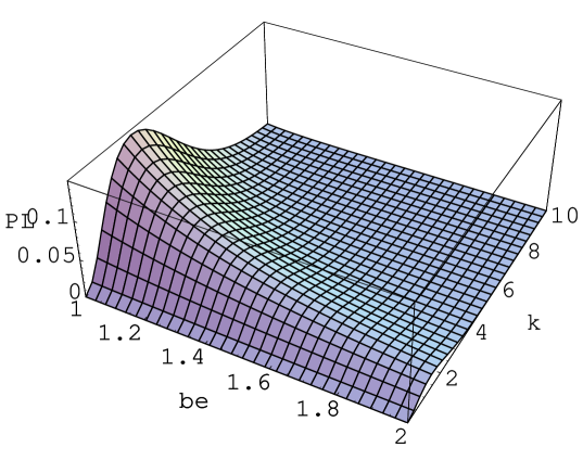
Figure 2: Graph of Planck’s radiation formula. ${\cal P}(\beta,k)=\frac{1}{(c\hbar)^{3}}\frac{1}{\pi^{2}}k^{3}/({\rm e}^{\beta k}-1)\ \ (1\leq\beta\leq 2,\ 0.01\leq k\leq 10),\ \ k\mbox{(photon energy)}=\hbar\omega=h\nu=\hbar c\frac{2\pi}{\lambda},\ \beta=1/k_{B}T$ where $c\hbar=2000\leavevmode\nobreak\ \mbox{eV\leavevmode\nobreak\ \AA},\ k_{B}\mbox{(Boltzmann's constant)}=8.6\times 10^{-5}\leavevmode\nobreak\ \mbox{eV/K}$. $k$=(1,10) eV correspond to $\frac{\lambda}{2\pi}$=(2000,200)Å, $\beta$=(1,2) eV^-1 correspond to T=($10^{5}/8.6,\leavevmode\nobreak\ 10^{5}/17.2$) K. ${\cal P}=0.1$ corresponds to ${\cal P}\Delta k=(2000)^{-3}\times 0.1\times\Delta k$[eV/ų].

Introducing the axis of the inverse temperature($\beta$), besides the photon energy or frequency ($k$), it is shown stereographically. Although we will examine the 5D version of the zero-point part (the Casimir energy), the calculated quantities in this paper are much more related to this Planck’s formula. We see, near the $\beta$-axis, a sharply-rising surface, which is the Rayleigh-Jeans region (the energy density is proportional to the square of the photon frequency). The damping region in high $k$ is the Wien’s region. The ridge (the line of peaks at each $\beta$) forms the hyperbolic curve (Wien’s displacement law). When we will, in this paper, deal with the energy distribution over the 4D momentum and the extra-coordinate, we will see the similar behavior (although top and bottom appear in the opposite way). In order to compare this 4D case with the 5D case of the present paper, we do some preparation for the Casimir energy in App.B.

In the quest for the unified theory, the higher dimensional (HD) approach is a fascinating one from the geometrical point. Historically the initial successful one is the Kaluza-Klein model[2, 3], which unifies the photon, graviton and dilaton from the 5D space-time approach. The HD theories , however, generally have the serious defect as the quantum field theory(QFT) : un-renormalizability. The HD quantum field theories, at present, are not defined within the QFT. One can take the standpoint that the more fundamental formulation, such as the string theory and D-brane theory, can solve the problem. In the present paper, we have the new standpoint that the HD theories should be defined by themselves within the QFT. In order to escape the dimension requirement D=10 or 26 from the quantum consistency (anomaly cancellation)[4], we treat the gravitational (metric) field only as the background one. This does not mean the space-time is not quantized. See later discussions (Sec.7). We present a way to define 5D quantum field theory through the analysis of the Casimir energy of 5D electromagnetism.

In 1983, the Casimir energy in the Kaluza-Klein theory was calculated by Appelquist and Chodos[5]. They took the cut-off ($\Lambda$) regularization and found the quintic ($\Lambda^{5}$) divergence and the finite term. The divergent term shows the unrenormalizability of the 5D theory, but the finite term looks meaningful and, in fact, is widely regarded as the right vacuum energy which shows contraction of the extra axis. In this decade, triggered by the development of the string and D-brane theories, new treatments or new ideas were introduced to calculate the vacuum energy or the effective potential in HD. (The motivation is to settle the stability problem of the moduli parameters[7, 8]. ) One is to regard the system as the bulk and boundary, and do renormalization in both parts[9, 10]. Various regularization methods were carefully re-examined for the bulk-boundary theory[11]. They are applied to various theories including realistic models[12, 13, 14, 15, 16]. From the regularization viewpoint, the zeta-function (or dimensional) regularization combined with some summation formula is most commonly taken. The renormalization procedure, however, does not seem satisfactory. They succeed in calculating the properly regularized quantity and in separating the divergent terms. They found the finite part, but its physical meaning is obscure because the treatment of the divergent part is not established. They simply say, based on the analogy to the case of the ordinary (4D) renormalizable thoeries, the local counterterms can cancel divergences. They try to absorb divergences by the renormalization of parameters such as the brane tension (cosmological constant) and the gravitational constant. But it is fair to say that the $\Lambda^{5}$-divergence problem, posed by Appelquist and Chodos, is not yet solved. All these come from the unsatisfactory situation of the quantum treatment of the brane dynamics and the HD quantum field theories.

In the development of the string and D-brane theories, a new approach to the renormalization group was found. It is called holographic renormalization [17, 18, 19, 20, 21, 22]. We regard the renormalization flow as a curve in the bulk (HD space). The flow goes along the extra axis. The curve is derived as a dynamical equation such as Hamilton-Jacobi equation. It originated from the AdS/CFT correspondence[23, 24, 25]. Spiritually the present basic idea overlaps with this approach. The characteristic points of this paper are: a) We do not rely on the 5D supergravity; b) We do not quantize the gravitational(metric) field; c) The divergence problem is solved by reducing the degree of freedom of the system, where we require, not higher symmetries, but some restriction based on the minimal area principle; d) No local counterterms are necessary.

In the previous paper[26], we investigated the 5D electromagnetism in the flat geometry. For the later use of comparison (with the present warped case), we list the main results here. The extra space is periodic (periodicity $2l$) and $Z_{2}$-parity is taken into account:

$$ds^{2}=\eta_{\mu\nu}dx^{\mu}dx^{\nu}+dy^{2}{\quad,}\quad-\infty<x^{\mu},y<\infty{\quad,}\quad y\rightarrow y+2l,\ y\leftrightarrow-y{\quad,}$$

$$(\eta_{\mu\nu})=\mbox{diag}(-1,1,1,1)\ ,(X^{M})=(X^{\mu}=x^{\mu},X^{5}=y)\equiv(x,y)\ ,$$

$$M,N=0,1,2,3,5;\ \mu,\nu=0,1,2,3.$$ (3)

The IR-regularized geometry of this 5D flat space(-time) is depicted in Fig.3.

Figure 3: IR-regularized geometry of 5D flat space (3). The 4D world (3-brane) is Euclideanized and is shown as 4D ball (shaded disk region) surrounded by $S^{3}$ sphere with radius $\mu^{-1}$. $\mu$ is the 4D IR regularization parameter, and is taken to be $\mu=1/l$. UV-regularization is introduced, in Sec.4, by replacing the 4D ball with the "sphere lattice" composed of many small (size: $1/\Lambda$) 4D balls. See Sec.5 for detail.

The Casimir energy is rigorously (all KK-modes are taken into account) expressed as

$$E_{Cas}(\Lambda,l)=\frac{2\pi^{2}}{(2\pi)^{4}}\int_{1/l}^{\Lambda}d{\tilde{p}}\int_{1/\Lambda}^{l}dy\leavevmode\nobreak\ {\tilde{p}}^{3}W({\tilde{p}},y)F({\tilde{p}},y){\quad,}$$

$$F({\tilde{p}},y)\equiv F^{-}({\tilde{p}},y)+4F^{+}({\tilde{p}},y)=\int_{\tilde{p}}^{\Lambda}d{\tilde{k}}\frac{-3\cosh{\tilde{k}}(2y-l)-5\cosh{\tilde{k}}l}{2\sinh({\tilde{k}}l)}{\quad.}$$ (4)

where $\Lambda$ is the 4D-momentum cutoff, and $W({\tilde{p}},y)$ is the weight function to suppress the IR and UV divergences. We obtained the following $\Lambda$ and $l$ dependence by the numerical analysis.

1) Un-weighted case: $W=1$

$$\mbox{Un-restricted integral region}:\quad\quad\quad\quad\quad\quad\quad$$

$$E_{Cas}(\Lambda,l)=\frac{1}{8\pi^{2}}\left[-0.1249l\Lambda^{5}-(1.41,0.706,0.353)\times 10^{-5}\leavevmode\nobreak\ l\Lambda^{5}\ln(l\Lambda)\right]{\quad,}$$

$$\mbox{Randall-Schwartz integral region}:\quad E^{RS}_{Cas}=\frac{1}{8\pi^{2}}[-0.0894\leavevmode\nobreak\ \Lambda^{4}]{\quad.}$$ (5)

The quintic divergence of the upper one of (5) shows the unrenormalizability of the 5D theory in the ordinary treatment. The triplet data show the unstable situation of numerical results. As for the lower case, the $({\tilde{p}},y)$-integral region is restricted to below the hyperbolic curve ${\tilde{p}}y=1$.

2) Weighted case

$$E^{W}_{Cas}/\Lambda l=\mbox{\hskip 284.52756pt}$$

$$\left\{\begin{array}[]{cc}-2.50\frac{1}{l^{4}}+(-0.142,1.09,1.13)\cdot 10^{-4}\frac{\ln l\Lambda}{l^{4}}&\mbox{for}\quad W=\frac{1}{N_{1}}{\rm e}^{-(1/2)l^{2}{\tilde{p}}^{2}-(1/2)y^{2}/l^{2}}\equiv W_{1}\\ -6.04\leavevmode\nobreak\ 10^{-2}\frac{1}{l^{4}}-(24.7,2.79,1.60)\cdot 10^{-8}\frac{\ln l\Lambda}{l^{4}}&\mbox{for}\quad W=\frac{1}{N_{2}}{\rm e}^{-{\tilde{p}}y}\equiv W_{2}\\ -2.51\frac{1}{l^{4}}+(19.5,11.6,6.68)\cdot 10^{-4}\frac{\ln l\Lambda}{l^{4}}&\mbox{for}\quad W=\frac{1}{N_{8}}{\rm e}^{-(l^{2}/2)({\tilde{p}}^{2}+1/y^{2})}\equiv W_{8}\end{array}\right.$$ (9)

where some representative cases ($W_{1}$: elliptic, $N_{1}=1.557/8\pi^{2}$ ; $W_{2}$: hyperbolic, $N_{2}=2(l\Lambda)^{3}/8\pi^{2}$; $W_{8}$: reciprocal, $N_{8}=0.3800/8\pi^{2}$) are shown. (See ref.[26] for other cases. ) The quantity $\Lambda l$ is the normalization factor in the numerical analysis. The Casimir energy behavior of the case $W_{2}$ is consistent with the Randall-Schwartz’s one of 1). These results imply the renormalization of the compactification size $l$.

$$E^{W}_{Cas}/\Lambda l=-\frac{\alpha}{l^{4}}\left(1-4c\ln(l\Lambda)\right)=-\frac{\alpha}{{l^{\prime}}^{4}}{\quad,}\quad\beta=\frac{\partial}{\partial(\ln\Lambda)}\ln\frac{l^{\prime}}{l}=c{\quad,}$$ (10)

where $\alpha$ and $c$ should be uniquely fixed by clarifying the meaning of the weight function $W$ and the unstable situation of the triplet data.

The aim of this paper is to examine how the above results change for the 5D warped geometry case. The IR-regularized geometry of the 5D warped space(-time) is depicted in Fig.4. One additional massive parameter, that is, the warp (bulk curvature) parameter $\omega$ appears. The limit $\omega\rightarrow 0$ leads to the flat case. This introduction of the "thickness" $1/\omega$ comes from the expectation that it softens the UV-singularity, which is the same situation as in the string theory. See Ref.[27] and [28] besides this work.

Figure 4: IR-regularized geometry of 5D warped space (16). The 4D world (3-brane) is Euclideanized and is shown as a 4D ball (shaded disk region) surrounded by $S^{3}$ sphere with radius $\mu^{-1}$. $\mu$ is the 4D IR regularization parameter. UV-regularization is introduced by replacing the 4D ball with the "sphere lattice" composed of many small (size: $1/\Lambda$) 4D balls. See Sec.5 for detail.

The content is organized as follows. We start with the familiar approach to the 5D warped system: the Kaluza-Klein expansion, in Sec.2. In Sec.3, the same content of Sec.2 is dealt in the heat-kernel method and the Casimir energy is expressed in a closed form in terms of the P/M propagator. The closed expression of Casimir energy enables us numerically evaluate the quantity in Sec.4. Here we introduce UV and IR regularization parameters in (4D momentum, extra coordinate)-space. A new idea about the UV and IR regularization is presented in Sec.5. The minimal area principle is introduced. The sphere lattice and the renormalization flow are explained. In Sec.6 an improved regularization procedure is presented where a weight function is introduced. Here again the minimal surface principle is taken. The meaning of the weight function is given in Sec.7. In Sec.8 we make the concluding remarks. Renormalization of the warp parameter $\omega$ is explicitly shown. We argue the (4D) coordinates or momenta look quantized in the present treatment. The cosmological constant is addressed. We prepare five appendices to supplement the text. App.A deals with the classification of all minimal surface curves in the 5D warped space. App.B reviews 4D Casimir energy (the ordinary radiation cavity problem) where the features of the cut-off and zeta-function regularizations are examined. App.C explains the numerical confirmation of the (approximate) equality of the minimal surface curve and the dominant path in the Casimir energy calculation. The results, appearing in this paper, heavily relies on some numerical calculations. We explain them in App.D. Normalization constants of various weight functions are explained in App.E.

2 Kaluza-Klein expansion approach

In order to analyze the 5D EM-theory, we start with 5D massive vector theory.

$$S_{5dV}={\int d^{4}xdz}\sqrt{-G}(-\frac{1}{4}F_{MN}F^{MN}-{\frac{1}{2}}m^{2}A^{M}A_{M})\ ,\ F_{MN}=\partial_{M}A_{N}-\partial_{N}A_{M}\ ,$$

$$ds^{2}=\frac{1}{\omega^{2}z^{2}}(\eta_{\mu\nu}dx^{\mu}dx^{\nu}+{dz}^{2})=G_{MN}dX^{M}dX^{N}{\quad,}\quad G\equiv\det G_{AB}{\quad,}$$

$$(X^{M})=(x^{\mu},z){\quad,}\quad M,N=0,1,2,3,5(\mbox{or }z);\ \mu,\nu=0,1,2,3{\quad.}$$ (11)

The 5D vector mass, $m$, is regarded as a IR-regularization parameter. In the limit, $m=0$, the above one has the 5D local-gauge symmetry. Casimir energy is given by some integral where the (modified) Bessel functions, with the index $\nu=\sqrt{1+\frac{m^{2}}{\omega^{2}}}$, appear. (See, for example, ref.[29].) Hence the 5D EM limit is given by $\nu=1\ (m=0)$. We consider, however, the imaginary mass case $m=i\omega\ (m^{2}=-\omega^{2},\ \nu=0)$ for the following reasons: 1) the UV-behavior does not depend on the bulk mass parameter m which is regarded as a IR regularization one; 2) we can compare the result with the 5D flat case where the 5D scalars (4 even-parity modes + 1 odd-parity mode) are considered[26], 3) $\nu=0$ Bessel functions are meaningfully simple in the analysis. We can simplify the model furthermore. Instead of analyzing the $m^{2}=-\omega^{2}$ of the massive vector (11), we take the 5D massive scalar theory on AdS₅ with $m^{2}=-4\omega^{2},\ \nu=\sqrt{4+m^{2}/\omega^{2}}=0$.

$${\cal L}=\sqrt{-G}(-{\frac{1}{2}}\nabla^{M}\Phi\nabla_{M}\Phi-{\frac{1}{2}}m^{2}\Phi^{2}){\quad,}\quad G\equiv\det G_{MN}{\quad,}$$

$$ds^{2}=G_{MN}dX^{M}dX^{N}{\quad,}\quad\nabla^{M}\nabla_{M}\Phi-m^{2}\Phi+J=0{\quad,}$$ (12)

where $\Phi(X)=\Phi(x^{\mu},z)$ is the 5D scalar field. The background geometry is AdS₅ which takes the following form, in terms of $z$,

$$(G_{MN})=\left(\begin{array}[]{ll}\frac{1}{\omega^{2}z^{2}}\eta_{{\mu\nu}}&0\\ 0&\frac{1}{\omega^{2}z^{2}}\end{array}\right){\quad,}\quad\sqrt{-G}=\frac{1}{(\omega|z|)^{5}}{\quad,}$$ (15)

$$-\frac{1}{T}\leq z\leq-\frac{1}{\omega}\quad\mbox{or}\quad\frac{1}{\omega}\leq z\leq\frac{1}{T}\quad(-l\leq y\leq l\ ,\ |z|=\frac{1}{\omega}{\rm e}^{\omega|y|}){\quad,}$$

$$\frac{1}{T}\equiv\frac{1}{\omega}{\rm e}^{\omega l}{\quad,}$$ (16)

where we take into account $Z_{2}$ symmetry: $z\leftrightarrow-z$. $\omega$ is the bulk curvature (AdS₅ parameter) and $T^{-1}$ is the size of the extra space (Infrared parameter).

In this section, we do the standard analysis of the warped system, that is, the Kaluza-Klein expansion approach.

The Casimir energy $E_{Cas}$ is given by

$${\rm e}^{-T^{-4}E_{Cas}}=\int{\cal D}\Phi\exp\{i\int d^{5}X{\cal L}\}$$

$$=\int{\cal D}\Phi(X)\exp\left[i{\int d^{4}x}dz\frac{1}{(\omega|z|)^{5}}{\frac{1}{2}}\Phi\{\omega^{2}z^{2}\partial_{a}\partial^{a}\Phi+(\omega|z|)^{5}\frac{\partial}{\partial z}\frac{1}{(\omega z)^{3}}\partial_{z}\Phi-m^{2}\Phi\}\right]{\quad.}$$ (17)

Here we introduce, instead of $\Phi(X)$, the partially (4D world only) Fourier transformed field $\Phi_{p}(z)$.

$$\Phi(X)={\int\frac{d^{4}p}{(2\pi)^{4}}}{\rm e}^{ipx}\Phi_{p}(z){\quad,}$$ (18)

Eq.(17) can be rewritten as

$${\rm e}^{-T^{-4}E_{Cas}}=\int{\cal D}\Phi_{p}(z)\times$$

$$\exp\left[i{\int\frac{d^{4}p}{(2\pi)^{4}}}2\int_{1/\omega}^{1/T}dz\left\{{\frac{1}{2}}\Phi_{p}(z)\{-\frac{1}{(\omega z)^{3}}p^{2}+\frac{d}{dz}\frac{1}{(\omega z)^{3}}\frac{d}{dz}-\frac{m^{2}}{(\omega z)^{5}}\}\Phi_{p}(z)\right\}\right]{\quad,}$$ (19)

where we have used the $Z_{2}$-property, defined in (21), of $\Phi_{p}(z)$. From the above expression, we can read the measure function $s(z)$ and the extra-space kinetic operator ${\hat{L}}_{z}$.

$$s(z)=\frac{1}{(\omega z)^{3}}{\quad,}\quad{\hat{L}}_{z}\equiv\frac{d}{dz}\frac{1}{(\omega z)^{3}}\frac{d}{dz}-\frac{m^{2}}{(\omega z)^{5}}{\quad,}$$ (20)

and consider the Bessel eigen-value problem.

$$\{s(z)^{-1}{\hat{L}}_{z}+{M_{n}}^{2}\}\psi_{n}(z)=0{\quad,}$$

$$\psi_{n}(z)=-\psi_{n}(-z)\quad\mbox{for}\quad P=-\quad;\quad\psi_{n}(z)=\psi_{n}(-z)\quad\mbox{for}\quad P=+{\quad,}$$ (21)

with the appropriate b.c. at fixed points. Because the set $\{\psi_{n}(z)\}$ constitute the orthonormal and complete system, we can express $\Phi_{p}(z)$ as

$$\Phi_{p}(z)=\sum_{n}c_{n}(p)\psi_{n}(z){\quad.}$$ (22)

Eq.(19) can be further rewritten as

$${\rm e}^{-T^{-4}E_{Cas}}=\int{\cal D}\Phi_{p}(z)\exp\left[i{\int\frac{d^{4}p}{(2\pi)^{4}}}2\int_{1/\omega}^{1/T}dz\left\{{\frac{1}{2}}\Phi_{p}(z)s(z)({s(z)}^{-1}{\hat{L}}_{z}-p^{2})\Phi_{p}(z)\right\}\right]$$

$$=\int\prod_{n}dc_{n}(p)\exp\left[{\int\frac{d^{4}p_{E}}{(2\pi)^{4}}}\sum_{n}\{-{\frac{1}{2}}c_{n}(p)^{2}(p_{E}^{2}+M_{n}^{2})\}\right]$$

$$=\exp\sum_{n,p}\{-{\frac{1}{2}}\ln(p_{E}^{2}+M_{n}^{2})\}{\quad,}$$ (23)

where the orthonormal relation

$$2\int_{\frac{1}{\omega}}^{\frac{1}{T}}\psi_{n}(z)s(z)\psi_{m}(z)dz=\delta_{nm}{\quad,}$$ (24)

is used. This shows that $s(z)$, defined in (20), plays the role of "inner product measure" in the function space $\{\psi_{n}(z),1/\omega\leq z\leq 1/T\}$. In (23), Wick’s rotation is done for the time-component of $\{p^{\mu}\}$.

$$ip^{0}\quad\rightarrow\quad p^{4}{\quad,}$$

$$idp^{0}dp^{1}dp^{2}dp^{3}\quad\rightarrow\quad dp^{4}dp^{1}dp^{2}dp^{3}\equiv d^{4}p_{E}{\quad,}$$

$$p^{2}=-(p^{0})^{2}+(p^{1})^{2}+(p^{2})^{2}+(p^{3})^{2}\quad\rightarrow\quad(p^{4})^{2}+(p^{1})^{2}+(p^{2})^{2}+(p^{3})^{2}\equiv p_{E}^{2}{\quad,}$$ (25)

The expression (23) is the familiar one of the Casimir energy.

3 Heat-Kernel Approach and Position/Momentum Propagator

Eq.(23) is the expression of $E_{Cas}$ by the KK-expansion. In this section, the same quantity is re-expressed in a closed form using the heat-kernel method and the P/M propagator.

$${\rm e}^{-T^{-4}E_{Cas}}=\int{\cal D}\Phi_{p}(z)\exp\left[i{\int\frac{d^{4}p}{(2\pi)^{4}}}2\int_{1/\omega}^{1/T}dz\left\{{\frac{1}{2}}\Phi_{p}(z)s(z)({s(z)}^{-1}{\hat{L}}_{z}-p^{2})\Phi_{p}(z)\right\}\right]$$

$$=\exp\left[T^{-3}{\int\frac{d^{4}p_{E}}{(2\pi)^{4}}}2\int_{1/\omega}^{1/T}dzs(z)\left\{-{\frac{1}{2}}\ln(-{s(z)}^{-1}{\hat{L}}_{z}+p_{E}^{2})\right\}\right]$$

$$=\exp\left[T^{-3}{\int\frac{d^{4}p_{E}}{(2\pi)^{4}}}2\int_{1/\omega}^{1/T}dzs(z)\left\{{\frac{1}{2}}\int_{0}^{\infty}\frac{1}{t}{\rm e}^{t({s(z)}^{-1}{\hat{L}}_{z}-p_{E}^{2})}dt+\mbox{const}\right\}\right]$$

$${\quad,}$$ (26)

where we have used a formula[30].

$$\int_{0}^{\infty}\frac{{\rm e}^{-t}-{\rm e}^{-tM}}{t}dt=\ln M{\quad,}\quad\mbox{det}\leavevmode\nobreak\ M>0{\quad,}\quad M\ :\ \mbox{a matrix}{\quad.}$$ (27)

(The factors $T^{-4}$ and $T^{-3}$ in (26) come from the dimensional analysis. $T$ has the meaning of the renormalization point. ) The above formal result can be precisely defined using the heat equation.

$${\rm e}^{-T^{-4}E_{Cas}}=(\mbox{const})\times\exp\left[T^{-4}{\int\frac{d^{4}p_{E}}{(2\pi)^{4}}}2\int_{0}^{\infty}{\frac{1}{2}}\frac{dt}{t}\mbox{Tr}\leavevmode\nobreak\ H_{p_{E}}(z,z^{\prime};t)\right]{\quad,}$$

$$\mbox{Tr}\leavevmode\nobreak\ H_{p}(z,z^{\prime};t)=\int_{1/\omega}^{1/T}s(z)H_{p}(z,z;t)dz{\quad,}\quad\{\frac{\partial}{\partial t}-(s^{-1}{\hat{L}}_{z}-p^{2})\}H_{p}(z,z^{\prime};t)=0{\quad.}$$ (28)

The heat kernel $H_{p}(z,z^{\prime};t)$ is formally solved, using the Dirac’s bra and ket vectors $(z|,|z)$, as

$$H_{p}(z,z^{\prime};t)=(z|{\rm e}^{-(-s^{-1}{\hat{L}}_{z}+p^{2})t}|z^{\prime}){\quad.}$$ (29)

(The bra and ket vectors $(z|,|z)$ are precisely defined by the orthonormal and complete set of ${\hat{L}}_{z}$: $\{\psi_{n}(z)\}$. ) Using the set $\{\psi_{n}(z)\}$ defined in (21), the explicit solution of (28) is given by

$$H_{p}(z,z^{\prime};t)=\sum_{n\in{\bf Z}}{\rm e}^{-(M_{n}^{2}+p^{2})t}{\frac{1}{2}}\{\psi_{n}(z)\psi_{n}(z^{\prime})-\psi_{n}(z)\psi_{n}(-z^{\prime})\}{\quad,}\quad P=-{\quad,}$$

$$E_{p}(z,z^{\prime};t)=\sum_{n\in{\bf Z}}{\rm e}^{-(M_{n}^{2}+p^{2})t}{\frac{1}{2}}\{\psi_{n}(z)\psi_{n}(z^{\prime})+\psi_{n}(z)\psi_{n}(-z^{\prime})\}{\quad,}\quad P=+{\quad,}$$ (34)

where we have used the dimensionality of $H_{p}$ and $E_{p}$ read from (28). ([$E_{p}$]=[$H_{p}$]=$L^{-1}$).

The above heat-kernels satisfy the following b.c..

$$\lim_{t\rightarrow+0}H_{p}(z,z^{\prime};t)=\sum_{n\in{\bf Z}}{\frac{1}{2}}\{\psi_{n}(z)\psi_{n}(z^{\prime})-\psi_{n}(z)\psi_{n}(-z^{\prime})\}\equiv(\omega|z|)^{3}\epsilon(z)\epsilon(z^{\prime}){\hat{\delta}}(|z|-|z^{\prime}|)\ ,\ P=-\ ,$$

$$\lim_{t\rightarrow+0}E_{p}(z,z^{\prime};t)=\sum_{n\in{\bf Z}}{\frac{1}{2}}\{\psi_{n}(z)\psi_{n}(z^{\prime})+\psi_{n}(z)\psi_{n}(-z^{\prime})\}\equiv(\omega|z|)^{3}{\hat{\delta}}(|z|-|z^{\prime}|)\ ,\ P=+\ {\quad,}$$ (35)

where $\epsilon(z)$ is the sign function. The above equation defines ${\hat{\delta}}(|z|-|z^{\prime}|)$. We here introduce the position/momentum propagators $G^{\mp}_{p}$ as follows.

$$G^{-}_{p}(z,z^{\prime})\equiv\int_{0}^{\infty}dt\leavevmode\nobreak\ H_{p}(z,z^{\prime};t)=\sum_{n\in{\bf Z}}\frac{1}{M_{n}^{2}+p^{2}}{\frac{1}{2}}\{\psi_{n}(z)\psi_{n}(z^{\prime})-\psi_{n}(z)\psi_{n}(-z^{\prime})\}{\quad,}$$

$$G^{+}_{p}(z,z^{\prime})\equiv\int_{0}^{\infty}dt\leavevmode\nobreak\ E_{p}(z,z^{\prime};t)=\sum_{n\in{\bf Z}}\frac{1}{M_{n}^{2}+p^{2}}{\frac{1}{2}}\{\psi_{n}(z)\psi_{n}(z^{\prime})+\psi_{n}(z)\psi_{n}(-z^{\prime})\}{\quad.}$$ (36)

They satisfy the following differential equations of propagators.

$$({\hat{L}}_{z}-p^{2}s(z))G^{\mp}_{p}(z,z^{\prime})=\sum_{n\in{\bf Z}}{\frac{1}{2}}\{\psi_{n}(z)\psi_{n}(z^{\prime})\mp\psi_{n}(z)\psi_{n}(-z^{\prime})\}$$

$$=\left\{\begin{array}[]{ll}\epsilon(z)\epsilon(z^{\prime}){\hat{\delta}}(|z|-|z^{\prime}|)&\mbox{for\ \ P=}-1\\ {\hat{\delta}}(|z|-|z^{\prime}|)&\mbox{for\ \ P=}1\end{array}\right.$$ (39)

Therefore the Casimir energy $E_{Cas}$ is, from (28) and (34), given by

$$-E^{-}_{Cas}(\omega,T)={\int\frac{d^{4}p_{E}}{(2\pi)^{4}}}2{\int_{0}^{\infty}\frac{dt}{t}}2\int_{1/\omega}^{1/T}dz\leavevmode\nobreak\ s(z)H_{p_{E}}(z,z;t)$$

$$={\int\frac{d^{4}p_{E}}{(2\pi)^{4}}}2{\int_{0}^{\infty}\frac{dt}{t}}2\int_{1/\omega}^{1/T}dz\leavevmode\nobreak\ s(z)\left\{\sum_{n\in{\bf Z}}{\rm e}^{-(M_{n}^{2}+p_{E}^{2})t}\psi_{n}(z)^{2}\right\}{\quad,}$$ (40)

where $s(z)=1/(\omega z)^{3}$ (20). This expression leads to the same treatment as the previous section. Note that the above expression shows the negative definiteness of $E^{-}_{Cas}$.

Here we introduce the generalized P/M propagators, $I_{\alpha}$(P=$-$) and $J_{\alpha}$(P=+) as

$$I_{\alpha}(p^{2};z,z^{\prime})\equiv\int_{0}^{\infty}\frac{dt}{t^{\alpha}}H_{p}(z,z^{\prime};t)$$

$$=\int_{0}^{\infty}\frac{dt}{t^{\alpha}}\sum_{n\in{\bf Z}}{\rm e}^{-(M_{n}^{2}+p^{2})t}{\frac{1}{2}}\{\psi_{n}(z)\psi_{n}(z^{\prime})-\psi_{n}(z)\psi_{n}(-z^{\prime})\}{\quad,}\quad\mbox{P=}-{\quad,}$$

$$J_{\alpha}(p^{2};z,z^{\prime})\equiv\int_{0}^{\infty}\frac{dt}{t^{\alpha}}E_{p}(z,z^{\prime};t)$$

$$=\int_{0}^{\infty}\frac{dt}{t^{\alpha}}\sum_{n\in{\bf Z}}{\rm e}^{-(M_{n}^{2}+p^{2})t}{\frac{1}{2}}\{\psi_{n}(z)\psi_{n}(z^{\prime})+\psi_{n}(z)\psi_{n}(-z^{\prime})\}{\quad,}\quad\mbox{P=}+{\quad,}$$ (41)

where $\alpha$ is the arbitrary real number. Then we have the following relations.

$$I_{0}(p^{2};z,z^{\prime})=G_{p}^{-}(z,z^{\prime}){\quad,}\quad J_{0}(p^{2};z,z^{\prime})=G_{p}^{+}(z,z^{\prime}){\quad,}$$

$$\frac{\partial I_{\alpha}(p^{2};z,z^{\prime})}{\partial p^{2}}=-I_{\alpha-1}(p^{2};z,z^{\prime}){\quad,}\quad\int_{p^{2}}^{\infty}dk^{2}I_{\alpha}(k^{2};z,z^{\prime})=I_{\alpha+1}(p^{2};z,z^{\prime}){\quad,}$$

$$\frac{\partial J_{\alpha}(p^{2};z,z^{\prime})}{\partial p^{2}}=-J_{\alpha-1}(p^{2};z,z^{\prime}){\quad,}\quad\int_{p^{2}}^{\infty}dk^{2}J_{\alpha}(k^{2};z,z^{\prime})=J_{\alpha+1}(p^{2};z,z^{\prime}){\quad,}$$

$$(p^{2}-r(z)^{-1}{\hat{L}}_{z})I_{\beta}(p^{2};z,z^{\prime})=-\beta I_{\beta+1}(p^{2};z,z^{\prime})\ ,\ (p^{2}-r(z)^{-1}{\hat{L}}_{z})J_{\beta}(p^{2};z,z^{\prime})=-\beta J_{\beta+1}(p^{2};z,z^{\prime})\ ,$$

$$\beta\neq 0{\quad,}$$

$$\frac{\partial I_{\alpha}(p^{2};z,z^{\prime})}{\partial\alpha}=-\int_{0}^{\infty}\frac{\ln t}{t^{\alpha}}dtH_{p}(z,z^{\prime};t){\quad.}$$ (42)

Finally we obtain the following useful expression of the Casimir energy for $P=\mp$.

$$-E^{-}_{Cas}(\omega,T)={\int\frac{d^{4}p_{E}}{(2\pi)^{4}}}\{\mbox{Tr}\leavevmode\nobreak\ I_{1}(p_{E}^{2};z,z^{\prime})\}={\int\frac{d^{4}p_{E}}{(2\pi)^{4}}}\int_{p_{E}^{2}}^{\infty}\{{\rm Tr\,}I_{0}(k^{2};z,z^{\prime})\}dk^{2}$$

$$={\int\frac{d^{4}p_{E}}{(2\pi)^{4}}}\int_{p_{E}^{2}}^{\infty}\{{\rm Tr\,}G_{k}^{-}(z,z^{\prime})\}dk^{2}={\int\frac{d^{4}p_{E}}{(2\pi)^{4}}}\int_{1/\omega}^{1/T}dz\leavevmode\nobreak\ s(z)\int_{p_{E}^{2}}^{\infty}\{G_{k}^{-}(z,z)\}dk^{2}{\quad,}$$

$$-E^{+}_{Cas}(\omega,T)={\int\frac{d^{4}p_{E}}{(2\pi)^{4}}}\{\mbox{Tr}\leavevmode\nobreak\ J_{1}(p_{E}^{2};z,z^{\prime})\}={\int\frac{d^{4}p_{E}}{(2\pi)^{4}}}\int_{p_{E}^{2}}^{\infty}\{{\rm Tr\,}J_{0}(k^{2};z,z^{\prime})\}dk^{2}$$

$$={\int\frac{d^{4}p_{E}}{(2\pi)^{4}}}\int_{p_{E}^{2}}^{\infty}\{{\rm Tr\,}G_{k}^{+}(z,z^{\prime})\}dk^{2}={\int\frac{d^{4}p_{E}}{(2\pi)^{4}}}\int_{1/\omega}^{1/T}dz\leavevmode\nobreak\ s(z)\int_{p_{E}^{2}}^{\infty}\{G_{k}^{+}(z,z)\}dk^{2}{\quad.}$$ (43)

Here we list the dimensions of various quantities appeared above.

$$\begin{array}[]{c|c|c|c|c|c|c|c|c|c}L^{1-2\alpha}&L^{-4}&L^{-3/2}&L^{-1}&L^{-1/2}&L^{0}&L&L^{2}&L^{5/2}&L^{3}\\ \hline\cr&E_{Cas}&&\Lambda,p,\omega,T&&&z,l&t&&\\ I_{\alpha},J_{\alpha}&&&H_{p},E_{p}&&&G^{\mp}_{p}&&&\\ &&\Phi&&&s(z)&&&\Phi_{p}&\\ &&&{\hat{\delta}}(z-z^{\prime})&|z),(z|,\psi_{n}(z)&|n),(n|&&&&c_{n}(p)\end{array}$$

($\Lambda$ is a regularization parameter defined below.)

The P/M propagators $G_{p}^{\mp}$ in (36), (42) and (43) can be expressed in a closed form. (See, for example, [31].) Taking the Dirichlet condition at all fixed points, the expression for the fundamental region ($1/\omega\leq z\leq z^{\prime}\leq 1/T$) is given by

$$G_{p}^{\mp}(z,z^{\prime})=\mp\frac{\omega^{3}}{2}z^{2}{z^{\prime}}^{2}\frac{\{{\bf I}_{0}(\frac{{\tilde{p}}}{\omega}){\bf K}_{0}({\tilde{p}}z)\mp{\bf K}_{0}(\frac{{\tilde{p}}}{\omega}){\bf I}_{0}({\tilde{p}}z)\}\{{\bf I}_{0}(\frac{{\tilde{p}}}{T}){\bf K}_{0}({\tilde{p}}z^{\prime})\mp{\bf K}_{0}(\frac{{\tilde{p}}}{T}){\bf I}_{0}({\tilde{p}}z^{\prime})\}}{{\bf I}_{0}(\frac{{\tilde{p}}}{T}){\bf K}_{0}(\frac{{\tilde{p}}}{\omega})-{\bf K}_{0}(\frac{{\tilde{p}}}{T}){\bf I}_{0}(\frac{{\tilde{p}}}{\omega})}{\quad,}$$

$${\tilde{p}}\equiv\sqrt{p^{2}}{\quad,}\quad p^{2}\geq 0\ (\mbox{space-like}){\quad.}$$ (44)

We can express the $\Lambda$-regularized Casimir energy in terms of the following functions $F^{\mp}({\tilde{p}},z)$.

$$-E^{\Lambda,\mp}_{Cas}(\omega,T)=\left.{\int\frac{d^{4}p_{E}}{(2\pi)^{4}}}\right|_{{\tilde{p}}\leq\Lambda}\int_{1/\omega}^{1/T}dz\leavevmode\nobreak\ F^{\mp}({\tilde{p}},z){\quad,}$$

$$F^{\mp}({\tilde{p}},z)\equiv s(z)\int_{p_{E}^{2}}^{\Lambda^{2}}\{G_{k}^{\mp}(z,z)\}dk^{2}$$

$$=\frac{2}{(\omega z)^{3}}\int_{\tilde{p}}^{\Lambda}{\tilde{k}}\leavevmode\nobreak\ G^{\mp}_{k}(z,z)d{\tilde{k}}\equiv\int_{\tilde{p}}^{\Lambda}{\cal F}^{\mp}({\tilde{k}},z)d{\tilde{k}}{\quad,}$$ (45)

where ${\cal F}^{\mp}({\tilde{k}},z)$ are the integrands of $F^{\mp}({\tilde{p}},z)$ and ${\tilde{p}}=\sqrt{p_{E}^{2}}$. Here we introduce the UV cut-off parameter $\Lambda$ for the 4D momentum space. In Fig.5 and Fig.6, we show the behavior of ${\cal F}^{\mp}({\tilde{k}},z)$. The table-shape graphs say the "Rayley-Jeans" dominance. That is, for the wide-range region $({\tilde{p}},z)$ satisfying both ${\tilde{p}}(z-\frac{1}{\omega})\gg 1$ and ${\tilde{p}}(\frac{1}{T}-z)\gg 1$,

$${\cal F}^{-}({\tilde{p}},z)\approx{\frac{1}{2}}{\quad,}\quad{\cal F}^{+}({\tilde{p}},z)\approx{\frac{1}{2}}{\quad,}$$

$$({\tilde{p}},z)\in\{({\tilde{p}},z)|{\tilde{p}}(z-\frac{1}{\omega})\gg 1\ \mbox{and}\ {\tilde{p}}(\frac{1}{T}-z)\gg 1\}{\quad.}$$ (46)

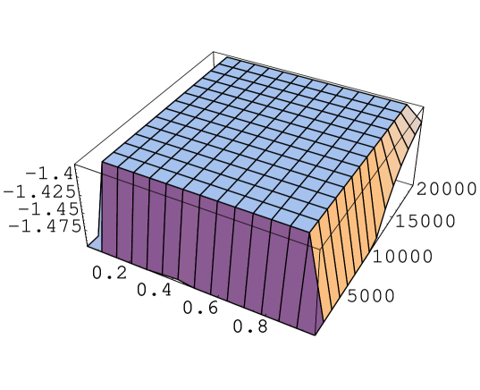
Figure 5: Behavior of $\ln|{\frac{1}{2}}{\cal F}^{-}({\tilde{k}},z)|=\ln|{\tilde{k}}\leavevmode\nobreak\ G^{-}_{k}(z,z)/(\omega z)^{3}|$. $\omega=10^{4},T=1,\Lambda=2\times 10^{4}$. $1.0001/\omega\leq z\leq 0.9999/T$. $\Lambda T/\omega\leq{\tilde{k}}\leq\Lambda$. Note $\ln|(1/2)\times(1/2)|\approx-1.39$.

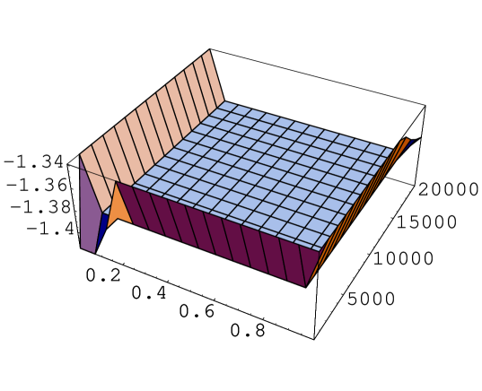
Figure 6: Behavior of $\ln|{\frac{1}{2}}{\cal F}^{+}({\tilde{k}},z)|=\ln|{\tilde{k}}\leavevmode\nobreak\ G^{+}_{k}(z,z)/(\omega z)^{3}|$. $\omega=10^{4},T=1,\Lambda=2\times 10^{4}$. $1.0001/\omega\leq z\leq 0.9999/T$. $\Lambda T/\omega\leq{\tilde{k}}\leq\Lambda$

4 UV and IR Regularization Parameters and Evaluation of Casimir Energy

The integral region of the above equation (45) is displayed in Fig.7. In the figure, we introduce the regularization cut-offs for the 4D-momentum integral, $\mu\leq{\tilde{p}}\leq\Lambda$. As for the extra-coordinate integral, it is the finite interval, $1/\omega\leq z\leq 1/T={\rm e}^{\omega l}/\omega$, hence we need not introduce further regularization parameters. For simplicity, we take the following IR cutoff of 4D momentum. :

$$\mu=\Lambda\cdot\frac{T}{\omega}=\Lambda{\rm e}^{-\omega l}{\quad.}$$ (48)

Hence the new regularization parameter is $\Lambda$ only.

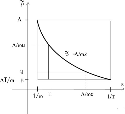
Figure 7: Space of (z,${\tilde{p}}$) for the integration. The hyperbolic curve will be used in Sec.5.

Let us evaluate the ($\Lambda,T$)-regularized value of (45).

$$-E_{Cas}^{\Lambda,\mp}(\omega,T)=\frac{2\pi^{2}}{(2\pi)^{4}}\int_{\mu}^{\Lambda}d{\tilde{p}}\int_{1/\omega}^{1/T}dz\leavevmode\nobreak\ {\tilde{p}}^{3}F^{\mp}({\tilde{p}},z){\quad,}$$

$$F^{\mp}({\tilde{p}},z)=\frac{2}{(\omega z)^{3}}\int_{\tilde{p}}^{\Lambda}{\tilde{k}}\leavevmode\nobreak\ G^{\mp}_{k}(z,z)d{\tilde{k}}{\quad.}$$ (49)

The integral region of (${\tilde{p}},z$) is the rectangle shown in Fig.7 .

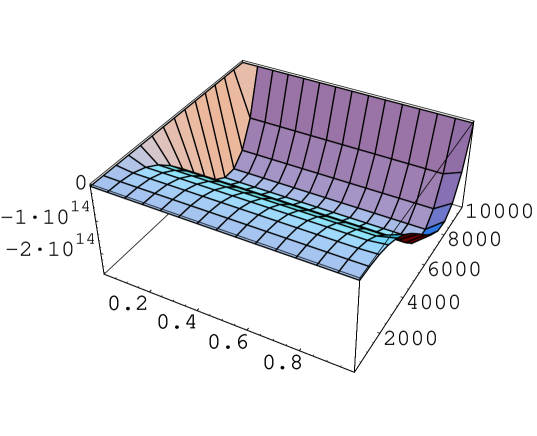
Figure 8: Behaviour of $(-1/2){\tilde{p}}^{3}F^{-}({\tilde{p}},z)$ (49). $T=1,\omega=10^{4},\Lambda=10^{4}$. $1.0001/\omega\leq z<0.9999/T$, $\Lambda T/\omega\leq{\tilde{p}}\leq\Lambda$ .

Figure 9: Behavior of $(-1/2){\tilde{p}}^{3}F^{-}({\tilde{p}},z)$ (49). $T=1,\omega=10^{4},\Lambda=2\cdot 10^{4}$. $1.0001/\omega\leq z<0.9999/T$, $\Lambda T/\omega\leq{\tilde{p}}\leq\Lambda$ .

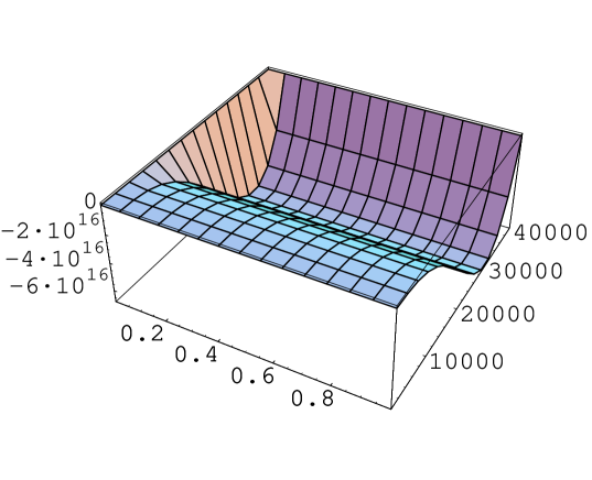
Figure 10: Behavior of $(-1/2){\tilde{p}}^{3}F^{-}({\tilde{p}},z)$ (49). $T=1,\omega=10^{4},\Lambda=4\cdot 10^{4}$. $1.0001/\omega\leq z<0.9999/T$, $\Lambda T/\omega\leq{\tilde{p}}\leq\Lambda$ .

Note that eq.(49) is the rigorous expression of the $(\Lambda,T)$-regularized Casimir energy. We show the behavior of $(-1/2){\tilde{p}}^{3}F^{-}({\tilde{p}},z)$ taking the values $\omega=10^{4},T=1$ in Fig.8($\Lambda=10^{4}$), Fig.9($\Lambda=2\cdot 10^{4}$) and Fig.10($\Lambda=4\cdot 10^{4}$). All three graphs have a common shape. (We confirm the graphs do not depend on the choice of $\omega$ and $T$ very much.) Behavior along ${\tilde{p}}$-axis does not so much depend on $z$. A valley runs parallel to the $z$-axis with the bottom line at the fixed ratio of ${\tilde{p}}/\Lambda\sim 0.75$. The depth of the valley is proportional to $\Lambda^{4}$. Because $E_{Cas}$ is the (${\tilde{p}},z$) ’flat-plane’ integral of ${\tilde{p}}^{3}F({\tilde{p}},z)$ , the volume inside the valley is the quantity $E_{Cas}$ . Hence it is easy to see $E_{Cas}$ is proportional to $\Lambda^{5}$. This is the same situation as the flat case (the upper eq. of (5)). Importantly, (49) shows the scaling behavior for large values of $\Lambda$ and $1/T$. From a close numerical analysis of (${\tilde{p}},z$)-integral (49) , we have confirmed

$$E^{\Lambda,-}_{Cas}(\omega,T)=\frac{2\pi^{2}}{(2\pi)^{4}}\times\left[-0.0250\frac{\Lambda^{5}}{T}\right]{\quad,}$$ (50)

which does not depend on $\omega$ and has no $\ln\frac{\Lambda}{T}$-term. (Note: $0.025=1/40$. See App.D for the numerical derivation.) Compared with the flat case (the upper eq. of (5)), we see the factor $T^{-1}$ plays the role of IR parameter of the extra space. We note that the behavior of Fig.8-10 is similar to the Rayleigh-Jeans’s region (small momentum region) of the Planck’s radiation formula (Fig.2) in the sense that ${\tilde{p}}^{3}F({\tilde{p}},z)\propto{\tilde{p}}^{3}$ for ${\tilde{p}}\ll\Lambda$.

Finally we notice, from the Fig.8-10, the approximate form of $F({\tilde{p}},z)$ for the large $\Lambda$ and $1/T$ is given by

$$F^{\mp}({\tilde{p}},z)\approx\frac{f}{2}\Lambda(1-\frac{{\tilde{p}}}{\Lambda}){\quad,}\quad f=1{\quad,}$$ (51)

which does not depend on $z,\omega$ and $T$. $f$ is the degree of freedom. The above result is consistent with (46).

5 UV and IR Regularization Surfaces, Principle of Minimal Area and Renormalization Flow

The advantage of the new approach is that the KK-expansion is replaced by the integral of the extra dimensional coordinate $z$ and all expressions are written in the closed ( not expanded ) form. The $\Lambda^{5}$-divergence, (50), shows the notorious problem of the higher dimensional theories, as in the flat case (the upper eq. of (5)). In spite of all efforts of the past literature, we have not succeeded in defining the higher-dimensional theories. (The divergence causes problems. The famous example is the divergent cosmological constant in the gravity-involving theories. [5] ) Here we notice that the divergence problem can be solved if we find a way to legitimately restrict the integral region in (${\tilde{p}},z$)-space.

One proposal of this was presented by Randall and Schwartz[29]. They introduced the position-dependent cut-off, $\mu<{\tilde{p}}<\Lambda/\omega u\ ,\ u\in[1/\omega,1/T]$ , for the 4D-momentum integral in the "brane" located at $z=u$. See Fig.7. The total integral region is the lower part of the hyperbolic curve ${\tilde{p}}=\Lambda/\omega z$. They succeeded in obtaining the finite $\beta$-function of the 5D warped vector model. We have confirmed that the value $E_{Cas}$ of (49), when the Randall-Schwartz integral region (Fig.7) is taken, is proportional to $\Lambda^{5}$. The close numerical analysis says

$$E^{-RS}_{Cas}(\omega,T)=\frac{2\pi^{2}}{(2\pi)^{4}}\int_{\mu}^{\Lambda}dq\int_{1/\omega}^{\Lambda/\omega q}dz\leavevmode\nobreak\ q^{3}F^{-}(q,z)=\frac{2\pi^{2}}{(2\pi)^{4}}\int_{1/\omega}^{1/T}du\int_{\mu}^{\Lambda/\omega u}d{\tilde{p}}\leavevmode\nobreak\ {\tilde{p}}^{3}F^{-}({\tilde{p}},u)$$

$$=\frac{2\pi^{2}}{(2\pi)^{4}}\frac{\Lambda^{5}}{\omega}\left\{-1.58\times 10^{-2}-1.69\times 10^{-4}\ln\leavevmode\nobreak\ \frac{\Lambda}{\omega}\right\}{\quad,}$$ (52)

which is independent of $T$ . This shows the divergence situation does not improve compared with the non-restricted case of (50). $T$ of (50) is replaced by the warp parameter $\omega$. This is contrasting with the flat case where $E^{RS}_{Cas}\propto-\Lambda^{4}$. (the lower eq. of (5)) The UV-behavior, however, does improve if we can choose the parameter $\Lambda$ in the way: $\Lambda\propto\omega$. This fact shows the parameter $\omega$ "smoothes" the UV-singularity to some extent.

Although they claim the holography is behind the procedure, the legitimateness of the restriction looks less obvious. We have proposed an alternate approach and given a legitimate explanation within the 5D QFT[31, 33, 26, 34]. Here we closely examine the new regularization.

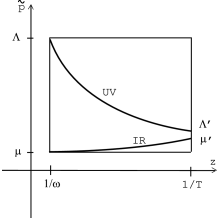
Figure 11: Space of (${\tilde{p}}$,z) for the integration (present proposal).

On the "3-brane" at $z=1/\omega$, we introduce the IR-cutoff $\mu=\Lambda\cdot\frac{T}{\omega}$ and the UV-cutoff $\Lambda$ ($\mu\ll\Lambda$). See Fig.11.

$$\mu\quad\ll\quad\Lambda\quad\quad(T\quad\ll\quad\omega){\quad.}$$ (53)

This is legitimate in the sense that we generally do this procedure in the 4D renormalizable thoeries. (Here we are considering those 5D theories that are renormalizable in "3-branes". Examples are 5D free theories (present model), 5D electromagnetism[26], 5D $\Phi^{4}$-theory, 5D Yang-Mills theory, e.t.c..) In the same reason, on the "3-brane" at $z=1/T$, we may have another set of IR and UV-cutoffs, $\mu^{\prime}$ and $\Lambda^{\prime}$. We consider the case:

$$\mu^{\prime}\leq\Lambda^{\prime},\ \Lambda^{\prime}\ll\Lambda,\ \mu\sim\mu^{\prime}{\quad.}$$ (54)

This case will lead us to introduce the renormalization flow. (See the later discussion.) We claim here, as for the regularization treatment of the "3-brane" located at other points $z$ ($1/\omega<z\leq 1/T$), the regularization parameters are determined by the minimal area principle. To explain it, we move to the 5D coordinate space ($x^{\mu},z$). See Fig.12.

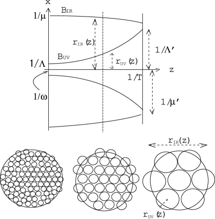
Figure 12: Regularization Surface $B_{IR}$ and $B_{UV}$ in the 5D coordinate space $(x^{\mu},z)$. The three graphs at the bottom show the flow of coarse graining (renormalization) and the sphere lattice regularization which will be explained after some paragraphs.

The ${\tilde{p}}$-expression can be replaced by $\sqrt{x_{\mu}x^{\mu}}$-expression by the reciprocal relation.

$$\sqrt{x_{\mu}(z)x^{\mu}(z)}\equiv r(z)\quad\leftrightarrow\quad\frac{1}{{\tilde{p}}(z)}{\quad.}$$ (55)

The UV and IR cutoffs change their values along $z$-axis and their trajectories make surfaces in the 5D bulk space $(x^{\mu},z)$. We require the two surfaces do not cross for the purpose of the renormalization group interpretation (discussed later). We call them UV and IR regularization (or boundary) surfaces($B_{UV},B_{IR}$).

$$\mbox{B}_{UV}\quad:\quad\sqrt{(x^{1})^{2}+(x^{2})^{2}+(x^{3})^{2}+(x^{4})^{2}}=r_{UV}(z){\quad,}\quad\frac{1}{\omega}<z<1/T{\quad,}$$

$$\mbox{B}_{IR}\quad:\quad\sqrt{(x^{1})^{2}+(x^{2})^{2}+(x^{3})^{2}+(x^{4})^{2}}=r_{IR}(z){\quad,}\quad\frac{1}{\omega}<z<1/T{\quad,}$$ (56)

where $r_{UV}(z)$ and $r_{IR}(z)$ are some functions of $z$ which are fixed by the minimal area principle. The cross sections of the regularization surfaces at $z$ are the spheres $S^{3}$ with the radii $r_{UV}(z)$ and $r_{IR}(z)$. Here we consider the Euclidean space for simplicity. The UV-surface is stereographically shown in Fig.13 and reminds us of the closed string propagation. Note that the boundary surface B_UV (and B_IR) is the 4 dimensional manifold.

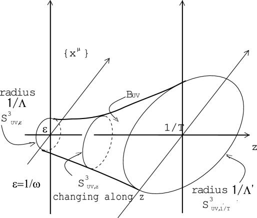
Figure 13: UV regularization surface ($B_{UV}$) in 5D coordinate space.

The 5D volume region bounded by $B_{UV}$ and $B_{IR}$ is the integral region of the Casimir energy $E_{Cas}$. The forms of $r_{UV}(z)$ and $r_{IR}(z)$ can be determined by the minimal area principle.

$$\delta(\mbox{Surface Area})=0{\quad,}$$

$$3+\frac{4}{z}r^{\prime}r-\frac{r^{\prime\prime}r}{{r^{\prime}}^{2}+1}=0{\quad,}\quad r^{\prime}\equiv\frac{dr}{dz}{\quad,}\quad r^{\prime\prime}\equiv\frac{d^{2}r}{dz^{2}}{\quad,}\quad 1/\omega\leq z\leq 1/T{\quad.}$$ (57)

In App.A, we present the classification of all solutions (paths). It helps to find appropriate minimal surface curves for the renormalization flow.

In Fig.14 we show two result curves of (57) taking the following boundary conditions ($r^{\prime}\equiv dr/dz$) :

Fig.11: Coarse Conf. goes to Fine Conf. as $$z$$ increases

$$\begin{array}[]{cc}\mbox{IR-curve (upper):}&r[1]=0.8,r^{\prime}[1]=1.0\quad\mbox{type\ (ia)}\\ \mbox{UV-curve (lower):}&r[1]=10^{-4},r^{\prime}[1]=-1.0\quad\mbox{type\ (ia)}\end{array}$$ (60)

Figure 14: Numerical Solution by Runge-Kutta. (57), Vertical axis: $r$; Horizontal axis: $z$. $T=1,\omega=10^{4},10^{-4}\leq z\leq 1.0$. Upper (B_IR): $r(1)=0.8,r^{\prime}(1)=1.0,$;   Lower (B_UV): $r(1)=10^{-4},r^{\prime}(1)=-1.0$ . Both curves are Graph Type (ia).

They show the flow of renormalization really occurs by the minimal area principle. (See the next paragraph for the renormalization flow interpretation.) These results imply the boundary conditions determine the property of the renormalization flow.

The present regularization scheme gives the renormalization group interpretation to the change of physical quantities along the extra axis. See Fig.12. In the "3-brane" located at $z$, the UV-cutoff is $r_{UV}(z)$ and the regularization surface is the sphere $S^{3}$ with the radius $r_{UV}(z)$. The IR-cutoff is $r_{IR}(z)$ and the regularization surface is the another sphere $S^{3}$ with the radius $r_{IR}(z)$. We can regard the regularization integral region as the sphere lattice of the following properties:

$$\mbox{A unit lattice (cell)\ :\ the sphere }S^{3}\mbox{\ with radius\ }r_{UV}(z)\mbox{and its inside}{\quad,}$$

$$\mbox{Total lattice\ :\ the sphere }S^{3}\mbox{with radius\ }r_{IR}(z)\ \mbox{and its inside}{\quad.}$$

$$\mbox{It is made of many cells above}{\quad,}$$

$$\mbox{Total number of cells\ :\ }\mbox{const.}\times\left(\frac{r_{IR}(z)}{r_{UV}(z)}\right)^{4}{\quad.}$$ (61)

The total number of cells changes from $(\frac{\Lambda}{\mu})^{4}$ at $z=1/\omega$ to $(\frac{\Lambda^{\prime}}{\mu^{\prime}})^{4}$ at $z=1/T$. Along the $z$-axis, the number increases or decreases as

$$\left(\frac{r_{IR}(z)}{r_{UV}(z)}\right)^{4}\equiv N(z){\quad.}$$ (62)

For the "scale" change $z\rightarrow z+\Delta z$, $N$ changes as

$$\Delta(\ln N)=4\frac{\partial}{\partial z}\{\ln(\frac{r_{IR}(z)}{r_{UV}(z)})\}\cdot\Delta z{\quad.}$$ (63)

When the system has some coupling $g(z)$, the renormalization group ${\tilde{\beta}}(g)$-function (along the extra axis) is expressed as

$${\tilde{\beta}}=\frac{\Delta(\ln g)}{\Delta(\ln N)}=\frac{1}{\Delta(\ln N)}\frac{\Delta g}{g}=\frac{1}{4}\frac{1}{\frac{\partial}{\partial z}\ln(\frac{r_{IR}(z)}{r_{UV}(z)})}\frac{1}{g}\frac{\partial g}{\partial z}{\quad,}$$ (64)

where $g(z)$ is a renormalized coupling at $z$.

We have explained, in this section, that the minimal area principle determines the flow of the regularization surfaces.

6 Weight Function and Casimir Energy Evaluation

In the expression (43), the Casimir energy is written by the integral in the (${\tilde{p}},z$)-space over the range: $1/\omega\leq z\leq 1/T,\ 0\leq{\tilde{p}}\leq\infty$. In Sec.5, we have seen the integral region should be properly restricted because the cut-off region in the 4D world changes along the extra-axis obeying the bulk (warped) geometry (minimal area principle). We can expect the singular behavior (UV divergences) reduces by the integral-region restriction, but the concrete evaluation along the proposed prescription is practically not easy. In this section, we consider an alternate approach which respects the minimal area principle and evaluate the Casimir energy.

We introduce, instead of restricting the integral region, a weight function $W({\tilde{p}},z)$ in the (${\tilde{p}},z$)-space for the purpose of suppressing UV and IR divergences of the Casimir Energy.

$$-E^{\mp\leavevmode\nobreak\ W}_{Cas}(\omega,T)\equiv{\int\frac{d^{4}p_{E}}{(2\pi)^{4}}}\int_{1/\omega}^{1/T}dz\leavevmode\nobreak\ W({\tilde{p}},z)F^{\mp}({\tilde{p}},z){\quad,}\quad{\tilde{p}}=\sqrt{p_{4}^{2}+p_{1}^{2}+p_{2}^{2}+p_{3}^{2}}{\quad,}$$

$$F^{\mp}({\tilde{p}},z)=s(z)\int_{p^{2}}^{\infty}\{G_{k}^{\mp}(z,z)\}dk^{2}=\frac{2}{(\omega z)^{3}}\int_{\tilde{p}}^{\infty}{\tilde{k}}\leavevmode\nobreak\ G^{\mp}_{k}(z,z)d{\tilde{k}}{\quad,}$$

$$\mbox{Examples of}\leavevmode\nobreak\ W({\tilde{p}},z):\quad W({\tilde{p}},z)=\hskip 284.52756pt$$

$$\left\{\begin{array}[]{cc}(N_{1})^{-1}{\rm e}^{-(1/2){\tilde{p}}^{2}/\omega^{2}-(1/2)z^{2}T^{2}}\equiv W_{1}({\tilde{p}},z),\ N_{1}=1.711/8\pi^{2}&\mbox{elliptic suppr.}\\ (N_{1b})^{-1}{\rm e}^{-(1/2){\tilde{p}}^{2}/\omega^{2}}\equiv W_{1b}({\tilde{p}},z),\ N_{1b}=2/8\pi^{2}&\mbox{kinetic-energy suppr.}\\ (N_{2})^{-1}{\rm e}^{-{\tilde{p}}zT/\omega}\equiv W_{2}({\tilde{p}},z),\ N_{2}=2\frac{\omega^{3}}{T^{3}}/8\pi^{2}&\mbox{hyperbolic suppr.1}\\ (N_{3})^{-1}{\rm e}^{-(1/2){\tilde{p}}^{2}z^{2}T^{2}/\omega^{2}}\equiv W_{3}({\tilde{p}},z),\ N_{3}=\frac{2}{3}\frac{\omega^{3}}{T^{3}}/8\pi^{2}&\mbox{hyperbolic suppr.2}\\ (N_{4})^{-1}{\rm e}^{-(1/2){\tilde{p}}^{2}/z^{2}\omega^{2}T^{2}}\equiv W_{4}({\tilde{p}},z),\ N_{4}=\frac{2}{5}/8\pi^{2}&\mbox{linear suppr.}\\ (N_{5})^{-1}{\rm e}^{-{\tilde{p}}/z^{2}\omega T^{2}}\equiv W_{5}({\tilde{p}},z),\ N_{5}=\frac{2}{3}/8\pi^{2}&\mbox{parabolic suppr.1}\\ (N_{6})^{-1}{\rm e}^{-{\tilde{p}}^{2}/2z\omega^{2}T}\equiv W_{6}({\tilde{p}},z),\ N_{6}=\frac{2}{3}/8\pi^{2}&\mbox{parabolic suppr.2}\\ (N_{7})^{-1}{\rm e}^{-(1/2){\tilde{p}}^{4}/\omega^{4}}\equiv W_{7}({\tilde{p}},z),\ N_{7}=\frac{1}{2}/8\pi^{2}&\mbox{higher-der. suppr.1}\\ (N_{8})^{-1}{\rm e}^{-1/2({\tilde{p}}^{2}/\omega^{2}+1/z^{2}T^{2})}\equiv W_{8}({\tilde{p}},z),\ N_{8}=0.4177/8\pi^{2}&\mbox{reciprocal suppr.1}\\ (N_{47})^{-1}{\rm e}^{-1/2({\tilde{p}}^{2}/\omega^{2})({\tilde{p}}^{2}/\omega^{2}+1/z^{2}T^{2})}\equiv W_{47}({\tilde{p}},z),\ N_{47}=0.1028/8\pi^{2}&\mbox{higher-der. suppr.2}\\ (N_{56})^{-1}{\rm e}^{-1/2({\tilde{p}}/z\omega T)({\tilde{p}}/\omega+1/zT)}\equiv W_{56}({\tilde{p}},z),\ N_{56}=0.1779/8\pi^{2}&\mbox{reciprocal suppr.2}\\ (N_{88})^{-1}{\rm e}^{-1/2({\tilde{p}}^{2}/\omega^{2}+1/z^{2}T^{2})^{2}}\equiv W_{88}({\tilde{p}},z),\ N_{88}=0.01567/8\pi^{2}&\mbox{higher-der. reciprocal suppr.}\\ (N_{9})^{-1}{\rm e}^{-1/2({\tilde{p}}/\omega+1/zT)^{2}}\equiv W_{9}({\tilde{p}},z),\ N_{9}=0.05320/8\pi^{2}&\mbox{reciprocal suppr.3}\\ \end{array}\right.$$ (78)

where $G_{k}^{\mp}(z,z)$ are defined in (44). The normalization constants $N_{i}$ are explained in App.E. In the above, we list some examples expected for the weight function $W({\tilde{p}},z)$. $W_{2}$ and $W_{3}$ are regarded to correspond to the regularization taken by Randall-Schwartz. How to specify the form of $W$ is the subject of the next section. We show the shape of the energy integrand $(-1/2){\tilde{p}}^{3}W({\tilde{p}},z)F^{-}({\tilde{p}},z)$ in Fig.15-18 for various choices of $W$. We notice the valley-bottom line ${\tilde{p}}\approx 0.75\Lambda$, which appeared in the un-weighted case (Fig.8-10), is replaced by new lines: ${\tilde{p}}^{2}+z^{2}\times\omega^{2}T^{2}\approx\mbox{const}$(Fig.15,$W_{1}$), ${\tilde{p}}z\approx\mbox{const}$ (Fig.16,$W_{3}$), ${\tilde{p}}\approx\mbox{const}\times z$(Fig.17,$W_{4}$), ${\tilde{p}}\approx\mbox{const}\times\sqrt{z}$ (Fig.18,$W_{6}$). They are all located away from the original $\Lambda$-effected line (${\tilde{p}}\sim 0.75\Lambda$).

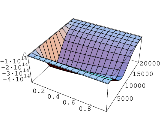
Figure 15: Behavior of $(-N_{1}/2){\tilde{p}}^{3}W_{1}({\tilde{p}},z)F^{-}({\tilde{p}},z)$(elliptic suppression). $\Lambda=20000,\ \omega=5000,\ T=1$ . $1.0001/\omega\leq z\leq 0.9999/T,\ \mu=\Lambda T/\omega\leq{\tilde{p}}\leq\Lambda$.

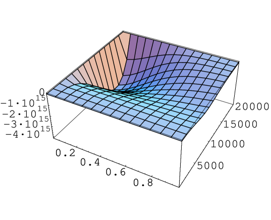
Figure 16: Behavior of $(-N_{3}/2){\tilde{p}}^{3}W_{3}({\tilde{p}},z)F^{-}({\tilde{p}},z)$(hyperbolic suppression2). $\Lambda=20000,\ \omega=5000,\ T=1$ . $1.0001/\omega\leq z\leq 0.9999/T,\ \mu=\Lambda T/\omega\leq{\tilde{p}}\leq\Lambda$.

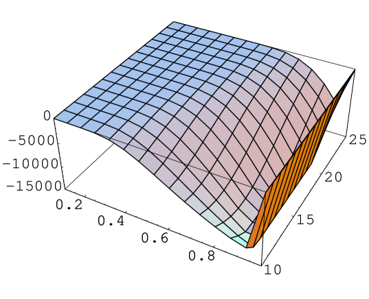
Figure 17: Behavior of $(-N_{4}/2){\tilde{p}}^{3}W_{4}({\tilde{p}},z)F^{-}({\tilde{p}},z)$(linear suppression). $\Lambda=100,\ \omega=10,\ T=1$ . $1.0001/\omega\leq z\leq 0.9999/T,\ \mu=\Lambda T/\omega\leq{\tilde{p}}\leq 25$. In order to demonstrate the valley-bottom line is similar to a minimal surface line (See App.C), we here take rather small values of $\Lambda$ and $\omega$. The contour of this graph will be shown later.

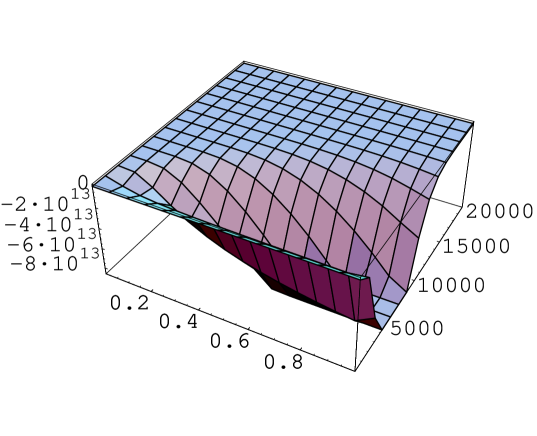
Figure 18: Behavior of $(-N_{6}/2){\tilde{p}}^{3}W_{6}({\tilde{p}},z)F^{-}({\tilde{p}},z)$(parabolic suppression2). $\Lambda=20000,\ \omega=5000,\ T=1$ . $1.0001/\omega\leq z\leq 0.9999/T,\ \mu=\Lambda T/\omega\leq{\tilde{p}}\leq\Lambda$.

We can check the divergence (scaling) behavior of $E^{\mp\leavevmode\nobreak\ W}_{Cas}$ by numerically evaluating the $({\tilde{p}},z)$-integral (78) for the rectangle region of Fig.7.

$$-E^{W}_{Cas}=\mbox{\hskip 284.52756pt}$$

$$\left\{\begin{array}[]{cc}\frac{\omega^{4}}{T}\Lambda\times 1.2\left\{1+0.11\leavevmode\nobreak\ \ln\frac{\Lambda}{\omega}-0.10\leavevmode\nobreak\ \ln\frac{\Lambda}{T}\right\}&\mbox{for}\quad W_{1}\\ \frac{\omega^{4}}{T}\Lambda\times 2.0\left\{1+0.07\leavevmode\nobreak\ \ln\frac{\Lambda}{\omega}-0.10\leavevmode\nobreak\ \ln\frac{\Lambda}{T}\right\}&\mbox{for}\quad W_{1b}\\ \frac{T^{2}}{\omega^{2}}\Lambda^{4}\times 0.062\left\{1+0.03\leavevmode\nobreak\ \ln\frac{\Lambda}{\omega}-0.08\leavevmode\nobreak\ \ln\frac{\Lambda}{T}\right\}&\mbox{for}\quad W_{2}\\ \frac{T^{2}}{\omega^{2}}\Lambda^{4}\times 0.14\left\{1+0.01\leavevmode\nobreak\ \ln\frac{\Lambda}{\omega}-0.06\leavevmode\nobreak\ \ln\frac{\Lambda}{T}\right\}&\mbox{for}\quad W_{3}\\ \frac{\omega^{4}}{T}\Lambda\times 1.5\left\{1+0.08\leavevmode\nobreak\ \ln\frac{\Lambda}{\omega}-0.10\leavevmode\nobreak\ \ln\frac{\Lambda}{T}\right\}&\mbox{for}\quad W_{4}\\ \frac{\omega^{4}}{T}\Lambda\times 1.5\left\{1+0.07\leavevmode\nobreak\ \ln\frac{\Lambda}{\omega}-0.10\leavevmode\nobreak\ \ln\frac{\Lambda}{T}\right\}&\mbox{for}\quad W_{5}\\ \frac{\omega^{4}}{T}\Lambda\times 0.86\left\{1+0.07\leavevmode\nobreak\ \ln\frac{\Lambda}{\omega}-0.07\leavevmode\nobreak\ \ln\frac{\Lambda}{T}\right\}&\mbox{for}\quad W_{6}\\ \frac{\omega^{4}}{T}\Lambda\times 1.3\left\{1+0.06\leavevmode\nobreak\ \ln\frac{\Lambda}{\omega}-0.08\leavevmode\nobreak\ \ln\frac{\Lambda}{T}\right\}&\mbox{for}\quad W_{7}\\ \frac{\omega^{4}}{T}\Lambda\times 1.6\left\{1+0.09\leavevmode\nobreak\ \ln\frac{\Lambda}{\omega}-0.10\leavevmode\nobreak\ \ln\frac{\Lambda}{T}\right\}&\mbox{for}\quad W_{8}\\ \frac{\omega^{4}}{T}\Lambda\times 0.47\left\{1+0.05\leavevmode\nobreak\ \ln\frac{\Lambda}{\omega}-0.07\leavevmode\nobreak\ \ln\frac{\Lambda}{T}\right\}&\mbox{for}\quad W_{47}\\ \frac{\omega^{4}}{T}\Lambda\times 0.93\left\{1+0.06\leavevmode\nobreak\ \ln\frac{\Lambda}{\omega}-0.07\leavevmode\nobreak\ \ln\frac{\Lambda}{T}\right\}&\mbox{for}\quad W_{56}\\ \frac{\omega^{4}}{T}\Lambda\times 1.1\left\{1+0.06\leavevmode\nobreak\ \ln\frac{\Lambda}{\omega}-0.07\leavevmode\nobreak\ \ln\frac{\Lambda}{T}\right\}&\mbox{for}\quad W_{88}\\ \frac{\omega^{4}}{T}\Lambda\times 0.91\left\{1+0.05\leavevmode\nobreak\ \ln\frac{\Lambda}{\omega}-0.07\leavevmode\nobreak\ \ln\frac{\Lambda}{T}\right\}&\mbox{for}\quad W_{9}\end{array}\right.$$ (92)

The suppression behaviors of $W_{2}$ and $W_{3}$ improve, compared with (52) by Randall-Schwartz. The quintic divergence of (52) reduces to the quartic divergence in the present approach of $W_{2}$ and $W_{3}$. The hyperbolic suppressions, however, are still insufficient for the renormalizability. After dividing by the normalization factor, $\Lambda T^{-1}$, the cubic divergence remains. The desired cases are others. The Casimir energy for each case consists of three terms. The first terms give finite values after dividing by the overall normalization factor $\Lambda T^{-1}$. The last two terms are proportional to $\log\Lambda$ and show the anomalous scaling. Their contributions are order of $10^{-1}$ to the first leading terms. The second ones ($\ln\frac{\Lambda}{\omega}$) contribute positively while the third ones ($\ln\frac{\Lambda}{T}$) negatively.

They give, after normalizing the factor $\Lambda/T$, only the log-divergence.

$$E^{W}_{Cas}/\Lambda T^{-1}=-\alpha\omega^{4}\left(1-4c\ln(\Lambda/\omega)-4c^{\prime}\ln(\Lambda/T)\right){\quad,}$$ (93)

where $\alpha,c$ and $c^{\prime}$ can be read from (92) depending on the choice of $W$. This means the 5D Casimir energy is finitely obtained by the ordinary renormalization of the warp factor $\omega$. (See the final section.) In the above result of the warped case, the IR parameter $l$ in the flat result (10) is replaced by the inverse of the warp factor $\omega$.

At present, we cannot discriminate which weight is the right one. Here we list characteristic features (advantageous(Yes) or disadvantageous(No), independent (I) or dependent(D), singular(S) or regular(R)) for each weight from the following points.

point 1

The behavior of $W$ for the limits: $T\rightarrow\infty$ (4D limit) ; $T\rightarrow 0$ (5D limit) ; $\omega\rightarrow 0$ (flat limit). This property is related to the continuation to the ordinary field-quantization.

point 2

How the path (bottom line of the valley) depends on the scales $T$ and $\omega$.

point 3

Regular(R) or singular(S) at $z=0$. This point is not important because the range of $z$ is $1/\omega\leq z\leq 1/T$ or $-1/T\leq z\leq-1/\omega$.

point 4

Symmetric for ${\tilde{p}}/\omega\leftrightarrow Tz$.

point 5

Symmetric for ${\tilde{p}}/\omega\leftrightarrow 1/Tz$. (Reciprocal symmetry)

point 6

The value of $\alpha$.

point 7

The values of (-4$c$,-4$c^{\prime}$).

point 8

Under the Z₂-parity $z\leftrightarrow-z$, $W({\tilde{p}},z)$ is even (E), odd (O) or none (N).

$$\begin{array}[]{|c|c|c|c|c|c|c|c|c|}\mbox{W type}&W_{1}&W_{1b}&W_{2}&W_{3}&W_{4}&W_{5}&W_{6}&W_{7}\\ \hline\cr\mbox{point 1}&&&&&&&&\\ \mbox{$T\rightarrow\infty$}&T^{-1}\times&/&(\frac{\omega}{T})^{-3+1/2}\times&(\frac{\omega}{T})^{-3+1}\times&/&/&/&/\\ &\delta(z)&/&\delta(\sqrt{{\tilde{p}}z})&\delta({\tilde{p}}z)&/&/&/&/\\ \mbox{$T\rightarrow 0$}&/&/&/&/&T\omega\times&T\sqrt{\omega}\times&\sqrt{T}\omega\times&/\\ &/&/&/&/&\delta({\tilde{p}}/z)&\delta(\sqrt{{\tilde{p}}}/z)&\delta({\tilde{p}}/\sqrt{z})&/\\ \mbox{$\omega\rightarrow 0$}&\omega\times&\omega\times&(\frac{\omega}{T})^{-3+1/2}\times&(\frac{\omega}{T})^{-3+1}\times&T\omega\times&T\sqrt{\omega}\times&\sqrt{T}\omega\times&\omega^{2}\times\\ &\delta({\tilde{p}})&\delta({\tilde{p}})&\delta(\sqrt{{\tilde{p}}z})&\delta({\tilde{p}}z)&\delta(\frac{{\tilde{p}}}{z})&\delta(\sqrt{{\tilde{p}}}/z)&\delta({\tilde{p}}/\sqrt{z})&\delta({\tilde{p}}^{2})\\ \mbox{point 2}&\omega,T&\omega&T/\omega&T/\omega&\omega T&\omega T^{2}&\omega^{2}T&\omega\\ \mbox{point 3}&(R)&(R)&(R)&(R)&(S)&(S)&(S)&(R)\\ \mbox{point 4}&Y&/&Y&Y&/&N&N&/\\ \mbox{point 5}&/&/&/&/&Y&N&N&/\\ \mbox{point 6}&1.2&2.0&div.&div.&1.5&1.5&0.86&1.3\\ \mbox{point 7}&&&&&&&&\\ -4c&0.11&0.07&0.03&0.01&0.08&0.07&0.07&0.06\\ -4c^{\prime}&-0.10&-0.10&-0.08&-0.06&-0.10&-0.10&-0.07&-0.08\\ \mbox{point 8}&E&E&O&E&E&E&O&E\end{array}$$

$$\begin{array}[]{|c|c|c|c|c|c|}\mbox{W type}&W_{8}&W_{47}&W_{56}&W_{88}&W_{9}\\ \hline\cr\mbox{point 1}&&&&&\\ \mbox{$T\rightarrow\infty$}&/&/&/&/&/\\ &/&/&/&/&/\\ \mbox{$T\rightarrow 0$}&T\times&T\omega\times&T\sqrt{\omega}\times&T^{2}\times&T\times\\ &\delta(\frac{1}{z})&\delta(\frac{{\tilde{p}}}{z})&\delta(\sqrt{{\tilde{p}}}/z)&\delta(\frac{1}{z^{2}})&\delta(\frac{1}{z})\\ \mbox{$\omega\rightarrow 0$}&\omega\times&\omega^{2}\times&\omega\sqrt{T}\times&\omega^{2}\times&\omega\times\\ &\delta({\tilde{p}})&\delta({\tilde{p}}^{2})&\delta({\tilde{p}}/\sqrt{z})&\delta({\tilde{p}}^{2})&\delta({\tilde{p}})\\ \mbox{point 2}&\omega,T&\omega,T&\omega,T&\omega,T&\omega,T\\ \mbox{point 3}&(S)&(S)&(S)&(S)&(S)\\ \mbox{point 4}&/&N&/&/&/\\ \mbox{point 5}&Y&N&Y&Y&Y\\ \mbox{point 6}&1.6&0.47&0.93&1.1&0.91\\ \mbox{point 7}&&&&&\\ -4c&0.09&0.05&0.06&0.06&0.05\\ -4c^{\prime}&-0.10&-0.07&-0.07&-0.07&-0.07\\ \mbox{point 8}&E&E&N&E&N\end{array}$$

We notice $W_{1}$ and $W_{8}$ are specially important.

So far as the legitimate reason of the introduction of $W({\tilde{p}},y)$ is not clear, we should regard this procedure as a regularization to define the higher dimensional theories. We give a clear definition of $W({\tilde{p}},y)$ and a legitimate explanation in the next section. It should be done, in principle, in a consistent way with the bulk geometry and the gauge principle.

7 Meaning of Weight Function and Quantum Fluctuation of Coordinates and Momenta

In the previous work[26], we have presented the following idea to define the weight function $W({\tilde{p}},z)$. In the evaluation (78):

$$-E^{W}_{Cas}(\omega,T)={\int\frac{d^{4}p_{E}}{(2\pi)^{4}}}\int_{1/\omega}^{1/T}dz\leavevmode\nobreak\ W({\tilde{p}},z)F^{\mp}({\tilde{p}},z)$$

$$=\frac{2\pi^{2}}{(2\pi)^{4}}\int d{\tilde{p}}\int_{1/\omega}^{1/T}dz\leavevmode\nobreak\ {\tilde{p}}^{3}W({\tilde{p}},z)F^{\mp}({\tilde{p}},z){\quad,}$$ (94)

the $({\tilde{p}},z)$-integral is over the rectangle region shown in Fig.11 (with $\Lambda\rightarrow\infty$ and $\mu\rightarrow 0$). $F^{\mp}({\tilde{p}},z)$ is explicitly given in (45). Following Feynman[35], we can replace the integral by the summation over all possible pathes ${\tilde{p}}(z)$ as schematically shown in Fig.19.

Figure 19: The mesh of the dotted lines shows the the ordinary integral of $\int d{\tilde{p}}dz$. Two solid lines show two pathes ${\tilde{p}}_{1}(z)$ and ${\tilde{p}}_{2}(z)$. The path-integral $\int{\cal D}{\tilde{p}}(z)$ is the integral over all possible pathes.

$$-E^{W}_{Cas}(\omega,T)=\int{\cal D}{\tilde{p}}(z)\int_{1/\omega}^{1/T}dz\leavevmode\nobreak\ S[{\tilde{p}}(z),z]{\quad,}$$

$$S[{\tilde{p}}(z),z]=\frac{2\pi^{2}}{(2\pi)^{4}}{\tilde{p}}(z)^{3}W({\tilde{p}}(z),z)F^{\mp}({\tilde{p}}(z),z){\quad.}$$ (95)

Especially, in the figure, the mesh shows the independency of the integral-variables $p^{a}$ and $z$. Two pathes ${\tilde{p}}_{1}(z)$ and ${\tilde{p}}_{2}(z)$ are shown as two solid lines. There exists the dominant path ${\tilde{p}}_{W}(z)$ which is determined by the minimal principle : $\delta S=0$.

$$\mbox{Dominant Path }{\tilde{p}}_{W}(z)\ :\ \quad\frac{d{\tilde{p}}}{dz}=\frac{-\frac{\partial\ln(WF)}{\partial z}}{\frac{3}{{\tilde{p}}}+\frac{\partial\ln(WF)}{\partial{\tilde{p}}}}{\quad.}$$ (96)

Hence it is fixed by $W({\tilde{p}},z)$. Examples are the valley-bottom lines in Fig.15-18. On the other hand, there exists another independent path: the minimal surface curve $r_{g}(z)$.

$$\mbox{Minimal Surface Curve }r_{g}(z)\ :\quad 3+\frac{4}{z}r^{\prime}r-\frac{r^{\prime\prime}r}{{r^{\prime}}^{2}+1}=0{\quad,}\quad\frac{1}{\omega}\leq z\leq\frac{1}{T}{\quad,}$$ (97)

which is obtained by the minimal area principle:

$$ds^{2}=\frac{1}{\omega^{2}z^{2}}(\delta_{ab}+\frac{x^{a}x^{b}}{(rr^{\prime})^{2}})dx^{a}dx^{b}\equiv g_{ab}(x)dx^{a}dx^{b}{\quad,}$$

$$\delta A=0{\quad,}\quad A=\int\sqrt{\det g_{ab}}\leavevmode\nobreak\ d^{4}x=\int_{1/\omega}^{1/T}\frac{1}{\omega^{4}z^{4}}\sqrt{{r^{\prime}}^{2}+1}\leavevmode\nobreak\ r^{3}dz{\quad.}$$ (98)

See App.A for detail. Hence $r_{g}(z)$ is fixed by the induced geometry $g_{ab}(x)$. Here we put the requirement[26]:

$${\tilde{p}}_{W}(z)={\tilde{p}}_{g}(z){\quad,}$$ (99)

where ${\tilde{p}}_{g}\equiv 1/r_{g}$. This means the following things. We require the dominant path coincides with the minimal surface line ${\tilde{p}}_{g}(z)=1/r_{g}(z)$ which is defined independently of $W({\tilde{p}},z)$. In other words, $W({\tilde{p}},z)$ is defined here by the induced geometry $g_{ab}(x)$. In this way, we can connect the integral-measure over the 5D-space with the (bulk) geometry. We have confirmed the (approximate) coincidence by the numerical method.(See App.C)

In order to most naturally accomplish the above requirement, we can go to a new step. Namely, we propose to replace the 5D space integral with the weight $W$, (94), by the following path-integral. We newly define the Casimir energy in the higher-dimensional theory as follows.

$$-{\cal E}_{Cas}(\omega,T,\Lambda)\equiv\int_{1/\Lambda}^{1/\mu}d\rho\int_{{\tilde{p}}(1/\omega)={\tilde{p}}(1/T)=1/\rho}\prod_{a,z}{\cal D}p^{a}(z)F({\tilde{p}},z)$$

$$\times\exp\left[-\frac{1}{2\alpha^{\prime}}\int_{1/\omega}^{1/T}\frac{1}{\omega^{4}z^{4}}\frac{1}{{\tilde{p}}^{3}}\sqrt{\frac{{\tilde{p}}^{{}^{\prime}2}}{{\tilde{p}}^{4}}+1}\leavevmode\nobreak\ dz\right]$$

$$=\int_{1/\Lambda}^{1/\mu}d\rho\int_{r(1/\omega)=r(1/T)=\rho}\prod_{a,z}{\cal D}x^{a}(z)F(\frac{1}{r},z)$$

$$\times\exp\left[-\frac{1}{2\alpha^{\prime}}\int_{1/\omega}^{1/T}\frac{1}{\omega^{4}z^{4}}\sqrt{{r^{\prime}}^{2}+1}\leavevmode\nobreak\ r^{3}dz\right]{\quad,}$$ (100)

where $\mu=\Lambda T/\omega$ and the limit $\Lambda T^{-1}\rightarrow\infty$ is taken. The string (surface) tension parameter $1/2\alpha^{\prime}$ is introduced. (Note: Dimension of $\alpha^{\prime}$ is [Length]⁴. ) The square-bracket ($[\cdots]$)-parts of (100) are  $-\frac{1}{2\alpha^{\prime}}$Area = $-\frac{1}{2\alpha^{\prime}}\int\sqrt{\mbox{det}g_{ab}}d^{4}x$ (See (114)) where $g_{ab}$ is the induced metric on the 4D surface. $F({\tilde{p}},z)$ is defined in (78) or (45) and shows the field-quantization of the bulk scalar (EM) fields. In the above expression, we have followed the path-integral formulation of the density matrix (See Feynman’s text[35]). The validity of the above definition is based on the following points: a) When the weight part (exp $[\cdots]$-part) is 1, the proposed quantity ${\cal E}_{Cas}$ is equal to $E^{W}_{Cas}$, (94), with $W=1$ ; b) The leading path is given by $r_{g}(z)=1/p_{g}(z)$, (97); c) The proposed definition, (100), clearly shows the 4D space-coordinates $x^{a}$ or the 4D momentum-coordinates $p^{a}$ are quantized (quantum-statistically, not field-theoretically) with the Euclidean time $z$ and the "area Hamiltonian" $A=\int\sqrt{\det g_{ab}}\leavevmode\nobreak\ d^{4}x$. Note that $F({\tilde{p}},z)$ or $F(1/r,z)$ appears, in (100), as the energy density operator in the quantum statistical system of $\{p^{a}(z)\}$ or $\{x^{a}(z)\}$.

In the view of the previous paragraph, the treatment of Sec.6 is an effective action approach using the (trial) weight function $W({\tilde{p}},z)$. Note that the integral over $(p^{\mu},z)$-space, appearing in (45), is the summation over all degrees of freedom of the 5D space(-time) points using the "naive" measure $d^{4}pdz$. An important point is that we have the possibility to take another measure for the summation in the case of the higher dimensional QFT. We have adopted, in Sec.6, the new measure $W(p^{\mu},z)d^{4}pdz$ in such a way that the Casimir energy does not show physical divergences. We expect the direct evaluation of (100), numerically or analytically, leads to the similar result.

8 Discussion and Conclusion

The log-divergence in (93) is the familiar one in the ordinary QFT. It can be renormalized in the following way.

$$E^{W}_{Cas}/\Lambda T^{-1}=-\alpha\omega^{4}\left(1-4c\ln(\Lambda/\omega)-4c^{\prime}\ln(\Lambda/T)\right)=-\alpha(\omega_{r})^{4}{\quad,}$$

$$\omega_{r}=\omega\sqrt[4]{1-4c\ln(\Lambda/\omega)-4c^{\prime}\ln(\Lambda/T)}{\quad,}$$ (101)

where $\omega_{r}$ is the renormalized warp factor and $\omega$ is the bare one. No local counterterms are necessary. Note that this renormalization relation is exact (not a perturbative result). In the familiar case of the 4D renormalizable theories, the coefficients $c$ and $c^{\prime}$ depend on the coupling, but, in the present case, they are pure numbers. It reflects the interaction between (EM) fields and the boundaries. When $c$ and $c^{\prime}$ are sufficiently small we find the renormalization group function for the warp factor $\omega$ as

$$|c|\ll 1{\quad,}\quad|c^{\prime}|\ll 1{\quad,}\quad\omega_{r}=\omega(1-c\ln(\Lambda/\omega)-c^{\prime}\ln(\Lambda/T)){\quad,}$$

$$\beta(\mbox{$\beta$-function})\equiv\frac{\partial}{\partial(\ln\Lambda)}\ln\frac{\omega_{r}}{\omega}=-c-c^{\prime}{\quad.}$$ (102)

We should notice that, in the flat geometry case, the IR parameter (extra-space size) $l$ is renormalized (see Sec.1). In the present warped case, however, the corresponding parameter $T$ is not renormalized, but the warp parameter $\omega$ is renormalized. Depending on the sign of $c+c^{\prime}$, the 5D bulk curvature $\omega$ flows as follows. When $c+c^{\prime}>0$, the bulk curvature $\omega$ decreases (increases) as the the measurement energy scale $\Lambda$ increases (decreases). When $c+c^{\prime}<0$, the flow goes in the opposite way. When $c+c^{\prime}=0$, $\omega$ does not flow ($\beta=0$) and is given by $\omega_{r}=\omega(1+c\ln(\omega/T))$.

The final result (101) is the new type Casimir energy, $-\omega^{4}$. $\omega$ appears as a boundary parameter like $T$. The familiar one is $-T^{4}$ in the present context (See (10). Note $T$ is the IR parameter and is related to $l$ as $T=\omega{\rm e}^{-\omega l}$.). In ref.[36], another type $T^{2}\omega^{2}$ was predicted using a "quasi" Warped model (bulk-boundary theory).

Through the Casimir energy calculation, in the higher dimension, we find a way to quantize the higher dimensional theories within the QFT framework. The quantization with respect to the fields (except the gravitational fields $G_{AB}(X)$) is done in the standard way. After this step, the expression has the summation over the 5D space(-time) coordinates or momenta $\int dz\prod_{a}dp^{a}$. We have proposed that this summation should be replaced by the path-integral $\int\prod_{a,z}{\cal D}p^{a}(z)$ with the area action (Hamiltonian) $A=\int\sqrt{\det g_{ab}}d^{4}x$ where $g_{ab}$ is the induced metric on the 4D surface. This procedure says the 4D momenta $p^{a}$ (or coordinates $x^{a}$) are quantum statistical operators and the extra-coordinate $z$ is the inverse temperature (Euclidean time). We recall the similar situation occurs in the standard string approach. The space-time coordinates obey some uncertainty principle[37].

Recently the dark energy ( as well as the dark matter ) in the universe is a hot subject. It is well-known that the dominant candidate is the cosmological term. We also know the proto-type higher-dimensional theory, that is, the 5D KK theory, has predicted so far the divergent cosmological constant[5]. This unpleasant situation has been annoying us for a long time. If we apply the present result, the situation drastically improve. The cosmological constant $\lambda$ appears as

$$R_{\mu\nu}-{\frac{1}{2}}g_{\mu\nu}R-\lambda g_{\mu\nu}=T_{\mu\nu}^{matter}{\quad,}$$

$$S=\int d^{4}x\sqrt{-g}\{\frac{1}{G_{N}}(R+\lambda)\}+\int d^{4}x\sqrt{-g}\{{\cal L}_{matter}\}\ {\quad,}\quad g=\mbox{det}\leavevmode\nobreak\ g_{{\mu\nu}}{\quad,}$$ (103)

where $G_{N}$ is the Newton’s gravitational constant, $R$ is the Riemann scalar curvature. We consider here the 3+1 dim Lorentzian space-time ($\mu,\nu=0,1,2,3$). The constant $\lambda$ observationally takes the value.

$$\frac{1}{G_{N}}\lambda_{obs}\sim\frac{1}{G_{N}{R_{cos}}^{2}}\sim m_{\nu}^{4}\sim(10^{-3}eV)^{4}{\quad,}\quad\lambda_{obs}\sim\frac{1}{R_{cos}^{\leavevmode\nobreak\ 2}}\sim 4\times 10^{-66}(eV)^{2}{\quad,}$$ (104)

where $R_{cos}\sim 5\times 10^{32}\mbox{eV}^{-1}$ is the cosmological size (Hubble length), $m_{\nu}$ is the neutrino mass. On the other hand, we have theoretically so far

$$\frac{1}{G_{N}}\lambda_{th}\sim\frac{1}{{G_{N}}^{2}}={M_{pl}}^{4}\sim(10^{28}eV)^{4}{\quad.}$$ (105)

This is because the mass scale usually comes from the quantum gravity. (See ref.[40] for the derivation using the Coleman-Weinberg mechanism.) We have the famous huge discrepancy factor:

$$\frac{\lambda_{th}}{\lambda_{obs}}\sim N_{DL}^{\leavevmode\nobreak\ 2}{\quad,}\quad N_{DL}\equiv M_{pl}R_{cos}\sim 6\times 10^{60}{\quad,}$$ (106)

where $N_{DL}$ is the Dirac’s large number[41]. If we use the present result (101), we can obtain a natural choice of $T,\omega$ and $\Lambda$ as follows. By identifying $T^{-4}E_{Cas}=-\alpha_{1}\Lambda T^{-1}\omega^{4}/T^{4}$ with $\int d^{4}x\sqrt{-g}(1/G_{N})\lambda_{ob}=R_{cos}^{\leavevmode\nobreak\ 2}(1/G_{N})$, we obtain the following relation.

$$N_{DL}^{\leavevmode\nobreak\ 2}=R_{cos}^{\leavevmode\nobreak\ 2}\frac{1}{G_{N}}=-\alpha_{1}\frac{\omega^{4}\Lambda}{T^{5}}{\quad,}\quad\alpha_{1}\ :\ \mbox{some coefficient}{\quad.}$$ (107)

The warped (AdS₅) model predicts the cosmological constant negative, hence we have interest only in its absolute value. We take the following choice for $\Lambda$ and $\omega$.

$$\Lambda=M_{pl}\sim 10^{19}GeV{\quad,}\quad\omega\sim\frac{1}{\sqrt[4]{G_{N}{R_{cos}}^{2}}}=\sqrt{\frac{M_{pl}}{R_{cos}}}\sim m_{\nu}\sim 10^{-3}\mbox{eV}{\quad.}$$ (108)

The choice for $\Lambda$ is accepted in that the largest known energy scale is the Planck energy. The choice for $\omega$ comes from the experimental bound for the Newton’s gravitational force.

As shown above, we have the standpoint that the cosmological constant is mainly made from the Casimir energy. We do not yet succeed in obtaining the value $\alpha_{1}$ negatively, but succeed in obtaining the finiteness of the cosmological constant and its gross absolute value. The smallness of the value is naturally explained by the renormalization flow as follows. Because we already know the warp parameter $\omega$ flows (102), the $\lambda_{obs}\sim 1/R_{cos}^{2}$ expression (108), $\lambda_{obs}\propto\omega^{4}$, says that the smallness of the cosmological constant comes from the renormalization flow for the non asymptotic-free case ($c+c^{\prime}<0$ in (102)).

The IR parameter $T$, the normalization factor $\Lambda/T$ in (93) and the IR cutoff $\mu=\Lambda\frac{T}{\omega}$ are given by

$$T=R_{cos}^{\leavevmode\nobreak\ -1}(N_{DL})^{1/5}\sim 10^{-20}eV{\quad,}\quad\frac{\Lambda}{T}=(N_{DL})^{4/5}\sim 10^{50}{\quad,}\quad\mu=M_{pl}N_{DL}^{-3/10}\sim 1GeV\sim m_{N}{\quad,}$$ (109)

where $m_{N}$ is the nucleon mass. The Fig.12 strongly suggests that the degree of freedom of the universe (space-time) is given by

$$\frac{\Lambda^{4}}{\mu^{4}}=\frac{\omega^{4}}{T^{4}}=N_{DL}^{\leavevmode\nobreak\ 6/5}\sim 10^{74}\sim(\frac{M_{pl}}{m_{N}})^{4}{\quad.}$$ (110)

In the recent exciting work by Hor̆ava[44, 45], the vastness of the string theory is stated as "the string theory represents a logical completion of quantum field theory, not a single theory". He tackles the renormalizability problem of the quantum gravity not from the string theory but from a "small" one, that is, a 3+1 dim local field theory with spacially higher-derivative interactions. The idea comes from the success of Lifshitz theory[46], a spatially-higher-derivative scalar theory, in the condensed matter physics. The present approach has some points which can be compared with Hor̆ava’s. Basically both are the gravity-matter local field theory inspired by the string, brane and membrane theories. Hor̆ava’s one is basically 3+1 dimensional, while the present one 4+1 or 5 dimensional. In both ones, the renormalization flow plays a key role in the renormalizability (UV-completion). In the Hor̆ava’s, the Lorentz symmetry is abandoned as the starting principle, but is regarded as the dynamically emergent one (in IR region of RG flow). At the cost of Lorentz symmetry, he introduces spatially higher-derivative terms in order to suppress divergences in UV-region. This anisotropy between space and time (non-relativistic aspect) does not appear in the present approach because we treat the 4D world isotropically. Instead we have anisotropy between the 4D world and the extra space. In the present case, the renormalizability is realized by the warped configuration (thickness) and the appropriate suppression by the weight function. We need not higher-derivative terms. The origin of the suppression is, at present, not established. Also in Hor̆ava’s, an uncertain procedure "detailed balance condition" is introduced in order to reduce the number of independent coupling constants. It looks important to take a new standpoint or view, which has been overlooked so far, about some basic things, such as the starting symmetries, the quantum treatment of gravitational and matter fields, the regularization method and the meaning of the extra axis(es), to solve the divergence problem of gravity.

9 App. A.  Equation of Minimal Surface in AdS₅ Geometry and Classification of Surfaces

The present new idea is that the regularization surfaces are determined by the principle of the minimal surface in the bulk AdS₅ manifold. We require the ultraviolet and infrared regularization surfaces obey the law of the higher dimensional (bulk) geometry. In this section, we examine the minimal surface for the warped and flat cases. We classify all paths (solutions). It is useful in drawing minimal surface curves in the text and in confirming the non-crossing of curves.

The AdS₅ geometry is described by

$$ds^{2}=\frac{1}{\omega^{2}z^{2}}(\delta_{ab}dx^{a}dx^{b}+(dz)^{2}){\quad,}\quad a,b=1,2,3,4{\quad,}\quad\frac{1}{\omega}\leq z\leq\frac{1}{T}{\quad,}$$ (111)

where $\delta_{ab}$ is the 4D Euclidean flat metric (not Minkowski) $(\delta_{ab})=\mbox{diag}(1,1,1,1)$. $S^{3}$-sphere in the "3-brane" located on z of the extra coordinate is expressed as

$$(x^{1})^{2}+(x^{2})^{2}+(x^{3})^{2}+(x^{4})^{2}=r(z)^{2}{\quad,}$$ (112)

where we allow the radius to change along $z$-axis. $r(z)$ is some function of $z$ which must be determined by the minimal area principle in the AdS₅ geometry. On the 4D surface, in the bulk, defined by (112), which we call the regularization surface or boundary surface, the line element can be expressed as

$$ds^{2}=\frac{1}{\omega^{2}z^{2}}(\delta_{ab}+\frac{x^{a}x^{b}}{(rr^{\prime})^{2}})dx^{a}dx^{b}\equiv g_{ab}(x)dx^{a}dx^{b}{\quad,}\quad r^{\prime}\equiv\frac{dr}{dz}{\quad.}$$ (113)

The surface area is given by

$$A=\int\sqrt{\det g_{ab}}\leavevmode\nobreak\ d^{4}x=\int\frac{1}{(\omega^{2}z^{2})^{2}}\sqrt{1+\frac{1}{{r^{\prime}}^{2}}}d^{4}x$$

$$=\int_{1/\omega}^{1/T}\frac{1}{\omega^{4}z^{4}}\sqrt{{r^{\prime}}^{2}+1}\leavevmode\nobreak\ r^{3}dz{\quad.}$$

$$\left[A=\int_{1/\omega}^{1/T}\frac{1}{\omega^{4}z^{4}}\frac{1}{{\tilde{p}}^{3}}\sqrt{\frac{{\tilde{p}}^{{}^{\prime}2}}{{\tilde{p}}^{4}}+1}dz{\quad,}\quad{\tilde{p}}=\frac{1}{r}{\quad.}\right]$$ (114)

Under the variation $r(z)\rightarrow r(z)+\delta r(z)$, $A$ changes as

$$\delta A\propto\left[\frac{1}{\omega^{4}z^{4}}\frac{r^{\prime}r^{3}}{\sqrt{r^{{}^{\prime}2}+1}}\delta r\right]_{1/\omega}^{1/T}+\int_{1/\omega}^{1/T}\left\{\frac{1}{\omega^{4}z^{4}}\sqrt{{r^{\prime}}^{2}+1}\leavevmode\nobreak\ 3r^{2}-(\frac{1}{\omega^{4}z^{4}}\frac{r^{\prime}r^{3}}{\sqrt{r^{{}^{\prime}2}+1}})^{\prime}\right\}\delta rdz{\quad.}$$ (115)

With the condition that the radii at the end-points are fixed:

$$\left.\delta r\right|_{z=1/\omega}=\left.\delta r\right|_{z=1/T}=0{\quad,}$$ (116)

we obtain the differential equation of the minimal surface.

$$3+\frac{4}{z}r^{\prime}r-\frac{r^{\prime\prime}r}{{r^{\prime}}^{2}+1}=0{\quad,}\quad\frac{1}{\omega}\leq z\leq\frac{1}{T}{\quad.}$$

$$\left[3-\frac{4}{z}\frac{{\tilde{p}}^{\prime}}{{\tilde{p}}^{3}}+\frac{{\tilde{p}}{\tilde{p}}^{\prime\prime}-2{\tilde{p}}^{{}^{\prime}2}}{{\tilde{p}}^{{}^{\prime}2}+{\tilde{p}}^{4}}=0{\quad,}\quad{\tilde{p}}=\frac{1}{r}{\quad,}\quad\frac{1}{\omega}\leq z\leq\frac{1}{T}{\quad.}\right]$$ (117)

In terms of the coordinate $y$ ($\omega y=\ln(\omega z)$ for $\omega z\geq 1$, $y\geq 0$), (117) can be expressed as

$$3{\rm e}^{2\omega y}+4\omega r\dot{r}-\frac{r(\ddot{r}-\omega\dot{r})}{1+{\rm e}^{-2\omega y}\dot{r}^{2}}=0{\quad,}\quad\dot{r}\equiv\frac{dr}{dy}{\quad,}\quad\ddot{r}\equiv\frac{d^{2}r}{dy^{2}}{\quad,}\quad 0\leq y\leq l{\quad.}$$ (118)

Let us examine the trajectory $r=r(z)$ or $r=r(y)$ which are the solution of (117) or (118) respectively.

(A) Flat limit

In the $y$-expression (118), we can take the flat limit: $\omega=0$.

$$\mbox{flat limit}(\omega=0)$$

$$3-\frac{r\ddot{r}}{1+\dot{r}^{2}}=0{\quad,}\quad 0\leq y\leq l{\quad.}$$ (119)

In terms of $u\equiv 1/r^{2}$, the above one can be expressed as

$$u(y)\equiv\frac{1}{r(y)^{2}}=\frac{1}{x^{a}x^{a}}>0{\quad,}$$

$$\mbox{flat limit}(\omega=0)\quad:\quad{\ddot{u}}=-6u^{2}\leq 0{\quad,}\quad 0\leq y\leq l{\quad.}$$ (120)

From this equation we know an important inequality relation:

$${\dot{u}}|_{y=l}-{\dot{u}}|_{y=0}=-6\int_{0}^{l}u^{2}dy<0{\quad.}$$ (121)

The inequality ${\ddot{u}}\leq 0$ in (120) implies $u(y)$ is convex upwards.

Making use of the above relation, we can classify all solutions as follows.
(i)$\dot{u}(y=0)>0$
       (ia)$\dot{u}(l)>0$
             In this case $\dot{u}(y)>0\mbox{\ for\ }0\leq y\leq l$. $u(y)$ is simply increasing (r(y) is simply decreasing),
             Fig.23
       (ib)$\dot{u}(l)<0$
             (ib$\alpha$) $u(0)<u(l)$ , Fig.23
             (ib$\beta$) $u(0)>u(l)$ , Fig.23
(ii)$\dot{u}(y=0)<0$
       $u(y)$ is simply decreasing (r(y) is simply increasing), Sample 7, Fig.23

Figure 20: Geodesic Curve (119) by Runge-Kutta. Type (ia). $r(0)=4.472,\dot{r}(0)=-22.36$.	Figure 21: Geodesic Curve (119) by Runge-Kutta. Type (ib$\alpha$). $r(0)=2.236,\dot{r}(0)=-5.590$.
Figure 22: Geodesic Curve (119) by Runge-Kutta. Type (ib$\beta$). $r(0)=1.4142,\dot{r}(0)=-1.4142$.	Figure 23: Geodesic Curve (119) by Runge-Kutta. Type (ii).$r(1.0)=10.0,\dot{r}(1.0)=350.0$

Although numerical solutions are displayed in Fig.23-23 the flat limit case is exactly solved and was explained in Appendix A of ref.[26]. We have confirmed the high-precision equality between the numerical curves and the analytical ones.

(B) Warped Case
In terms of $u\equiv 1/r^{2}$, eq.(117) can be rewritten as

$$-\frac{1}{z}\frac{u^{\prime}}{u^{3}}+\frac{6u^{2}+u^{\prime\prime}}{{u^{\prime}}^{2}+4u^{3}}=0{\quad,}\quad^{\prime}=\frac{d}{dz}{\quad.}$$ (122)

From this equation, we obtain the following inequality relations.

$$\frac{d}{dz}\leavevmode\nobreak\ \ln({u^{\prime}}^{2}+4u^{3})=2\frac{1}{z}\frac{{u^{\prime}}^{2}}{u^{3}}\ >\ 0{\quad,}\quad[\ln({u^{\prime}}^{2}+4u^{3})]_{1/\omega}^{1/T}=2\int_{1/\omega}^{1/T}\frac{1}{z}\frac{{u^{\prime}}^{2}}{u^{3}}dz\ >\ 0{\quad,}$$

$$u^{\prime}(6u^{2}+u^{\prime\prime})=\frac{1}{z}\frac{{u^{\prime}}^{2}({u^{\prime}}^{2}+4u^{3})}{u^{3}}\ >\ 0{\quad.}$$ (123)

Note that the second equation implies $({u^{\prime}}^{2}+4u^{3})|_{1/T}>({u^{\prime}}^{2}+4u^{3})|_{1/\omega}$.

B1) z-flat limit
Before the classification of all solutions, we note here, in the case that the sphere radius slowly changes (flows) in the following way,

$$\left|\frac{dr}{dz}\right|\ll\frac{z}{r}\quad\quad\mbox{equivalently}\quad\quad\left|\frac{d(r^{2})}{d(z^{2})}\right|\ll 1{\quad,}$$ (124)

the equation (117) reduces to the $z$-flat limit:

$$3-\frac{r^{\prime\prime}r}{{r^{\prime}}^{2}+1}=0{\quad,}\quad^{\prime}=\frac{d}{dz}{\quad,}\quad\frac{1}{\omega}\leq z\leq\frac{1}{T}{\quad,}$$ (125)

which is the same as (119) except the variable $z$. The classification of the z-flat solutions goes as in the previous case.
(i)$u^{\prime}(z=1/\omega)>0$
       (ia)$u^{\prime}(z=1/T)>0$
             Simply Increasing (r(z) is simply decreasing).
       (ib)$u^{\prime}(z=1/T)<0$
             (ib$\alpha$) $u(z=1/\omega)<u(z=1/T)$
             (ib$\beta$) $u(z=1/\omega)>u(z=1/T)$
(ii)$u^{\prime}(z=1/\omega)<0$
       Simply Decreasing (r(z) is simply increasing)

B2) General Case
Let us consider the general warped case. The first inequality relation of (123) implies ${u^{\prime}}^{2}+4u^{3}$ is simply increasing for $1/\omega<z<1/T$.

(i)$({u^{\prime}}^{2}+4u^{3})|_{1/T}>1$
       (ia)$({u^{\prime}}^{2}+4u^{3})|_{1/\omega}>1$
             ${u^{\prime}}^{2}+4u^{3}>1$ for $1/\omega<z<1/T$.
       (ib)$({u^{\prime}}^{2}+4u^{3})|_{1/\omega}<1$
             $\alpha<{u^{\prime}}^{2}+4u^{3}<\beta$ for $1/\omega<z<1/T$, where $\alpha$ and $\beta$ are the constants defined by $0<\alpha\equiv({u^{\prime}}^{2}+4u^{3})|_{1/\omega}<1,\ \beta\equiv({u^{\prime}}^{2}+4u^{3})|_{1/T}>1$
(ii)$({u^{\prime}}^{2}+4u^{3})|_{1/T}<1$
       ${u^{\prime}}^{2}+4u^{3}<1$ for $1/\omega<z<1/T$.
Note the relations: ${u^{\prime}}^{2}+4u^{3}=4(1+{r^{\prime}}^{2})/r^{6}=zu^{3}(6u^{2}+u^{\prime\prime})/u^{\prime}=-z(3+3{r^{\prime}}^{2}-rr^{\prime\prime})/r^{\prime}r^{7}$

Taking into account the last inequality relation of (123), the above three cases satisfy the following relations between $u$, $u^{\prime}$ and $u^{\prime\prime}$.

(ia) When $u^{\prime}>0$ is valid, $u^{\prime\prime}>-6u^{2}\ ,\ {u^{\prime}}^{2}>1-4u^{3}$
  When $u^{\prime}<0$ is valid, $u^{\prime\prime}<-6u^{2}\ ,\ {u^{\prime}}^{2}>1-4u^{3}$
See Fig.24-25

(ib) When $u^{\prime}>0$ is valid, $u^{\prime\prime}>-6u^{2}\ ,\ \beta-4u^{3}>{u^{\prime}}^{2}>\alpha-4u^{3}$
  When $u^{\prime}<0$ is valid, $u^{\prime\prime}<-6u^{2}\ ,\ \beta-4u^{3}>{u^{\prime}}^{2}>\alpha-4u^{3}$
See Fig.26-27.

(ii) When $u^{\prime}>0$ is valid, $u^{\prime\prime}>-6u^{2}\ ,\ {u^{\prime}}^{2}<1-4u^{3}$
  When $u^{\prime}<0$ is valid, $u^{\prime\prime}<-6u^{2}\ ,\ {u^{\prime}}^{2}<1-4u^{3}$
See Fig.28-29

Figure 24: Numerical Solution by Runge-Kutta. (122), $1/\omega=10^{-4}\leq z\leq 1.0=1/T$. $u(1)=0.9^{-2},u^{\prime}(1)=0.0$ . Graph Type (ia). Vertical axis is $u=1/r^{2}$.

Figure 25: Numerical Solution by Runge-Kutta. (122), $1/\omega=10^{-4}\leq z\leq 1.0=1/T$. $u(1)=0.9^{-2},u^{\prime}(1)=0.0$ . Graph Type (ia). Vertical axis is $r=1/\sqrt{u}$

Figure 26: Numerical Solution by Runge-Kutta. (122), $1/\omega=10^{-4}\leq z\leq 1.0=1/T$. $u(1)=1.0,u^{\prime}(1)=0.5$ . Graph Type (ib). Vertical axis is $u=1/r^{2}$.

Figure 27: Numerical Solution by Runge-Kutta. (122), $1/\omega=10^{-4}\leq z\leq 1.0=1/T$. $u(1)=1.0,u^{\prime}(1)=0.5$ . Graph Type (ib). Vertical axis is $r=1/\sqrt{u}$

Figure 28: Numerical Solution by Runge-Kutta. (122), $1/\omega=10^{-4}\leq z\leq 1.0=1/T$. $u(1)=0.5,u^{\prime}(1)=0.5$ . Graph Type (ii).Vertical axis is $u=1/r^{2}$.

Figure 29: Numerical Solution by Runge-Kutta. (122), $1/\omega=10^{-4}\leq z\leq 1.0=1/T$. $u(1)=0.5,u^{\prime}(1)=0.5$ . Graph Type (ii). Vertical axis is $r=1/\sqrt{u}$

10 App. B.  Casimir Energy of 4D Electromagnetism

We review the ordinary Casimir energy of the 4D electromagnetism in the way comparable to the 5D analysis in the text. The content is described in a way suggestive to corresponding quantities appearing in the text. The Lagrangian is given by

$${\cal L}^{inv}_{EM}=-\frac{1}{4}F_{\mu\nu}F^{\mu\nu}={\frac{1}{2}}A_{\nu}\partial_{\mu}\partial^{\mu}A^{\nu}+{\frac{1}{2}}(\partial_{\mu}A^{\mu})^{2}+\mbox{tot. deri.}{\quad,}$$

$$F_{\mu\nu}=\partial_{\mu}A_{\nu}-\partial_{\nu}A_{\mu}{\quad,}\quad-\infty<x^{\mu}<\infty{\quad,}$$ (126)

where the space-time is flat (Minkowski): $(\eta_{\mu\nu})=\mbox{diag}(-1,1,1,1)$ and $\mu,\nu=0,1,2,3.$ This theory has the U(1) local gauge symmetry.

$$A_{\mu}\rightarrow A_{\mu}+\partial_{\mu}\Lambda(x){\quad,}$$ (127)

where $\Lambda(x)$ is the local gauge parameter. We take Lorentz gauge.

$$\partial_{\mu}A^{\mu}=0{\quad.}$$ (128)

Then the gauge-fixed Lagrangian is given by

$${\cal L}_{EM}={\cal L}^{inv}_{EM}-{\frac{1}{2}}(\partial_{\mu}A^{\mu})^{2}-\mbox{tot. deri.}={\frac{1}{2}}A_{\mu}\partial^{2}A^{\mu}{\quad,}$$ (129)

where $\partial^{2}=\partial_{\nu}\partial^{\nu}=-(\partial/\partial t)^{2}+(\partial/\partial x)^{2}+(\partial/\partial y)^{2}+(\partial/\partial z)^{2},\ (x^{\mu})=(t,x,y,z)$. Now we take the periodic boundary condition of the electromagnetic field $A^{\mu}(t,x,y,z)$ as follows: for the x and y coordinates it is periodic with the periodicity $2L$, and for the z coordinate with $2l$. The former is for the IR-regularization of the two (x,y)-planes, while the latter is the separation-length of the two planes. We consider the case $L\gg l$.

$$\mbox{Periodic B.C.:}\quad x\rightarrow x+2L{\quad,}\quad y\rightarrow y+2L{\quad,}\quad z\rightarrow z+2l{\quad,}$$

$$L\gg l{\quad.}$$ (130)

Then $A^{\mu}$ is expanded as

$$A^{\mu}(t,x,y,z)=\sum_{m_{x}m_{y}n\in{\bf Z}}\left(a^{\mu}_{m_{x}m_{y}n}(t)\exp\{i\frac{\pi}{L}(m_{x}x+m_{y}y)+i\frac{\pi}{l}nz\}+\mbox{c.c.}\right)$$

$$=\sum_{m_{x},m_{y},n\in{\bf Z}}\left(a^{\mu}_{m_{x}m_{y}n}(t)\exp\{i{\vec{\omega}}_{m_{x}m_{y}n}\cdot{\vec{r}}\}+\mbox{c.c.}\right){\quad,}$$

$${\vec{\omega}}_{m_{x}m_{y}n}=(\frac{\pi}{L}m_{x},\frac{\pi}{L}m_{y},\frac{\pi}{l}n),\ {\vec{r}}=(x,y,z){\quad,}$$ (131)

where ${\bf Z}$ is the set of all integers, and "c.c." means "complex conjugate". The gauge-fixing condition (128) says

$$-\frac{da^{0}_{m_{x}m_{y}n}}{dt}+i{\vec{\omega}}_{m_{x}m_{y}n}\cdot{\vec{a}}_{m_{x}m_{y}n}=0{\quad,}$$ (132)

where $(a^{\mu})=(a^{0},{\vec{a}})$. We take the polarization vector ${\vec{a}}$ perpendicular to the wave-number (3D momentum) vector ${\vec{\omega}}$.

$${\vec{\omega}}_{m_{x}m_{y}n}\cdot{\vec{a}}_{m_{x}m_{y}n}=0{\quad.}$$ (133)

Then from the gauge condition (132),

$$a^{0}_{m_{x}m_{y}n}=\mbox{const.(independent of t)}{\quad.}$$ (134)

Hence $a^{0}$ is not a dynamical variable. Finally we obtain the action of the system.

$$S=\int_{-\infty}^{\infty}dt\leavevmode\nobreak\ L_{EM}{\quad,}$$

$$L_{EM}=\int_{-L}^{L}dx\int_{-L}^{L}dy\int_{-l}^{l}dz{\cal L}_{EM}-\mbox{tot.div.}-\mbox{div.const.}$$

$$={\frac{1}{2}}\sum_{m_{x},m_{y},n\in{\bf Z}}\{\frac{d{\vec{a}}_{m_{x}m_{y}n}}{dt}\cdot\frac{d{\vec{a}}^{*}_{m_{x}m_{y}n}}{dt}-{{\tilde{\omega}}_{m_{x}m_{y}n}}^{2}\leavevmode\nobreak\ {\vec{a}}_{m_{x}m_{y}n}\cdot{\vec{a}}^{*}_{m_{x}m_{y}n}\}{\quad,}$$ (135)

where ${{\tilde{\omega}}_{m_{x}m_{y}n}}^{2}=({\vec{\omega}}_{m_{x}m_{y}n})^{2}=(m_{x}\frac{\pi}{L})^{2}+(m_{y}\frac{\pi}{L})^{2}+(n\frac{\pi}{l})^{2}$.  ${\vec{a}}^{*}$ is the complex conjugate of ${\vec{a}}$. In the above action, two out of three components of ${\vec{a}}_{m_{x}m_{y}n}$ are independent due to the relation (133).

The system (135) is the set of harmonic oscillators with different frequencies $\omega_{m_{x}m_{y}n}$ corresponding to the degree of freedom of the 3D continuous space. Let us consider the quantum mechanical system of the harmonic oscillator.

$$L_{HO}(\dot{b},b)={\frac{1}{2}}\dot{b}^{2}-{\frac{1}{2}}{\tilde{\omega}}^{2}b^{2}{\quad,}\quad\dot{b}\equiv\frac{db}{dt}{\quad,}\quad-\infty<t<\infty{\quad.}$$ (136)

In order to to examine the quantum statistical property at the temperature $T=1/\beta$, we use the well-known correspondence: Quantum statistical mechanics in D-dim space versus Euclidean quantum field theory in (D+1)-dimension spacetime, $0\leq\tau\leq\beta$. (See the book[48]. D=0 is the present case. )

$$i\int dtL_{HO}(\frac{db}{dt},b)=-\int d\tau{\tilde{L}}_{HO}(\frac{db}{d\tau},b){\quad,}\quad t=-i\tau{\quad,}$$

$${\tilde{L}}_{HO}(b^{\prime},b)={\frac{1}{2}}{b^{\prime}}^{2}+{\frac{1}{2}}{\tilde{\omega}}^{2}b^{2}{\quad,}\quad b^{\prime}=\frac{db}{d\tau}{\quad,}$$

$$b(\tau)=b(\tau+\beta):\ \mbox{periodic with {\it periodicity}}\ \beta{\quad.}$$ (137)

The energy of the harmonic oscillator, $E_{HO}$, is given by

$$E_{HO}=\frac{1}{W(\beta,{\tilde{\omega}})}\int{\cal D}b\leavevmode\nobreak\ {\tilde{L}}_{HO}(b^{\prime},b)|_{\beta}\exp\left[-\int_{0}^{\beta}d\tau{\tilde{L}}_{HO}(b^{\prime},b;{\tilde{\omega}})\right]=-\frac{\partial}{\partial\beta}\ln W(\beta,{\tilde{\omega}}){\quad,}$$

$$W(\beta,{\tilde{\omega}})=\int{\cal D}b\leavevmode\nobreak\ \exp\left[-\int_{0}^{\beta}d\tau{\tilde{L}}_{HO}(b^{\prime},b;{\tilde{\omega}})\right]{\quad,}$$ (140)

where the path-integral is done over all paths which satisfy the periodic condition $b(0)=b(\beta)$. Using the periodic property (137), $b(\tau)$ is expressed as

$$b(\tau)=\sum_{n\geq 1}c_{n}\sin\leavevmode\nobreak\ {\frac{2n\pi}{\beta}}\tau+\sum_{n\geq 0}{\tilde{c}}_{n}\cos\leavevmode\nobreak\ {\frac{2n\pi}{\beta}}\tau{\quad.}$$ (141)

The first part is odd for the Z₂-parity: $\tau\rightarrow-\tau$ and the second one is even. Then $W$ can be clearly defined and is evaluated as

$$W(\beta,{\tilde{\omega}})=\int\prod_{n\geq 1}dc_{n}\prod_{n\geq 0}d{\tilde{c}}_{n}\exp\left[-{\frac{1}{2}}\sum_{n\geq 1}{\frac{1}{2}}\{({\frac{2n\pi}{\beta}})^{2}+{\tilde{\omega}}^{2}\}{c_{n}}^{2}-{\frac{1}{2}}\sum_{n\geq 0}{\frac{1}{2}}\{({\frac{2n\pi}{\beta}})^{2}+{\tilde{\omega}}^{2}\}{{\tilde{c}}_{n}}^{2}\right]$$

$$=\exp\left[-{\frac{1}{2}}\sum_{n\geq 1}\ln\{({\frac{2n\pi}{\beta}})^{2}+{\tilde{\omega}}^{2}\}-{\frac{1}{2}}\sum_{n\geq 0}\ln\{({\frac{2n\pi}{\beta}})^{2}+{\tilde{\omega}}^{2}\}\right]{\quad.}$$ (142)

We normalize W at ${\tilde{\omega}}=0$ (free motion).

$${\hat{W}}(\beta,{\tilde{\omega}})=\frac{W(\beta,{\tilde{\omega}})}{W(\beta,0)}{\quad.}$$ (143)

Hence, in order to evaluate ${\hat{W}}$, it is sufficient to consider the following quantity.

$${\frac{1}{2}}\sum_{n\in{\bf Z}}\ln\frac{({\frac{2n\pi}{\beta}})^{2}+{\tilde{\omega}}^{2}}{({\frac{2n\pi}{\beta}})^{2}}={\frac{1}{2}}\int_{-\infty}^{\infty}dz\ln\frac{(\frac{2\pi}{\beta}z)^{2}+{\tilde{\omega}}^{2}}{(\frac{2\pi}{\beta}z)^{2}}+\int_{-\infty}^{\infty}dz\frac{\ln\frac{z^{2}+(\frac{\beta{\tilde{\omega}}}{2\pi})^{2}}{z^{2}}}{{\rm e}^{-2\pi iz}-1}$$

$$=\frac{\beta}{2}{\tilde{\omega}}+2\pi\int_{0}^{\beta{\tilde{\omega}}/2\pi}dx\frac{1}{{\rm e}^{2\pi x}-1}{\quad.}$$ (144)

We reach the familiar formula of the energy spectrum of the radiation.

$$E_{HO}(\beta,{\tilde{\omega}})=-\frac{\partial}{\partial\beta}\ln{\hat{W}}(\beta,{\tilde{\omega}})=\frac{{\tilde{\omega}}}{2}+\frac{{\tilde{\omega}}}{{\rm e}^{\beta{\tilde{\omega}}}-1}\equiv E_{0}({\tilde{\omega}})+E_{1}(\beta,{\tilde{\omega}}){\quad.}$$ (145)

The first term $E_{0}$ is the zero-point oscillation energy and does not depend on $\beta$, while the second one $E_{1}$ does depend on $\beta$. We realize the summation over the "Kaluza-Klein modes" along the $\tau$-direction corresponds to the familiar way of the statistical-procedure over the canonical ensemble $\{\exp(-E_{n}/T),E_{n}=({\frac{1}{2}}+n){\tilde{\omega}}\ |\leavevmode\nobreak\ n=0,1,2\cdots\}$. This simply means the equivalence of the statistical system in the equilibrium (at a temperature $T=1/\beta$) and the Euclidean field theory with the periodic Euclidean-time (periodicity $\beta$).

Going back to the energy evaluation of the 4D EM, we obtain, using the results (145),

$$E_{4dEM}=E_{Cas}+E_{\beta}{\quad,}$$

$$E_{Cas}=2\sum_{m_{x},m_{y},n\in{\bf Z}}E_{0}({\tilde{\omega}}_{m_{x}m_{y}n})=\sum_{m_{x},m_{y},n\in{\bf Z}}{\tilde{\omega}}_{m_{x}m_{y}n}{\quad,}$$

$$E_{\beta}=2\sum_{m_{x},m_{y},n\in{\bf Z}}E_{1}({\tilde{\omega}}_{m_{x}m_{y}n})=2\sum_{m_{x},m_{y},n\in{\bf Z}}\frac{{\tilde{\omega}}_{m_{x}m_{y}n}}{{\rm e}^{\beta{\tilde{\omega}}_{m_{x}m_{y}n}}-1}{\quad.}$$ (146)

The factor 2, in front of the middle equations above, reflects the degree of freedom of the polarization vector ${\vec{a}}$ (133). $E_{Cas}$ is the sum of zero-point energy over all frequency modes (vacuum energy of the 4D EM). It is Casimir energy. It is that part of the vacuum energy which is independent of the coupling and is dependent on the boundaries. $E_{\beta}$ gives us Stefan-Boltzmann’s law.

$$E_{\beta}=2\sum_{m_{x},m_{y},n\in{\bf Z}}\frac{{\tilde{\omega}}_{m_{x}m_{y}n}}{{\rm e}^{\beta{\tilde{\omega}}_{m_{x}m_{y}n}}-1}=2\int_{0}^{\infty}\frac{dk4\pi k^{2}}{(\frac{\pi}{L})^{2}\frac{\pi}{l}}\frac{{\tilde{\omega}}(k)}{{\rm e}^{\beta{\tilde{\omega}}(k)}-1}=(2L)^{2}(2l)\int_{0}^{\infty}dk{\cal P}(\beta,k)$$

$$=\frac{3!\zeta(4)}{\pi^{2}}(2L)^{2}\cdot 2l\times\frac{1}{\beta^{4}}{\quad,}\quad{\cal P}(\beta,k)=\frac{1}{\pi^{2}}\frac{k^{3}}{{\rm e}^{\beta k}-1}{\quad,}\quad\zeta(4)=\frac{\pi^{4}}{90}{\quad,}$$ (147)

where ${\tilde{\omega}}(k)=k$ and a formula $\int_{0}^{\infty}x^{s}/({\rm e}^{x}-1)dx=s!\zeta(s+1)$ is used. ${\cal P}(\beta,k)$ is the Planck’s radiation formula. The behavior of ${\cal P}(\beta,k)$ is graphically shown in Fig.2. (We see similar graphs in the 5D case of the text. The extra axis corresponds to the $\beta$-axis. ) The peak curve of the graph is hyperbolic, $\beta k$=const., in the $(\beta,k)$-plane (Wien’s displacement law). We note $E_{\beta}\propto\beta^{-4}=T^{4}$, hence it vanishes for $T=0$. And $(2L)^{2}(2l)$ is the volume of the region bounded by the two planes.

$E_{Cas}$ does not vanish for $T=0$. It is, however, formally divergent. We need a proper regularization for the summation over the infinite degree of freedom due to the continuity of the space-time. It corresponds to the renormalization procedure in the local field theories. From the explanation so far, $E_{Cas}$ is given by

$$E^{\Lambda}_{Cas}=\sum_{m_{x},m_{y},n\in{\bf Z}}{\tilde{\omega}}_{m_{x}m_{y}n}\leavevmode\nobreak\ g(\frac{{\tilde{\omega}}_{m_{x}m_{y}n}}{\Lambda})$$

$$=\sum_{m_{x},m_{y},n\in{\bf Z}}\sqrt{(m_{x}\frac{\pi}{L})^{2}+(m_{y}\frac{\pi}{L})^{2}+(n\frac{\pi}{l})^{2}}\leavevmode\nobreak\ g(\frac{{\tilde{\omega}}_{m_{x}m_{y}n}}{\Lambda}){\quad,}$$ (148)

where we introduce the cut-off function: $g(\omega/\Lambda)=1\mbox{\ for\ }0\leq\omega\leq\Lambda,\quad=0\mbox{\ for\ }\omega>\Lambda$. $\Lambda$ is the cut-off parameter for the absolute value of the 3D (x,y,z) momentum. We will take the limit $\Lambda\rightarrow\infty$ at an appropriate stage. We first fix the reference point, $L\rightarrow\infty,L\gg l\rightarrow\infty$, from which we "measure" the energy.

$$E^{\Lambda 0}_{Cas}=\int_{-\infty}^{\infty}\int_{-\infty}^{\infty}\frac{dk_{x}dk_{y}}{(\pi/L)^{2}}\int_{-\infty}^{\infty}\frac{dk_{z}}{\pi/l}\sqrt{k_{x}^{2}+k_{y}^{2}+k_{z}^{2}}\leavevmode\nobreak\ g(\frac{k}{\Lambda})$$

$$=\int\int\int_{k\leq\Lambda}\frac{dk_{x}dk_{y}dk_{z}}{(\pi/L)^{2}\pi/l}\sqrt{k_{x}^{2}+k_{y}^{2}+k_{z}^{2}}{\quad,}$$ (149)

This quantity diverges quartically. Hence the energy density (the energy per unit area of xy-plane) $u$ is given by

$$u=\frac{E^{\Lambda}_{Cas}-E^{\Lambda 0}_{Cas}}{(2L)^{2}}=\int_{-\infty}^{\infty}\int_{-\infty}^{\infty}\frac{dk_{x}dk_{y}}{(2\pi)^{2}}\left[\sum_{n\in{\bf Z}}\sqrt{k_{x}^{2}+k_{y}^{2}+(n\frac{\pi}{l})^{2}}\leavevmode\nobreak\ g\left(\frac{1}{\Lambda}\sqrt{k_{x}^{2}+k_{y}^{2}+(n\frac{\pi}{l})^{2}}\right)\right.$$

$$\left.-\int_{-\infty}^{\infty}\frac{dk_{z}}{\pi/l}\sqrt{k_{x}^{2}+k_{y}^{2}+k_{z}^{2}}\leavevmode\nobreak\ g\left(\frac{1}{\Lambda}\sqrt{k_{x}^{2}+k_{y}^{2}+k_{z}^{2}}\right)\right]$$

$$=\frac{1}{\pi}\int_{0}^{\infty}kdk\left[\frac{k}{2}g\left(\frac{k}{\Lambda}\right)+\sum_{n=1}^{\infty}\sqrt{k^{2}+(n\frac{\pi}{l})^{2}}\leavevmode\nobreak\ g\left(\frac{1}{\Lambda}\sqrt{k^{2}+(n\frac{\pi}{l})^{2}}\right)\right.$$

$$\left.-\int_{0}^{\infty}dn\sqrt{k^{2}+(n\frac{\pi}{l})^{2}}\leavevmode\nobreak\ g\left(\frac{1}{\Lambda}\sqrt{k^{2}+(n\frac{\pi}{l})^{2}}\right)\right]$$

$$\equiv\frac{1}{\pi}\left[\frac{1}{2}X(0)+\sum_{n=1}^{\infty}X(n)-\int_{0}^{\infty}dnX(n)\right]{\quad,}$$

$$X(n)=\int_{0}^{\infty}kdk\sqrt{k^{2}+(n\frac{\pi}{l})^{2}}\leavevmode\nobreak\ g\left(\frac{1}{\Lambda}\sqrt{k^{2}+(n\frac{\pi}{l})^{2}}\right){\quad.}$$ (150)

Using the Euler-MacLaurin formula

$${\frac{1}{2}}X(0)+X(1)+X(2)+\cdots-\int_{0}^{\infty}dnX(n)=-\frac{1}{2!}B_{2}X^{\prime}(0)-\frac{1}{4!}B_{4}X^{\prime\prime\prime}(0)+\cdots{\quad,}$$

$$B_{2}=\frac{1}{6}{\quad,}\quad B_{4}=-\frac{1}{30}{\quad,}$$ (151)

where $B_{n}$ is the Bernoulli number, we finally obtain the finite result.

$$u=\frac{\pi^{2}}{(2l)^{3}}\frac{B_{4}}{4!}=-\frac{\pi^{2}}{720}\frac{1}{(2l)^{3}}{\quad,}$$ (152)

which does not depend on $\Lambda$. Especially there remains no log$\Lambda$ divergences. This point is contrasting with the ordinary renormalization of interacting theories such as 4D QED and 4D YM. Hence we need not the renormalization of the wave-function and the parameter $l$. As is shown in the text, the renormalization of the boundary parameter(s) is necessary in the 5D case.

11 App. C.  Numerical Confirmation of the Relation between Weight Function and Minimal Surface Curve

In this appendix, we numerically confirm the proposal in Sec.7. In order to define the weight function $W({\tilde{p}},z)$, we presented the requirement (99) , that is, the valley-bottom line of the $({\tilde{p}},z)$-integral of (94) should be equal to the minimal surface line (97). For the case of the linear suppression (the weight $W_{4}$, Fig.17), its valley-bottom line is read from the contour graph of Fig.30. In Fig.31, the line is numerically reproduced as the minimal surface line. For most of other suppression forms, we confirm their valley-bottom lines can be reproduced as the minimal surface lines by taking the boundary conditions appropriately.

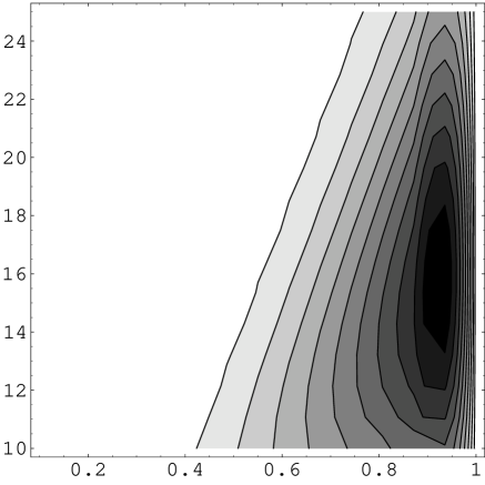
Figure 30: Contour of $(-1/2){\tilde{p}}^{3}W_{4}({\tilde{p}},z)F^{-}({\tilde{p}},z)$(linear suppression, Fig.17). $\Lambda=100,\ \omega=10,\ T=1$ . $1.0001/\omega\leq z\leq 0.9999/T,\ \mu=\Lambda T/\omega\leq{\tilde{p}}\leq 25$.

Figure 31: Minimal Area Curve ${\tilde{p}}(z)$, (117). ${\tilde{p}}(1.0)=30.0$, ${\tilde{p}}^{\prime}(1.0)=10.0$. Horizontal axis: 0.0001$\leq$ z $\leq$ 1.0 ; Vertical axis: $0.0\leq{\tilde{p}}\leq 30$.

12 App. D: Numerical Evaluation of Scaling Laws: $E_{Cas}$ (50), $E_{Cas}^{RS}$ (52), and $E_{Cas}^{W}$ (92)

In the text, (regularized) Casimir energy is numerically calculated in three ways: 1) Original version (Rectangle-region integral), 2) Restricted-region integral ( Randall-Sundrum type ), 3) Weighted version. The final expressions show the scaling behaviors about the boundary (extra-space) parameters $T$ , $\omega$ and the 4D momentum cut-off $\Lambda$. The results are crucial for the present conclusion. Hence we explain here how the numerical results are obtained.

First, let us take the un-weighted case with the rectangle integral-region (original form) of Casimir energy (49).

$$-E_{Cas}^{\Lambda,\mp}(\omega,T)=\frac{2\pi^{2}}{(2\pi)^{4}}\int_{\mu}^{\Lambda}d{\tilde{p}}\int_{1/\omega}^{1/T}dz\leavevmode\nobreak\ {\tilde{p}}^{3}F^{\mp}({\tilde{p}},z){\quad,}$$

$$F^{\mp}({\tilde{p}},z)=\frac{2}{(\omega z)^{3}}\int_{\tilde{p}}^{\Lambda}{\tilde{k}}\leavevmode\nobreak\ G^{\mp}_{k}(z,z)d{\tilde{k}}{\quad.}$$ (153)

where $G^{\mp}_{k}$ is explicitly given in (44). The integral region is graphically shown, in Fig.7, as the rectangle ($[1/\omega,1/T]\times[\mu=\Lambda T/\omega,\Lambda]$). The graphs of the integrand of (153), $(-1/2){\tilde{p}}^{3}F({\tilde{p}},z)$, are shown for $(T,\omega,\Lambda)=(1,10^{4},10^{4})\mbox{[}Fig.\ref{p3FmL10000}],(1,10^{4},2\times 10^{4})\mbox{[}Fig.\ref{p3FmL20000}],(1,10^{4},4\times 10^{4})\mbox{[}Fig.\ref{p3FmL40000}],$ in the text. From the behaviors we can expect $E_{Cas}^{\Lambda}(\omega,T)$, (153), leadingly behaves as $\Lambda^{5}/T$, because the depth of the valley, shown in Fig.8-10, proportional to $\Lambda^{4}$ and their behaviors are monotonous (except near the boundaries $z=1/\omega$ and $1/T$) along the extra axis. It is confirmed by directly evaluating (153) numerically (the numerical integral in [49]). We plot the numerical results in Fig.32 for various $\Lambda$’s with fixed $(T,\omega)$, and in Fig.33 for various $T$’s with fixed $(\omega,\Lambda)$.

Figure 32: Casimir Energy $E_{Cas}^{\Lambda,-}$ of (153) for various $\Lambda$. $T=1,\ \omega=10^{4}$. Horizontal axis: $\ln\Lambda$ ($\Lambda=10^{4}\times(1,2,4,8,16)$), Vertical Axis: $-\ln(|2^{3}\pi^{2}\times(1/2)E_{Cas}^{\Lambda,-}|)$.

Figure 33: Casimir Energy $E_{Cas}^{\Lambda,-}$ of (153) for various $T$. $\omega=10^{4},\ \Lambda=2\times 10^{4}$. Horizontal axis: $\ln T$ ($T=(1,2,4,8,16)$), Vertical Axis: $\ln(|2^{3}\pi^{2}\times(1/2)E_{Cas}^{\Lambda,-}|)$.

Furthermore we have confirmed sufficient $\omega$-indepedence for the region $T=1,\omega=10^{3}\times(1,2,4,8,16),\Lambda=10^{4}\times(2,4)$. Let us fit $E_{Cas}^{\Lambda}(\omega,T)$ from the above numerical results. First we can regard it as the function of one massive parameter $\Lambda$, and two massless parameters $\Lambda/T$ and $\Lambda/\omega$. From the linear dependences in Fig.32 and Fig.33 we may put

$$E_{Cas}^{\Lambda}(\omega,T)=\frac{\Lambda^{5}}{T}(a_{1}+a_{2}\ln\frac{\Lambda}{T}+a_{3}\ln\frac{\Lambda}{\omega}){\quad.}$$ (154)

From the $\omega$-independence, we take $a_{3}=0$. From the numerical results, the best fit is given by (Manipulating Numerical Data in [49])

$$E^{\Lambda,-}_{Cas}(\omega,T)=\frac{1}{8\pi^{2}}\times\left[-0.02500\frac{\Lambda^{5}}{T}(1-4.685\times 10^{-9}\ln\frac{\Lambda}{T})\right]{\quad.}$$ (155)

From the precision of the numerical integral, we may safely regard the log term in (155) vanishing ($a_{2}=0$). Finally we obtain (50).

For the restricted region case, (52), we do the numerical integral of the following expression.

$$-E^{-RS}_{Cas}(\omega,T)=\frac{2\pi^{2}}{(2\pi)^{4}}\int_{\mu}^{\Lambda}dq\int_{1/\omega}^{\Lambda/\omega q}dz\leavevmode\nobreak\ q^{3}F^{-}(q,z)=\frac{2\pi^{2}}{(2\pi)^{4}}\int_{1/\omega}^{1/T}du\int_{\mu}^{\Lambda/\omega u}d{\tilde{p}}\leavevmode\nobreak\ {\tilde{p}}^{3}F^{-}({\tilde{p}},u){\quad,}$$ (156)

where $\mu=\Lambda T/\omega$. We plot the results, in Fig.34, for various $\Lambda$ with fixed $(\omega,T)$ and in Fig.35, for vaious $\omega$ with fixed $(T,\Lambda)$.

Figure 34: Casimir Energy $E_{Cas}^{-RS}$ of (156) for various $\Lambda$ with fixed $(\omega=10^{3},T=1)$. Horizontal axis: $\ln\Lambda$ ($\Lambda=(1,2,4,8,16)\times 10^{4}$), Vertical Axis: $\ln(|2^{3}\pi^{2}\times\frac{1}{2}E_{Cas}^{-RS}|)$. The results are placed on a straight line with the slope 5 for different $\Lambda$’s.

Figure 35: Casimir Energy $E_{Cas}^{-RS}$ of (156) for various $\omega$ with fixed $(T=1,\Lambda=2\times 10^{4})$. Horizontal axis: $\ln\omega$ ($\omega=(1,2,4,8,16)\times 10^{2}$), Vertical Axis: $\ln(|2^{3}\pi^{2}\times\frac{1}{2}E_{Cas}^{-RS}|)$. The results are placed on a straight line with the slope -1 for different $\omega$’s.

Furthermore we have confirmed T-independence for $T=(1,2,3)$ with $(\omega=10^{4},\Lambda=2\times 10^{4})$ and for $T=(1,2,3,4,8,16)$ with $(\omega=10^{3},\Lambda=2\times 10^{4})$. From the straight line behaviors and the T-independence, we can safely fit the curve as $E_{Cas}^{-RS}=(\Lambda^{5}/\omega)(b_{1}+b_{2}\ln(\Lambda/T)+b_{3}\ln(\Lambda/\omega)),b_{2}=0$. The best fit is given by

$$2^{3}\pi^{2}E_{Cas}^{-RS}(\omega,T)=\frac{\Lambda^{5}}{\omega}\left((-1.59,-1.56)\times 10^{-2}+(-1.41,-1.97)\times 10^{-4}\leavevmode\nobreak\ \ln(\Lambda/\omega)\right){\quad.}$$ (157)

The first component of the above coefficients comes from Fig.34 data, the second one from Fig.35 data. The "width" of the coefficient-values tells us the first-term coefficient has the significant digit number 2, while the second-term one has the number 1. In the text, we take the average values (52).

Finally we explain the weighted case (78) taking the elliptic type, $W_{1}$, as an example.

$$-E^{-\leavevmode\nobreak\ W_{1}}_{Cas}(\omega,T)\equiv\int_{{\tilde{p}}\leq\Lambda}\frac{d^{4}p_{E}}{(2\pi)^{4}}\int_{1/\omega}^{1/T}dz\leavevmode\nobreak\ W_{1}({\tilde{p}},z)F^{-}({\tilde{p}},z){\quad,}$$

$$(N_{1})^{-1}{\rm e}^{-(1/2){\tilde{p}}^{2}/\omega^{2}-(1/2)z^{2}T^{2}}\equiv W_{1}({\tilde{p}},z),\ N_{1}=1.711/8\pi^{2}{\quad,}$$ (158)

where the UV cut-off $\Lambda$ is introduced to see the scaling behavior. In Fig.36, we show the numerical results of $E^{-W_{1}}_{Cas}(\omega,T)$ for different $\Lambda$’s with fixed $(T,\omega)$.

Figure 36: Casimir Energy $E_{Cas}^{-W_{1}}$ of (158) for various $\Lambda$ with fixed $(T=1,\omega=10^{3})$(RightDown) and $(T=0.01,\omega=10^{2})$(LeftUp). Horizontal axis: $\ln\Lambda$ ($\Lambda=10^{3}\times(1,2,4,8,16)$ and $10^{4}\times(1,2,4,8,16)$), Vertical Axis: $-\ln|2^{3}\pi^{2}(\frac{N_{1}}{2})E_{Cas}^{-\leavevmode\nobreak\ W_{1}}|$.

The two lines both are straight ones with the slope -1. For the T-dependence (with fixed $(\omega,\Lambda)$) and $\omega$-dependence (with fixed $(T,\Lambda)$) we show them in Fig.37 and in Fig.38, respectively.

Figure 37: Casimir Energy $E_{Cas}^{-W_{1}}$ of (158) for various $T$ with fixed $(\Lambda=2\times 10^{4},\omega=10^{3})$. Horizontal axis: $\ln\leavevmode\nobreak\ T$ ($T=(1,1/2,1/4,1/8,1/16)$), Vertical Axis: $-\ln|2^{3}\pi^{2}(\frac{N_{1}}{2})E_{Cas}^{-\leavevmode\nobreak\ W_{1}}|$.

Figure 38: Casimir Energy $E_{Cas}^{-W_{1}}$ of (158) for various $\omega$ with fixed $(\Lambda=8\times 10^{4},T=1)$. Horizontal axis: $\ln\leavevmode\nobreak\ \omega$ ($\omega=10^{2}\times(4,8,16,32,64,128)$), Vertical Axis: $-\ln|2^{3}\pi^{2}(\frac{N_{1}}{2})E_{Cas}^{-\leavevmode\nobreak\ W_{1}}|$.

They are straight lines with slopes +1 and -4, respectively. From the straight-lines behavior of Fig.36-38, we can safely fit the curve as $E_{Cas}^{-W1}=(\omega^{4}\Lambda/T)(c_{1}+c_{2}\ln(\Lambda/\omega)+c_{3}\ln(\Lambda/T))$. The best fit is given by

$$(2^{3}\pi^{2}N_{1}/2)\times E_{Cas}^{-W_{1}}(\omega,T)=\frac{\omega^{4}}{T}\Lambda\left(-1.04-0.11\leavevmode\nobreak\ \ln\frac{\Lambda}{\omega}+0.099\leavevmode\nobreak\ \ln\frac{\Lambda}{T}\right){\quad.}$$ (159)

Taking into account the present precision, we take $c_{1}=1.04\times(2/1.711)=1.22,\ c_{2}=0.11\times(2/1.711)=0.13,\ c_{3}=-0.099\times(2/1.711)=-0.12$ in the text. As for other types of $W$’s, the best fit scaling behaviors are listed in (92) of the text.

13 App. E.  Normalization Constants of Weight Functions (78)

In Sec.6, we introduce the weight function $W$ to evaluate the Casimir energy. For the comparison between the Casimir energy values obtained by different $W$’s, the normalization constants are important. The normalization constants $N_{i}$’s (78) are defined by the following condition:

$$\int_{\mu=\Lambda T/\omega<{\tilde{p}}<\Lambda}\frac{d^{4}p}{(2\pi)^{4}}\int_{1/\omega}^{1/T}dz\leavevmode\nobreak\ W_{i}({\tilde{p}},z)=\frac{1}{8\pi^{2}}\frac{\omega^{4}}{T}\int_{\Lambda T/\omega^{2}}^{\Lambda/\omega}dx\int_{T/\omega}^{1}dw\leavevmode\nobreak\ x^{3}W_{i}({\tilde{p}}=\omega x,z=w/T)$$

$$\equiv\frac{\omega^{4}}{T}{\quad,}\quad\quad\Lambda\gg\omega\gg T{\quad,}$$ (160)

For the ends of the integral-regions, we practically may take $\frac{\Lambda}{\omega}=\infty$ and $\frac{T}{\omega}=0$ except for $W_{2}$ and $W_{3}$. As for the starting end of $x$-integral, we have two choices depending on what range of the value $\omega$ is considered ( (A) $\omega\sim\sqrt{\Lambda T}$, (B) $\omega\gg\sqrt{\Lambda T}$ (C) $\omega\ll\sqrt{\Lambda T}$ ) in the numerical data-taking. They are explicitly given by

(A) $\omega\sim\sqrt{\Lambda T}$ (geometrically averaged point)
In this case, we take $\frac{\Lambda T}{\omega^{2}}=1,\frac{T}{w}=0,\frac{\Lambda}{\omega}=\infty$ in (160).

$$8\pi^{2}N_{1}=\frac{3}{\sqrt{{\rm e}}}\int_{0}^{1}dw\leavevmode\nobreak\ {\rm e}^{-w^{2}/2}=1.557{\quad,}\quad 8\pi^{2}N_{1b}=\frac{3}{\sqrt{{\rm e}}}=\int_{1}^{\infty}dx\leavevmode\nobreak\ x^{3}{\rm e}^{-x^{2}/2}=1.820{\quad,}$$

$$8\pi^{2}N_{2}=\int_{1}^{\infty}dx\int_{T/\omega}^{1}\leavevmode\nobreak\ dwx^{3}{\rm e}^{-xw}=2(\frac{\omega}{T})^{3}{\quad,}$$

$$8\pi^{2}N_{3}=\int_{1}^{\infty}dx\int_{T/\omega}^{1}\leavevmode\nobreak\ dwx^{3}{\rm e}^{-x^{2}w^{2}/2}=\frac{2}{3}(\frac{\omega}{T})^{3}{\quad,}$$

$$8\pi^{2}N_{4}=\int_{1}^{\infty}dx\int_{0}^{1}dw\leavevmode\nobreak\ x^{3}{\rm e}^{-x^{2}/2w^{2}}=0.3222{\quad,}\quad 8\pi^{2}N_{5}=\int_{1}^{\infty}dx\int_{0}^{1}dw\leavevmode\nobreak\ x^{3}{\rm e}^{-x/w^{2}}=0.6342{\quad,}$$

$$8\pi^{2}N_{6}=\int_{1}^{\infty}dx\int_{0}^{1}dw\leavevmode\nobreak\ x^{3}{\rm e}^{-x^{2}/2w}=0.5521{\quad,}\quad 8\pi^{2}N_{7}=\int_{1}^{\infty}dx\leavevmode\nobreak\ x^{3}{\rm e}^{-x^{4}/2}=\frac{1}{2\sqrt{{\rm e}}}=0.3033{\quad,}$$

$$8\pi^{2}N_{8}=\frac{3}{\sqrt{{\rm e}}}\int_{0}^{1}dw\leavevmode\nobreak\ {\rm e}^{-1/2w^{2}}=0.3800{\quad,}\quad 8\pi^{2}N_{47}=\int_{1}^{\infty}dx\int_{0}^{1}dw\leavevmode\nobreak\ x^{3}{\rm e}^{-x^{2}(x^{2}+1/w^{2})/2}=0.03893{\quad,}$$

$$8\pi^{2}N_{56}=\int_{1}^{\infty}dx\int_{0}^{1}dw\leavevmode\nobreak\ x^{3}{\rm e}^{-(x/w)(x+1/w)/2}=0.1346{\quad,}$$

$$8\pi^{2}N_{88}=\int_{1}^{\infty}dx\int_{0}^{1}dw\leavevmode\nobreak\ x^{3}{\rm e}^{-(1/2)(x^{2}+1/w^{2})^{2}}=0.005006{\quad,}$$

$$8\pi^{2}N_{9}=\int_{1}^{\infty}dx\int_{0}^{1}dw\leavevmode\nobreak\ x^{3}{\rm e}^{-(1/2)(x+1/w)^{2}}=0.03921{\quad,}$$ (161)

(B) $\omega\gg\sqrt{\Lambda T}$
In this case, we take $\frac{\Lambda T}{\omega^{2}}=0,\frac{T}{w}=0,\frac{\Lambda}{\omega}=\infty$ in (160).

$$8\pi^{2}N_{1}=2\times\int_{0}^{1}dw\leavevmode\nobreak\ {\rm e}^{-w^{2}/2}=1.711{\quad,}\quad 8\pi^{2}N_{1b}=\int_{0}^{\infty}dx\leavevmode\nobreak\ x^{3}{\rm e}^{-x^{2}/2}=2{\quad,}$$

$$8\pi^{2}N_{2}=\int_{0}^{\infty}dx\int_{T/\omega}^{1}\leavevmode\nobreak\ dwx^{3}{\rm e}^{-xw}=2(\frac{\omega}{T})^{3}{\quad,}$$

$$8\pi^{2}N_{3}=\int_{0}^{\infty}dx\int_{T/\omega}^{1}\leavevmode\nobreak\ dwx^{3}{\rm e}^{-x^{2}w^{2}/2}=\frac{2}{3}(\frac{\omega}{T})^{3}{\quad,}$$

$$8\pi^{2}N_{4}=\int_{0}^{\infty}dx\int_{0}^{1}dw\leavevmode\nobreak\ x^{3}{\rm e}^{-x^{2}/2w^{2}}=\frac{2}{5}{\quad,}\quad 8\pi^{2}N_{5}=\int_{0}^{\infty}dx\int_{0}^{1}dw\leavevmode\nobreak\ x^{3}{\rm e}^{-x/w^{2}}=\frac{2}{3}{\quad,}$$

$$8\pi^{2}N_{6}=\int_{0}^{\infty}dx\int_{0}^{1}dw\leavevmode\nobreak\ x^{3}{\rm e}^{-x^{2}/2w}=\frac{2}{3}{\quad,}\quad 8\pi^{2}N_{7}=\int_{0}^{\infty}dx\leavevmode\nobreak\ x^{3}{\rm e}^{-x^{4}/2}=\frac{1}{2}{\quad,}$$

$$8\pi^{2}N_{8}=2\times\int_{0}^{1}dw\leavevmode\nobreak\ {\rm e}^{-1/2w^{2}}=0.4177{\quad,}$$

$$8\pi^{2}N_{47}=\int_{0}^{\infty}dx\int_{0}^{1}dw\leavevmode\nobreak\ x^{3}{\rm e}^{-x^{2}(x^{2}+1/w^{2})/2}=0.1028{\quad,}$$

$$8\pi^{2}N_{56}=\int_{0}^{\infty}dx\int_{0}^{1}dw\leavevmode\nobreak\ x^{3}{\rm e}^{-(x/w)(x+1/w)/2}=0.1779{\quad,}$$

$$8\pi^{2}N_{88}=\int_{0}^{\infty}dx\int_{0}^{1}dw\leavevmode\nobreak\ x^{3}{\rm e}^{-(1/2)(x^{2}+1/w^{2})^{2}}=0.01567{\quad,}$$

$$8\pi^{2}N_{9}=\int_{0}^{\infty}dx\int_{0}^{1}dw\leavevmode\nobreak\ x^{3}{\rm e}^{-(1/2)(x+1/w)^{2}}=0.05320{\quad,}$$ (162)

In the text, we take the case (B).

(C) $\omega\ll\sqrt{\Lambda T}$
In this case, we may take $\frac{\Lambda T}{\omega^{2}}=0,\frac{T}{w}=0,\frac{\Lambda}{\omega}=\infty$ in (160). This is the same as the case (B). In Sec.8, we apply the results to the cosmological constant or the dark energy. We take there $\Lambda=10^{28}$ eV, $\omega=10^{-3}$ eV and $T=10^{-20}$ eV.

14 Acknowledgment

Parts of the content of this work have been already presented at the international conference on "Progress of String Theory and Quantum Field Theory" (07.12.7-10, Osaka City Univ., Japan), 63rd Meeting of Japan Physical Society (08.3.22-26,Kinki Univ.,Osaka,Japan), Summer Institute 2008 (08.8.10-17, Chi-Tou, Taiwan), the international conference on "Particle Physics, Astrophysics and Quantum Field Theory"(08.11.27-29, Nanyang Executive Centre, Singapore), 1st Mediterranean Conference on Classical and Quantum Gravity (09.9.14-18,Greece) and the international workshop on "Strong Coupling Gauge Theories in LHC Era" (09.12.8-11, Nagoya, Japan). The author thanks T. Appelquist (Yale Univ.), S.J. Brodsky (SLAC), K. Fujikawa (Nihon Univ.), T. Inagaki (Hiroshima Univ.), K. Kanaya (Tsukuba Univ.), T. Kugo (Kyoto Univ.), S. Moriyama (Nagoya Univ.), N. Sakai (Tokyo Women’s Univ.), M. Tanabashi (Nagoya Univ.) and H. Terao (Nara Women’s Univ.) for useful comments on the occasions.

References

[1] M. Bordag, U. Mohideen and V.M. Mostepanenko, Phys.Rept.353(2001),1,arXiv:quant-ph/0106045
K. A. Milton, J. Phys. A37(2004)R209, arXiv:hep-th/0406024
P. A. Martin and P. R. Buenzli, Acta Phys Polonica B 37(2006)2503, arXiv:cond-mat/0602559
[2] Th. Kaluza, Sitzungsberichte der K.Preussischen Akademite der
Wissenschaften zu Berlin. p966 (1921)
[3] O. Klein, Z. Physik 37 895 (1926)
[4] M. B. Green, J. H. Schwartz and E. Witten, Superstring theory, Vol.I and II,
Cambridge Univ. Press, c1987, Cambridge
J. Polchinski, STRING THEORY, Vol.I and II, Cambridge Univ. Press, c1998, Cambridge
[5] T. Appelquist and A. Chodos, Phys.Rev.D28(1983)772
T. Appelquist and A. Chodos, Phys.Rev.Lett.50(1983)141
[6] S. Ichinose, Phys.Lett.152B(1985),56
[7] W. Goldberger and M. Wise, Phys.Rev.Lett.83(1999)4922
[8] W. Goldberger and M. Wise, Phys.Lett.B475(2000)275
[9] D. Toms, Phys.Lett.B484(2000)149
[10] W. Goldberger and M. Wise, Phys.Rev.D65(2002)025011
[11] W. Goldberger and I. Rothstein, Phys.Lett.B491(2000)339
[12] A. Flachi and D. Toms, Nucl.Phys.B610(2001)144
[13] J. Garriga, O. Pujolas, and T. Tanaka, Nucl.Phys.B605(2001)192
[14] E. Pontón and E. Poppitz, J. High Energy Phys.0106(2001)019
[15] A. Flachi, J. Garriga, O. Pujola’s, and T. Tanaka, J. High Energy Phys.08(2003)053
[16] A. Flachi and O. Pujola’s, Phys.Rev.D68(2003)025023
[17]L. Suskind and E. Witten, "The Holographic Bound in Anti-de Sitter Space", arXiv:hep-th/9805114
[18]M. Henningson and K. Skenderis, JHEP 9807(1998)023, arXiv:hep-th/9806087
M. Henningson and K. Skenderis, Fortsch.Phys. 48(2000)125, arXiv:hep-th/9812032
[19]K. Skenderis and P.K. Townsend, Phys.Lett.B468(1999)46, arXiv:hep-th/9909070
[20]O. DeWolfe, D.Z. Freedman, S.S. Gubser and A. Karch, Phys.Rev.D62(2000) 046008,
arXiv:hep-th/9909134
[21]D.Z. Freedman, S.S. Gubser, K. Pilch and N.P. Warner, Adv.Theor.Math.Phys.3(1999)363,
arXiv:hep-th/9904017
[22]J. de Boer, E. Verlinde and H. Verlinde, JHEP 0008(2000)003, arXiv:hep-th/9912012
[23]J.M. Maldacena, Adv.Theor.Math.Phys.2(1998)231 [Int. J. Theor. Phys.38(1999)1113],
arXiv:hep-th/9711200
[24]S. S. Gubser, I. R. Klebanov and A. M. Polyakov, Phys.Lett.B428(1998)105, arXiv:hep-th/9802109
[26] S. Ichinose, Prog.Theor.Phys.121(2009)727, ArXiv:0801.3064v8[hep-th].
[27]S. Ichinose, "Casimir Energy of the Universe and New Regularization of Higher Dimensional
Quantum Field Theories", First Mediterranean Conference on Classical and Quantum Gravity
(09.9.14-18, Kolymbari, Crete, Greece), to appear in the proceedings. ArXiv:1001.0222[hep-th].
[28]S. Ichinose, "New Regularization in Extra Dimensional Model and Renormalization Group
Flow of the Cosmological Constant", Int. Workshop on ’Strong Coupling Gauge Theories
in LHC Era’(09.12.8-11, Nagoya Univ., Nagoya, Japan).
[29] L. Randall and M.D. Schwartz, JHEP 0111 (2001) 003, hep-th/0108114
[30] J. Schwinger, Phys.Rev.82(1951)664
[31] S. Ichinose and A. Murayama, Phys.Rev.D76(2007)065008, hep-th/0703228
[32] S. Ichinose, Class.Quantum.Grav.18(2001)421, hep-th/0003275
[33] S. Ichinose, "Casimir and Vacuum Energy of 5D Warped System and Sphere Lattice Regularization",
Proc. of VIII Asia-Pacific Int. Conf. on Gravitation and Astrophysics
(ICGA8,Aug.29-Sep.1,2007,Nara Women’s Univ.,Japan),Press Section p36-39, arXiv:/0712.4043
[34] S. Ichinose, "Casimir Energy of 5D Electro-Magnetism and Sphere Lattice Regularization",
Int.Jour.Mod.Phys.23A(2008)2245-2248,
Proc. of Int. Conf. on Prog. of String Theory and Quantum Field Theory
(Dec.7-10,2007,Osaka City Univ.,Japan), arXiv:/0804.0945
[36] S. Ichinose and A. Murayama, Nucl.Phys.B710(2005)255, hep-th/0401011
[37] T. Yoneya, Duality and Indeterminacy Principle in String Theory in "Wandering in the Fields",
eds. K. Kawarabayashi and A. Ukawa (World Scientific,1987), p.419
T. Yoneya, String Theory and Quantum Gravity in "Quantum String Theory",
eds. N. Kawamoto and T. Kugo (Springer,1988), p.23
T. Yoneya, Prog.Theor.Phys.103(2000)1081
[38] S. Ichinose, hep-th/0012255, US-00-11, 2000,
"Pole Solution in Six Dimensions and Mass Hierarchy"
[39] S. Ichinose, Proc. of 10th Tohwa Int. Symp. on String Thery (Jul.3-7, 2001,
Tohwa Univ., Minerva Hall, Fukuoka, Japan), ed. H. Aoki and T. Tada,
C2002, AIP Conf. Proc. 607, American Inst. Phys., Melville, New York, p307
[40] S. Ichinose, Nucl.Phys.B231(1984)335
[41] P.A.M. Dirac,
Nature 139(1937)323; Proc.Roy.Soc.A165(1938)199; "Directions in Physics", John Wiley & Sons, Inc.,
New York, 1978
[42] A.M. Polyakov, "Phase Transition And The Universe", Sov.Phys.Usp.25(1982)187
[Usp.Fiz.Nauk.136(1982)538]
[43] S. Ichinose, Nucl.Phys.B457(1995)688
[44] P. Hor̆ava, "Membranes at Quantum Criticality", arXiv:hep-th/0812.4287
[45] P. Hor̆ava, "Quantum Gravity at a Lifshitz Point", arXiv:hep-th/0901.3775
[46] E. M. Lifshitz, Zh. Eksp. Theor. Fiz.11(1941)255,269
[47] C. Itzykson and J. B. Zuber, Quantum Field Theory, C1980, McGraw-Hill Inc.,New York
[48] A. Zee, "Quantum Field Theory in A Nutshell", C2003, Princeton Univ. Press, Princeton
[49] S. Wolfram, The Mathematica Book, 4th ed., Wolfram Media/Cambridge University Press, c1999