Thermodynamics and Finite size scaling in Scalar Field Theory

Debasish Banerjee debasish@theory.tifr.res.in Department of Theoretical Physics, Tata Institute of Fundamental Research,
Homi Bhabha Road, Mumbai 400005, India.
   Saumen Datta saumen@theory.tifr.res.in Department of Theoretical Physics, Tata Institute of Fundamental Research,
Homi Bhabha Road, Mumbai 400005, India.
   Sourendu Gupta sgupta@tifr.res.in Department of Theoretical Physics, Tata Institute of Fundamental Research,
Homi Bhabha Road, Mumbai 400005, India.

I Introduction

In this work we consider the 1-component real scalar ϕ4superscriptitalic-ϕ4\phi^{4} theory in 4 space-time dimensions on the lattice and investigate the finite size scaling of thermodynamic quantities to study whether the thermodynamic limit is attained. The results are obtained for the symmetric phase of the theory.

II Thermodynamic set up

The thermal expectation value of an operator 𝒪𝒪{\cal{O}} is

𝒪(φ)=1𝒵(β)𝒟φeβH𝒪(φ)delimited-⟨⟩𝒪𝜑1𝒵𝛽𝒟𝜑superscript𝑒𝛽𝐻𝒪𝜑\langle{\cal{O}(\varphi)}\rangle=\frac{1}{{\cal{Z}}(\beta)}\int{\cal D}\varphi e^{-\beta H}{\cal{O(\varphi)}} (1)

where 𝒵(β)𝒵𝛽{\cal{Z}}(\beta) is the partition function. For our finite temperature study, we have kept the temporal side fixed at T=β1=(Ntat)1𝑇superscript𝛽1superscriptsubscript𝑁𝑡subscript𝑎𝑡1T=\beta^{-1}=(N_{t}a_{t})^{-1} and varied the spatial extent L=Nsas𝐿subscript𝑁𝑠subscript𝑎𝑠L=N_{s}a_{s} by going to higher values of LT𝐿𝑇LT to examine the thermodynamic limit. Energy density E𝐸E and pressure P𝑃P are obtained by the following derivatives of the partition function: E=T2/Vln𝒵/T|V=1/(Ns3as3Nt)ln𝒵/at|V𝐸evaluated-atsuperscript𝑇2𝑉𝒵𝑇𝑉evaluated-at1superscriptsubscript𝑁𝑠3superscriptsubscript𝑎𝑠3subscript𝑁𝑡𝒵subscript𝑎𝑡𝑉E=T^{2}/V\left.\partial\ln{\cal{Z}}/\partial T\right|_{V}=-1/(N_{s}^{3}a_{s}^{3}N_{t})\left.\partial\ln{\cal{Z}}/\partial a_{t}\right|_{V} and P=Tln𝒵/V|T=1/(3Ns3as2Ntat)ln𝒵/as|T𝑃evaluated-at𝑇𝒵𝑉𝑇evaluated-at13superscriptsubscript𝑁𝑠3superscriptsubscript𝑎𝑠2subscript𝑁𝑡subscript𝑎𝑡𝒵subscript𝑎𝑠𝑇P=T\left.\partial\ln{\cal{Z}}/\partial V\right|_{T}=1/(3N_{s}^{3}a_{s}^{2}N_{t}a_{t})\left.\partial\ln{\cal{Z}}/\partial a_{s}\right|_{T} where assubscript𝑎𝑠a_{s} and atsubscript𝑎𝑡a_{t} are the lattice spacings along the spatial and temporal directions.
The continuum Euclidean action for the scalar ϕ4superscriptitalic-ϕ4\phi^{4} theory is

S[ϕ]=𝑑td3x{12μϕ(x)μϕ(x)+12m02ϕ(x)2+g04!ϕ(x)4}𝑆delimited-[]italic-ϕdifferential-d𝑡superscript𝑑3𝑥12subscript𝜇italic-ϕ𝑥subscript𝜇italic-ϕ𝑥12superscriptsubscript𝑚02italic-ϕsuperscript𝑥2subscript𝑔04italic-ϕsuperscript𝑥4\small{S[\phi]=\int dt\int d^{3}x\left\{\frac{1}{2}\partial_{\mu}\phi(x)\partial_{\mu}\phi(x)+\frac{1}{2}m_{0}^{2}\phi(x)^{2}+\frac{g_{0}}{4!}\phi(x)^{4}\right\}} (2)

The following redefinitions are made to trade off the set of couplings (g0,m0subscript𝑔0subscript𝑚0g_{0},m_{0}) for (κ,λ𝜅𝜆\kappa,\lambda):

κ𝜅\displaystyle\kappa =\displaystyle= 12λ3ξ+ξ3+((atm0)2/2)ξ3;κt=κsξ2=κξ3;12𝜆3𝜉superscript𝜉3superscriptsubscript𝑎𝑡subscript𝑚022superscript𝜉3subscript𝜅𝑡subscript𝜅𝑠superscript𝜉2𝜅superscript𝜉3\displaystyle\frac{1-2\lambda}{3\xi+\xi^{3}+((a_{t}m_{0})^{2}/2)\xi^{3}};~{}~{}\kappa_{t}=\kappa_{s}\xi^{2}=\kappa\xi^{3};
λ𝜆\displaystyle\lambda =\displaystyle= g024ξ3κ2;ϕ^=atϕκ;m^0=atm0formulae-sequencesubscript𝑔024superscript𝜉3superscript𝜅2^italic-ϕsubscript𝑎𝑡italic-ϕ𝜅subscript^𝑚0subscript𝑎𝑡subscript𝑚0\displaystyle\frac{g_{0}}{24}\xi^{3}\kappa^{2};\hat{\phi}=a_{t}\frac{\phi}{\sqrt{\kappa}};~{}~{}\hat{m}_{0}=a_{t}m_{0} (3)

where ξ=as/at𝜉subscript𝑎𝑠subscript𝑎𝑡\xi=a_{s}/a_{t} is the anisotropy parameter. This yields the conventional form of the action for doing simulations:

S[ϕ^]𝑆delimited-[]^italic-ϕ\displaystyle S[\hat{\phi}] =\displaystyle= xα{κsi=13ϕ^(xα+ai)ϕ^(xα)κtϕ^(xα+at)ϕ^(xα).\displaystyle\sum_{x_{\alpha}}\Bigl{\{}-\kappa_{s}\sum_{i=1}^{3}\hat{\phi}(x_{\alpha}+a_{i})\hat{\phi}(x_{\alpha})-\kappa_{t}\hat{\phi}(x_{\alpha}+a_{t})\hat{\phi}(x_{\alpha})\Bigr{.} (4)
+.ϕ^(xα)2+λ(ϕ^(xα)21)2}\displaystyle\qquad+\Bigl{.}\hat{\phi}(x_{\alpha})^{2}+\lambda(\hat{\phi}(x_{\alpha})^{2}-1)^{2}\Bigr{\}}

Since our simulations are on lattices with ξ=1𝜉1\xi=1, we calculate the relevant thermodynamic expressions for anisotropic lattices and then set the spacings to be equal. We renormalise the pressure to be zero at T=0𝑇0T=0 by subtracting the corresponding zero temperature operators from their finite temperature counterparts. This procedure is adopted to renormalise all the operators appearing in the other thermodynamic quantities as well and is denoted by adding the subscript “subt” to the operators. Finally, the expressions for the energy density E𝐸E, pressure P𝑃P and E3P𝐸3𝑃E-3P in this formulation is:

Eat4𝐸superscriptsubscript𝑎𝑡4\displaystyle Ea_{t}^{4} =\displaystyle= 1ξ3{ξSξ|atsubt+atSat|ξsubt}1superscript𝜉3𝜉subscriptdelimited-⟨⟩evaluated-at𝑆𝜉subscript𝑎𝑡𝑠𝑢𝑏𝑡subscriptdelimited-⟨⟩evaluated-atsubscript𝑎𝑡𝑆subscript𝑎𝑡𝜉𝑠𝑢𝑏𝑡\displaystyle\frac{1}{\xi^{3}}\left\{-\xi\left\langle\left.\frac{\partial S}{\partial\xi}\right|_{a_{t}}\right\rangle_{subt}+\left\langle\left.a_{t}\frac{\partial S}{\partial a_{t}}\right|_{\xi}\right\rangle_{subt}\right\}
Pat4𝑃superscriptsubscript𝑎𝑡4\displaystyle Pa_{t}^{4} =\displaystyle= 1ξ2Sξ|atsubt1superscript𝜉2subscriptdelimited-⟨⟩evaluated-at𝑆𝜉subscript𝑎𝑡𝑠𝑢𝑏𝑡\displaystyle-\frac{1}{\xi^{2}}\left\langle\left.\frac{\partial S}{\partial\xi}\right|_{a_{t}}\right\rangle_{subt}
(E3P)at4𝐸3𝑃superscriptsubscript𝑎𝑡4\displaystyle(E-3P)a_{t}^{4} =\displaystyle= 1ξ3atSat|ξsubt1superscript𝜉3subscriptdelimited-⟨⟩evaluated-atsubscript𝑎𝑡𝑆subscript𝑎𝑡𝜉𝑠𝑢𝑏𝑡\displaystyle\frac{1}{\xi^{3}}\left\langle\left.a_{t}\frac{\partial S}{\partial a_{t}}\right|_{\xi}\right\rangle_{subt} (5)

where bracketed quantities denote thermal averages. Note that the quantities Eat4𝐸superscriptsubscript𝑎𝑡4Ea_{t}^{4}Pat4𝑃superscriptsubscript𝑎𝑡4Pa_{t}^{4} and (E3P)at4𝐸3𝑃superscriptsubscript𝑎𝑡4(E-3P)a_{t}^{4} are all dimensionless quantities and will henceforth be referred to as E𝐸EP𝑃P and E3P𝐸3𝑃E-3P respectively in lattice units. The derivatives of the couplings of the theory with respect to ξ𝜉\xi are the anisotropy coefficients.
The renormalisation conditions for the theory involve fixing the 2- and 4-point renormalised vertex functions at zero momenta as follows:

m^R2=ΓR(2)(0);gR=ΓR(4)(0,0,0,0)formulae-sequencesuperscriptsubscript^𝑚𝑅2subscriptsuperscriptΓ2𝑅0subscript𝑔𝑅superscriptsubscriptΓ𝑅40000\hat{m}_{R}^{2}=-\Gamma^{(2)}_{R}(0);~{}g_{R}=-\Gamma_{R}^{(4)}(0,0,0,0) (6)
Refer to caption
Figure 1: The Feynman diagrams to 1-loop order that need to be calculated. The first set of diagrams is for the 2-point vertex function while the second one is for the 4-point vertex function.

Equation (5) requires evaluation of the following derivatives:

dκssubscript𝑑subscript𝜅𝑠\displaystyle d_{\kappa_{s}} =\displaystyle= atκsat|ξ;dκt=atκtat|ξ;dλ=atλat|ξformulae-sequenceevaluated-atsubscript𝑎𝑡subscript𝜅𝑠subscript𝑎𝑡𝜉subscript𝑑subscript𝜅𝑡evaluated-atsubscript𝑎𝑡subscript𝜅𝑡subscript𝑎𝑡𝜉subscript𝑑𝜆evaluated-atsubscript𝑎𝑡𝜆subscript𝑎𝑡𝜉\displaystyle\left.a_{t}\frac{\partial\kappa_{s}}{\partial a_{t}}\right|_{\xi};~{}d_{\kappa_{t}}=\left.a_{t}\frac{\partial\kappa_{t}}{\partial a_{t}}\right|_{\xi};~{}d_{\lambda}=\left.a_{t}\frac{\partial\lambda}{\partial a_{t}}\right|_{\xi} (7)
cκssubscript𝑐subscript𝜅𝑠\displaystyle c_{\kappa_{s}} =\displaystyle= κs|at;cκt=κt|at;cλ=λ|atformulae-sequenceevaluated-atsuperscriptsubscript𝜅𝑠subscript𝑎𝑡subscript𝑐subscript𝜅𝑡evaluated-atsuperscriptsubscript𝜅𝑡subscript𝑎𝑡subscript𝑐𝜆evaluated-atsuperscript𝜆subscript𝑎𝑡\displaystyle\left.\kappa_{s}^{\prime}\right|_{a_{t}};~{}~{}~{}~{}~{}c_{\kappa_{t}}=\left.\kappa_{t}^{\prime}\right|_{a_{t}};~{}~{}~{}~{}~{}~{}c_{\lambda}=\left.\lambda^{\prime}\right|_{a_{t}} (8)

where f=f/ξsuperscript𝑓𝑓𝜉f^{\prime}=\partial f/\partial\xi. The first three derivatives can be completely specified using β=atg0/at|ξ𝛽evaluated-atsubscript𝑎𝑡subscript𝑔0subscript𝑎𝑡𝜉\beta=a_{t}\left.\partial g_{0}/\partial a_{t}\right|_{\xi} and γ=atm0^2/at|ξ𝛾evaluated-atsubscript𝑎𝑡superscript^subscript𝑚02subscript𝑎𝑡𝜉\gamma=a_{t}\left.\partial\hat{m_{0}}^{2}/\partial a_{t}\right|_{\xi} functions. We have used the 1-loop expressions for the β𝛽\beta and γ𝛾\gamma functions of the lattice theory available in literature MM . The latter three involve the anisotropy coefficients g0=g0/ξ|atsuperscriptsubscript𝑔0evaluated-atsubscript𝑔0𝜉subscript𝑎𝑡g_{0}^{\prime}=\left.\partial g_{0}/\partial\xi\right|_{a_{t}} and (m0^2)=m0^2/ξ|atsuperscriptsuperscript^subscript𝑚02evaluated-atsuperscript^subscript𝑚02𝜉subscript𝑎𝑡(\hat{m_{0}}^{2})^{\prime}=\left.\partial\hat{m_{0}}^{2}/\partial\xi\right|_{a_{t}}, whose expressions do not exist in literature for this scalar theory. We have evaluated the anisotropy coefficients upto 1 loop order by summing the Feynman diagrams shown in fig 1 to be:

K(x)𝐾𝑥\displaystyle K(x) =\displaystyle= [(3m^R2+12)I04(2x)12I03(2x)I1(2x)]delimited-[]3superscriptsubscript^𝑚𝑅212superscriptsubscript𝐼042𝑥12superscriptsubscript𝐼032𝑥subscript𝐼12𝑥\displaystyle\left[(3\hat{m}_{R}^{2}+12)I_{0}^{4}(2x)-12I_{0}^{3}(2x)I_{1}(2x)\right]
(m^02)|atevaluated-atsuperscriptsuperscriptsubscript^𝑚02subscript𝑎𝑡\displaystyle\left.(\hat{m}_{0}^{2})^{\prime}\right|_{a_{t}} =\displaystyle= gR20x𝑑xe(m^R2+8)xK(x)subscript𝑔𝑅2superscriptsubscript0𝑥differential-d𝑥superscript𝑒superscriptsubscript^𝑚𝑅28𝑥𝐾𝑥\displaystyle\frac{g_{R}}{2}\int_{0}^{\infty}xdxe^{-(\hat{m}_{R}^{2}+8)x}K(x)
g0|atevaluated-atsuperscriptsubscript𝑔0subscript𝑎𝑡\displaystyle\left.g_{0}^{\prime}\right|_{a_{t}} =\displaystyle= 32gR20x2𝑑xex(m^R2+8)K(x)32superscriptsubscript𝑔𝑅2superscriptsubscript0superscript𝑥2differential-d𝑥superscript𝑒𝑥superscriptsubscript^𝑚𝑅28𝐾𝑥\displaystyle-\frac{3}{2}g_{R}^{2}\int_{0}^{\infty}x^{2}dxe^{-x(\hat{m}_{R}^{2}+8)}K(x) (9)

where In(x)subscript𝐼𝑛𝑥I_{n}(x) denotes the modified Bessel function of order n. The calculation of these coefficients was done using Mathematica which could handle large range of numbers, much beyond the capacity of usual C compilers. This was specially important since the numerical values depend on a delicate cancellation among Bessel functions. The anisotropy coefficients evaluated at the simulation points is listed in table 1.

III Numerical Methods

Table 1: Parameter values at each of the different points. gRsubscript𝑔𝑅g_{R} is calculated in 1 loop perturbation theory. For comparison, estimate of mass in 1 loop perturbation theory is also shown.
No. A B C D
κ𝜅\kappa 0.25160.25160.2516 0.25260.25260.2526 0.2534520.2534520.253452 0.254380.254380.25438
λ𝜆\lambda 0.0111530.0111530.011153 0.01170.01170.0117 0.01220.01220.0122 0.01340.01340.0134
gRsubscript𝑔𝑅g_{R} 3.17723.17723.1772 3.189553.189553.18955 3.164783.164783.16478 3.171083.171083.17108
ma𝑚𝑎ma 0.28530.28530.2853 0.23760.23760.2376 0.18970.18970.1897 0.14160.14160.1416
±0.0002plus-or-minus0.0002\pm 0.0002 ±0.0003plus-or-minus0.0003\pm 0.0003 ±0.0002plus-or-minus0.0002\pm 0.0002 ±0.0002plus-or-minus0.0002\pm 0.0002
ma𝑚𝑎ma (in 1 loop) 0.30120.30120.3012 0.25860.25860.2586 0.21720.21720.2172 0.18340.18340.1834
g0superscriptsubscript𝑔0g_{0}^{\prime} 1.93721.9372-1.9372 2.063482.06348-2.06348 2.164512.16451-2.16451 2.344492.34449-2.34449
(m0^2)superscriptsuperscript^subscript𝑚02(\hat{m_{0}}^{2})^{\prime} 0.3679010.3679010.367901 0.3697380.3697380.369738 0.3671930.3671930.367193 0.3681730.3681730.368173

A overrelaxation+Metropolis (OR+M) algorithm was used to generate the equilibrium configurations on which the operators were measured. The OR+M algorithm caused the correlation time at critical point to reduce by a factor of 10 compared to the Metropolis and the time to generate independent configurations was 0.40.40.4s. Configurations separated by 3τint3subscript𝜏𝑖𝑛𝑡3\tau_{int} were considered to be independent, where τintsubscript𝜏𝑖𝑛𝑡\tau_{int} was the Monte-Carlo time for the autocorrelation function to decay to 1/e1𝑒1/e. To check the accuracy of our program, simulations were done at (λ=0.275376,κ=0.288998formulae-sequence𝜆0.275376𝜅0.288998\lambda=0.275376,\kappa=0.288998) where we measured the vacuum expectation value of the ϕitalic-ϕ\phi field and its susceptibility, and compared it with the results obtained in balog .

The jackknife method was used to calculate the errors on the operators. It was checked that the block size used was much above the minimum bin size over which the variance showed a plateau.
Refer to caption
Refer to caption
Refer to caption
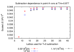
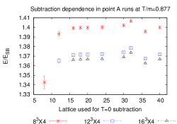
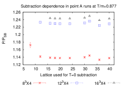
Figure 2: Comparison of different subtraction schemes on the E/ESB𝐸subscript𝐸𝑆𝐵E/E_{SB}, P/PSB𝑃subscript𝑃𝑆𝐵P/P_{SB} and (E3P)/T4𝐸3𝑃superscript𝑇4(E-3P)/T^{4} at point A

IV Physics Results

The simulations were done on Renormalisation Group (RG) trajectories of constant gRsubscript𝑔𝑅g_{R}. A point was chosen (κ=0.2516,λ=0.011153formulae-sequence𝜅0.2516𝜆0.011153\kappa=0.2516,\lambda=0.011153) where the scaling violations could be neglected lw1 . The physical mass was extracted non-perturbatively at this point A. Points B, C and D with cut-off effects 4/5454/52/3232/3 and 1/2121/2 of point A and lying on the same RG trajectory were first constructed within 1-loop perturbation theory and then non-perturbatively tuned to get the desired ma𝑚𝑎ma. The parameter details of the points are given in table 1.
Refer to caption
Refer to caption
Refer to caption
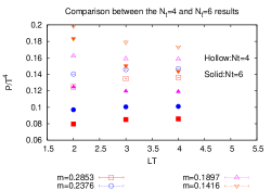
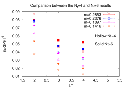
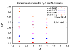
Figure 3: Scaling of the E/T4𝐸superscript𝑇4E/T^{4}, P/T4𝑃superscript𝑇4P/T^{4} and (E3P)/T4𝐸3𝑃superscript𝑇4(E-3P)/T^{4} for Nt=4subscript𝑁𝑡4N_{t}=4 and Nt=6subscript𝑁𝑡6N_{t}=6.

To estimate zero T subtraction, operators evaluated on lattices ranging from 404superscript40440^{4} till Ns4superscriptsubscript𝑁𝑠4N_{s}^{4} were subtracted from the corresponding operators evaluated on the Ns3×4superscriptsubscript𝑁𝑠34N_{s}^{3}\times 4 lattice at point A. The result is shown in fig 2. Our results indicate that a plateau is reached for all the thermodynamic quantities when the subtraction lattices used N4superscript𝑁4N^{4} are much greater than Ns4superscriptsubscript𝑁𝑠4N_{s}^{4} except for the runs at 324superscript32432^{4} and 364superscript36436^{4} which seem to give erratic results. We checked that the problem was not in the analysis. In what follows, we do not include these two sets in the discussion of the thermodynamic limit. The result of subtracting with a 404superscript40440^{4} lattice agrees with the results obtained by subtraction from the N4superscript𝑁4N^{4} lattices except when N𝑁N is comparable to Nssubscript𝑁𝑠N_{s}. Thus, we chose to subtract using the largest lattices that we have simulated which is 404superscript40440^{4}.
The E𝐸E, P𝑃P and E3P𝐸3𝑃E-3P are plotted vs LT𝐿𝑇LT in fig 3. To establish the thermodynamic limit at constant physics we compare the LT𝐿𝑇LT dependence of the Nt=4subscript𝑁𝑡4N_{t}=4 and the Nt=6subscript𝑁𝑡6N_{t}=6 lattices at each of the four different points. Our results show that as we decrease ma𝑚𝑎ma at fixed LT𝐿𝑇LT the finite size effects become larger, as expected. At fixed m𝑚m and for the same Ntsubscript𝑁𝑡N_{t}, the absolute value of the slope decreases with larger LT𝐿𝑇LT. In particular, for the Nt=6subscript𝑁𝑡6N_{t}=6 lattices, for energy density and pressure, the local slope between the LT=3𝐿𝑇3LT=3 and LT=4𝐿𝑇4LT=4 is zero within error. The Nt=4subscript𝑁𝑡4N_{t}=4 and Nt=6subscript𝑁𝑡6N_{t}=6 lattices at fixed m𝑚m can be compared by looking at the slopes of the thermodynamic quantities as a function of LT𝐿𝑇LT. The local slope for Nt=6subscript𝑁𝑡6N_{t}=6 would be lesser than the Nt=4subscript𝑁𝑡4N_{t}=4 counterparts for the same range of LT𝐿𝑇LT. This comparison also yields the expected results except in the case of the smallest mass.
For E𝐸E and P𝑃P, the thermodynamic limit is reached for the LT=4𝐿𝑇4LT=4 runs for the masses ma=0.2853𝑚𝑎0.2853ma=0.2853 and ma=0.2376𝑚𝑎0.2376ma=0.2376, since the local slope is zero within error. Even though this is not the case for E3P𝐸3𝑃E-3P, it certainly is close to the thermodynamic limit since the values approach a plateau. For example, at point A, the E3P𝐸3𝑃E-3P for Nt=6subscript𝑁𝑡6N_{t}=6 lattice decreases from (6.16±0.02)×105plus-or-minus6.160.02superscript105(6.16\pm 0.02)\times 10^{-5} at LT=2𝐿𝑇2LT=2 to (4.212±0.006)×105plus-or-minus4.2120.006superscript105(4.212\pm 0.006)\times 10^{-5} at LT=3𝐿𝑇3LT=3 and to (4.025±0.004)×105plus-or-minus4.0250.004superscript105(4.025\pm 0.004)\times 10^{-5} at LT=4𝐿𝑇4LT=4.  For the last two points where the finite size effects are large the situation is less clear. In terms of mL𝑚𝐿mL, our results show that mL=4.55𝑚𝐿4.55mL=4.55 is not enough for the thermodynamic limit, while by mL=5.70𝑚𝐿5.70mL=5.70 the limit is attained. We conclude that to reach the thermodynamic limit, one needs LT4similar-to𝐿𝑇4LT\sim 4 and mL>4.5𝑚𝐿4.5mL>4.5. We also found that the T=0𝑇0T=0 subtraction should be made with lattices with N𝑁N sufficiently greater than Nssubscript𝑁𝑠N_{s}. In this work we have not tried to take the continuum limit.

References

  • (1) Montvay,I and Münster,G: Quantum Fields on a lattice, Cambridge University Press (1994).
  • (2) J Balog et al.: Nucl. Physics B 714, 256, 2005.
  • (3) Lüscher, M and Weisz, P: Nucl. Physics B 290, 25, 1988.