Flux transport solar dynamo models, current problems and possible solutions

Abstract

The sunspot solar cycle has been usually explained as the result of a dynamo process operating in the sun. This is a classical problem in Astrophysics that until the present is not fully solved. Here we discuss current problems and limitations with the solar dynamo modeling and their possible solutions using the kinematic dynamo model with the Babcock-Leighton approximation as a tool. In particular, we discuss the importance of the turbulent magnetic pumping versus the meridional flow circulation in the dynamo operation.

Sun: magnetic fields

0.1 Introduction

The sunspot cycle is one of the most interesting magnetic phenomenon in the Universe. It was discovered more than 150 years ago by Schwabe (1844), but until now it remains an open problem in astrophysics. There are several large scale observed phenomena that evidence that the solar cycle corresponds to a dynamo process operating inside the sun. These can be summarized as follows:

(1) The sunspots usually appear in pairs at both sides of the solar equator; the leading spot of a pair (i.e. the one that points to the E-W direction) has opposite polarity to the other one. Besides, leading spots in the northern hemisphere have the opposite polarity to that of the leading spots in the southern hemisphere. Sunspots invert their polarity every 11 years; the total period of the cycle is then 22 years. This is known as the Hale’s law; (2) A straight line connecting the leading and the companion spots of a pair has always an inclination of $10^{\circ}$ to $30^{\circ}$ with respect to the equatorial line. This is known as the Joy’s law; (3) When the toroidal field reaches its maximum, i.e., when the number of sunspots is maximum, the global poloidal field inverts its polarity, so that there is a phase lag of $\pi/2$ between the toroidal and poloidal components of the magnetic field; (4) The sunspots appear only in a belt of latitudes between $\pm 30^{\circ}$ (at both sides of the solar equator), these are known as the latitudes of activity; (5) The strength of the magnetic fields in the sunspots is around $10^{3}$ G. The magnitude of the diffuse poloidal field is of tens of G.

Parker (1955) was the first to try to explain the solar cycle as a hydromagnetic phenomenon, since then although there has been important improvements in the observations, theory and simulations, a definitive model for the solar dynamo is still missing. Helioseismology has mapped the solar internal rotation showing a detailed profile of the latitudinal and radial shear layers, which seems to confirm the usually accepted idea that the first part of the dynamo process is the transformation of an initial poloidal field into a toroidal one. This stage is known as the $\Omega$ effect. The second stage of the process, i.e., the transformation of the toroidal field into a new poloidal field of opposite polarity is a less understood process, and has been the subject of intense debate and research. Two main hypotheses have been formulated in order to explain the nature of this effect, usually denominated the $\alpha$ effect: the first one is based on the Parker’s idea of a turbulent mechanism where the poloidal field results from cyclonic convective motions operating at small scales in the toroidal field. These small loops should reconnect to form a large scale dipolar field. However, these models face an important problem: in the non-linear regime, i.e. when the back reaction of the toroidal field on the motions becomes important, the $\alpha$ effect can be catastrophically quenched (Vainshtein & Cattaneo, 1992) leading to an ineffective dynamo (Cattaneo & Hughes, 1996).

The second one is based on the formulations of Babcock (1961) and Leighton (1969) (BL). They proposed that the inclination observed in the bipolar magnetic regions (BMR’s) contains a net dipole moment. The supergranular diffusion causes the drift of half of each of these active regions to the equator and the drift of the other half in direction to the poles. so that this large scale poloidal structure annihilates the previous dipolar field. The new dipolar field is transported by the meridional circulations to the higher latitudes in order to form the observed polar field. This second mechanism has the advantage of being directly observed at the surface (Wang et al., 1989, 1991), but it does not discard the existence of other $\alpha$ sources underneath.

Following the BL idea, the physical model for the solar dynamo begins with a dipolar field. The differential rotation stretches the poloidal lines and form a belt of toroidal field at some place within the solar interior, in the convective layer. This toroidal field is somehow pushed through the turbulent convective eddies and forms strong and well organized magnetic flux tubes. When the magnetic field is intense enough and the density inside a tube is lower than the density of the surrounding plasma, it becomes unstable and begins to emerge towards the surface where it will form the BMRs. By diffusive decay, a BMR will form a net dipolar component with the opposite orientation of the original one, this new dipolar field is amplified during the cycle evolution until it reverses the previous dipolar field. In order to complete the cycle, it is necessary to transport this new poloidal flux first to the poles and then to the internal layers where the toroidal field will be created again, and so on. Most of the models in the BL mechanism use the meridional circulation flow as the main agent of transport. Recent works have invoked the turbulent pumping as an additional mechanism to advect the magnetic flux (see below).

In the absence of direct observations to confirm the model above, several numerical studies have been performed in order to simulate the solar dynamo. These can be divided in two main classes: global dynamical models (Brun et al., 2004) and mean field kinematic models (Dikpati & Charbonneau, 1999; Chatterjee et al., 2004; Küker et al., 2001; Bonanno et al., 2002; Guerrero & Muñoz, 2004; Käpylä et al., 2006b). The first class integrates the full set of MHD equations in the solar convection zone and employ the inelastic approximation in order to overcome the numerical constrain imposed by fully compressible convection on the time-step. These models are able to reproduce the observed differential rotation pattern, but they do not generate a cyclic, and well organized pattern of toroidal magnetic field. The second class of simulations solves the induction equation only and uses observed and/or estimated profiles for the velocity field and the diffusion terms. These models are relatively successful in reproducing the large scale features of the solar cycle, but the lack of the dynamical part of the problem has led to uncertainties in the dynamo mechanism.

We have carried out several numerical tests with a mean field dynamo model in the Babcock-Leighton approximation in order to search for answers to four main issues:

(1) where is the solar dynamo located?; (2) what is the dominant flux transport mechanism?; (3) how to explain the observed latitudes of the solar activity?; and (4) why is the solar parity anti-symmetric?

In the following paragraphs, we briefly summarize our model assumptions and, step by step, draw our approach to the questions above in the light of the numerical simulations.

0.2 Model

The equation that describes the temporal and spatial evolution of the magnetic field is the induction equation:

$$\frac{\partial{\bf B}}{\partial t}=\nabla\times[{\bf U}\times{\bf B}+{\bf\cal{E}}-\eta\nabla\times{\bf B}],$$ (1)

where ${\bf U}$$=$${\bf u_{p}}+{\bf\Omega}r\sin\theta$ is the observed velocity field, $\Omega$ is the angular velocity, ${\bf B}$$=$$\nabla\times(A{\bf\hat{e}_{\phi}})+B_{\phi}{\bf\hat{e}_{\phi}}$, where $\nabla\times(A{\bf\hat{e}_{\phi}})$ and $B_{\phi}$ are the poloidal and toroidal components of the magnetic field, respectively, $\eta$ is the microscopic magnetic diffusivity and

$${\bf\cal{E}} = {\bf\alpha}{\bf B}+{\bf\gamma}\times{\bf B}-\beta(\nabla\times{\bf B})$$

$$- \delta\times(\nabla\times{\bf B})-\kappa(\nabla{\bf B})\quad,$$

corresponds to the first and second order terms of the expansion of the electromotive force, $\overline{{\bf u}\times{\bf b}}$, and represents the action of the small-scale fluctuations over the large scales. The coefficients of (0.2) are the so-called dynamo coefficients. The first term on the right hand side of eq. (2) corresponds to the turbulent $\alpha$ effect coefficient, not considered in our Babcock-Leighton formulation. The second one is the turbulent magnetic pumping. The third corresponds to the turbulent diffusivity, which in our model is combined with the microscopic value ($\eta_{T}$$=$$\eta+\beta$). For the sake of simplicity, the other two terms are neglected. We solve equation (1) for $A$ and $B_{\phi}$ with $r$ and $\theta$ coordinates in the spatial ranges $0.6R_{\odot}$$-$$R_{\odot}$ and $0$$-$$\pi$, respectively, in a $200\times 200$ grid esolution (see Guerrero & Muñoz (2004), for details regarding the numerical model).

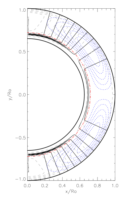
Figure 1: Isorotation lines of the solar angular velocity as inferred from helioseismology observations (continuous lines) and the adopted meridional circulation stream lines. The red dot-dashed line shows the boundary between the overshoot layer and the convection zone.

The profiles that we employ describe the results of recent helioseismology inversions or numerical simulations. For the differential rotation, we consider a profile mapped from helioseismology (see the continuous lines of Figure 1). For the meridional flow, we consider one cell per meridional quadrant, as usually assumed (doted lines in Figure 1). The alpha term ($\alpha B_{\phi}$) is concentrated between $0.95R_{\odot}$ and $R_{\odot}$ and at the latitudes where the sunspots appear (see the continuous lines in Figure 2). Since it must result the emergence of magnetic flux tubes, we assume this term to be proportional to the toroidal field $B_{\phi}(r_{c},\theta)$ at the overshoot interface between the radiative and the convective regions, $r_{c}$$=$$0.715R_{\odot}$. For the magnetic diffusion, we consider only one gradient of diffusivity located at $r_{c}$ which separates the radiative stable region (with $\eta_{rz}$$=$$10^{9}$ cm s^-2) from the convective turbulent layer (with $\eta_{cz}$$=$$10^{11}$ cm s^-2) (see the dotted line in the upper panel of Figure 2).

Figure 2: Radial and latitudinal profiles for $\alpha$ (continuous line), $\eta_{T}$ (dotted line) and for the pumping terms $\gamma_{r}$ and $\gamma_{\theta}$ (dashed and dot-dashed lines, respectively). All the profiles are normalized to their maximum value. Extracted from Guerrero & de Gouveia Dal Pino (2008).

0.3 The location of the solar dynamo

As remarked before, the differential rotation pattern which is responsible for the $\Omega$ effect, is revealed by high resolution helioseismology observations. It describes a solid-body rotation for the radiative core, and a differentially rotating convective layer with a retrograde velocity with respect to the radiative interior at higher latitudes and a pro-grade velocity at lower latitudes. The interface that bounds the solid-body rotation zone is named tachocline $-$ its exact location and width have not been established yet. Another radial shear layer has been recently identified just below the solar photosphere in the upper $35$ Mm of the sun (Corbard & Thompson, 2002) (see the gray dashed line in Fig. 1). With this newly discovered shear layer, it is even more difficult to define where the dynamo operates. There has been so far, an apparent common agreement that the dynamo is operating at the tachocline. However this possibility has several problems (Brandenburg, 2005). One of the main difficulties is that toroidal flux ropes formed in the tachocline should have intensities $\sim$ $10^{4}$-$10^{5}$ G in order to become buoyantly unstable and to emerge at the surface to form a BMR the appropriate tilt given by the Joy’s law (D’Silva & Choudhuri, 1993; Fan et al., 1993; Caligari et al., 1995, 1998; Fan & Fisher, 1996; Fan, 2004). One important limitation of this scenario is that $10^{5}$ G results an energy density that is an order of magnitude larger than the equipartition value, so that a stable layer is required to store and amplify this magnetic field. This raises another question with regard to the way in which the magnetic flux is dragged down to deeper layers. In recent work (Guerrero & de Gouveia Dal Pino, 2007a), we have explored the contributions of the shear terms in the dynamo equation, $({\bf B_{p}}\cdot\nabla)\Omega$$=$$B_{r}{\partial\Omega/\partial r}+B_{\theta}/r\partial\Omega\partial\theta$ with the aim of determining where the most strong toroidal magnetic fields are produced. We found that the radial shear component is about two orders of magnitude smaller than the latitudinal component. Therefore, when a new toroidal field begins to develop its growth is dominated by the latitudinal shear. Its amplification begins in the bulk of the convection zone and it is transported to the stable layer where it must reach the desired magnitude (see Fig. 3). How this flux is transported is the subject of the next section.

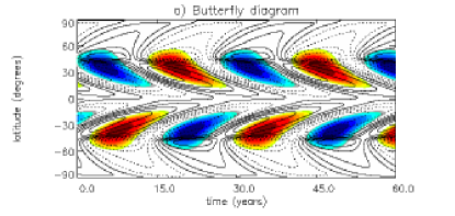
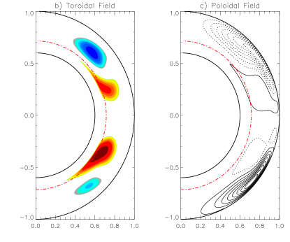
Figure 3: (a) Butterfly diagram and latitudinal snapshots for the toroidal (b) and the poloidal (c) fields. The dark (blue) and light (red) gray (color) scales represent positive and negative toroidal fields, respectively; the continuous and dashed lines represent the positive and negative poloidal fields. Only toroidal fields greater than $2\times 10^{4}$ G (the most external contours) are shown in panels (a) and (b). This model started with an anti-symmetric initial condition (see §6 for details). Extracted from Guerrero & de Gouveia Dal Pino (2008).

If a near-surface shear layer is turned on in the model (Guerrero & de Gouveia Dal Pino 2008 and references therein), two main branches appear in the butterfly diagram (Fig. 4). One is migrating poleward (at high latitudes) and another is migrating equatorward (below $45^{\circ}$). This result is expected if the Parker-Yoshimura sign rule (Parker, 1955; Yoshimura, 1975) applies. This contribution to the toroidal field was previously explored in a Babcock-Leighton dynamo by Dikpati et al. (2002). They have discarded the near-surface radial shear layer because it generates butterfly diagrams in which a positive toroidal field gives rise to a negative radial field, which is exactly the opposite to the observed. Our results, on the other hand, present the correct phase lag between the fields. This difference probably arises from the fact that we are using a lower meridional circulation amplitude. Anyway, as can be seen in Fig. 4, the polar branches are strong enough to generate also undesirable sunspots close to the poles. The period increases to $15.6$ y due to the fact that the dominant dynamo action at the surface goes in the opposite direction to the meridional flow (i.e, the dynamo wave direction is dominating over the meridional flow).

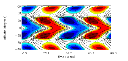
Figure 4: Butterfly diagram for a model with the same parameters as in Fig. 3, but with near-surface shear layer. For this model $T$$=$$15.6$ yr $B_{\phi_{max}}(r$$=$$0.715)$$=$$1.1\times 10^{5}$, $B_{\phi_{max}}(r$$=$$0.98)$$=$$1.9\times 10^{4}$ G and $B_{r_{max}}$$=$$131.7$ G. This model started with symmetric initial conditions. Extracted from Guerrero & de Gouveia Dal Pino (2008).

0.4 Flux transport mechanisms

For an $\alpha\Omega$ dynamo, the Parker-Yoshimura sign rule (Parker, 1955; Yoshimura, 1975) establishes that the direction of the dynamo wave is equatorward or poleward if the product $\alpha$ $\cdot$ ${\partial\Omega/\partial r}$ is $<$ or $>$$0$, respectively. Hence, models with a solar like rotation law operating at the tachocline, with a positive $\alpha$ effect in the northern hemisphere, as believed, and without meridional circulation, should result a solution with magnetic branches migrating in the opposite way to that observed (Küker et al., 2001). Models with one cell of meridional circulation, poleward at the surface and equatorward at the base of the convection zone, produce results with the appropriate direction of propagation (Dikpati & Charbonneau, 1999; Küker et al., 2001; Bonanno et al., 2002). It was demonstrated also that the meridional circulation sets the period of the cycle (Dikpati & Charbonneau, 1999) and that it is the most logical way to transport the novel poloidal fields to the inner layers in the dynamo process. These models in which the time of the cycle fits better with the advective time than with the diffusive one are usually called advection dominated or flux-transport dynamos. There is, however, an important problem with these models: they require a large scale meridional flow and this is observed only at the surface. It is possible that the real meridional flow is too weak at the inner regions to penetrate the overshoot layer and the tachocline (Gilman & Miesch, 2004; Rüdiger et al., 2005), or perhaps, it has a multicell pattern (Mitra-Kraev & Thompson, 2007; Bonanno et al., 2006; Jouve & Brun, 2007). If this is the case, it is very hard to explain the equatorward migration of the toroidal branches and it is necessary to find another flux-transport mechanism. The turbulent pumping seems to be a good candidate.

The turbulent pumping effect corresponds to the transport, in all directions, of magnetic flux due to the presence of density (buoyancy) and turbulence (diamagnetism) gradients in convectively unstable layers. In the FOSA (First Order Smoothing Approximation, see e.g. Brandenburg & Subramanian, 2005b, and references therein), the radial component of the diamagnetic pumping can be calculated assuming a linear dependence with the variations in the magnetic diffusivity $U_{dia}$$=$$-\nabla\eta_{T}/2$; the buoyancy component depends on the density gradients $U_{buo}$$=$$-\eta\nabla\rho/\rho$. In the boundary between the solar convection zone and the overshoot layer, it is probable that the diamagnetic velocity is of the order of $50$ ms^-1 (Kitchatinov & Rüdiger, 2008). This value strengthens the importance of the pumping relative to the assumed radial meridional flow velocity which is $<10$ ms^-1. For our model, we obtain $U_{dia}$$=$$\simeq$$47$ cm s^-1 when a variation of two orders of magnitude is considered in the diffusivity in a thin region of $0.015R_{\odot}$ (Guerrero & de Gouveia Dal Pino, 2008) (the buoyancy component of the pumping is not considered because the density is not a parameter in kinematic models).

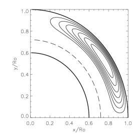
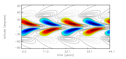
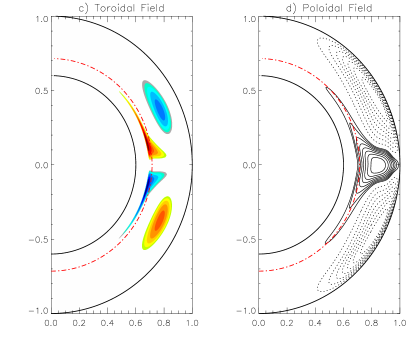
Figure 5: Meridional flow streamlines and the butterfly diagram for a model with the full pumping term, but with a shallow meridional flow penetration with a depth of only $0.8R_{\odot}$, $U_{0}$$=$$1300$ cm s^-1, $\gamma_{\theta 0}$$=$$90$ cm s^-1 and $\gamma_{r0}$$=$$30$ cm s^-1. For this model we obtain $T$$=$$10.8$ yr, $B_{\phi_{max}}$$=$$4.5\times 10^{4}$ G and $B_{r_{max}}$$=$$154.9$ G. This model started with anti-symmetric initial conditions. Extracted from Guerrero & de Gouveia Dal Pino (2008).

The effects of turbulent pumping have been rarely considered in mean field dynamo models. A first approach showing its importance in the solar cycle was made by Brandenburg et al. (1992); since then few works have incorporated the diamagnetic pumping component in the dynamo equation as an extra diffusive term that can provide a downward velocity, as discussed above (Küker et al., 2001; Bonanno et al., 2002, 2006). More recently, Käpylä et al. (2006b) have implemented simulations of the mean field dynamo in the distributed regime, including all the dynamo coefficients previously evaluated in magneto-convection simulations (Ossendrijver et al., 2002; Käpylä et al., 2006a). They produced butterfly diagrams that resemble the observations. However, to our knowledge no special efforts have been made to study the pumping effects in the meridional plane (i.e., inside the convection zone) or in a BL description.

We have included the turbulent pumping terms (see the dashed and dot-dashed lines in Fig. 2 which correspond to the radial, $\gamma_{r}$, and latitudinal, $\gamma_{\theta}$, pumping terms) calculated from local magneto-convection simulations (Ossendrijver et al., 2002; Käpylä et al., 2006a) into the induction equation (eq. 1).

For a dynamo model operating at the tachocline, we find that the pumping terms lead to a distinct latitudinal distribution of the toroidal fields when compared with the results of Fig. 3. The turbulent and density gradient levels present in the convectively unstable layer cause the pumping of the magnetic field both down and equartorward, allowing its amplification within the stable layer and its later emergence at latitudes very near the equator.

If we also include in this model recent helioseismic results (Mitra-Kraev & Thompson, 2007) that suggest that the return point of the meridional circulation can be at $\sim 0.95R_{\odot}$, at lower regions, beneath $\sim 0.8R_{\odot}$, a second weaker convection cell or even a null large scale meridional flow can exist. In Figure 5, we obtain a butterfly diagram that agrees with the main features of the solar cycle, besides, we find that in this case, it is the pumping terms that regulate the period of the cycle, leading to a $different$ $class$ of dynamo that is advection-dominated by turbulent pumping rather than by a deep meridional flow.

For the dynamo model operating at the near-surface shear layer, we find that the toroidal fields created at high latitudes are efficiently pushed down before reaching a significant amplitude, so that only the equatorial branches below $45^{\circ}$ survive (see Fig. 6). This result is explained by the fact that the radial pumping component has its maximum amplitude close to the poles (see the dashed line in Fig. 2). These results also agree with the observations.

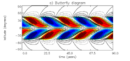
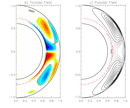
Figure 6: The same as in Fig. 5, but for a model with near-surface shear action. For this model $T$$=$$16.3$ yr $B_{\phi_{max}}(r$$=$$0.715)$$=$$9.7\times 10^{4}$, $B_{\phi_{max}}(r$$=$$0.98)$$=$$1.9\times 10^{4}$ G and $B_{r_{max}}$$=$$164.4$ G. This model started with symmetric initial conditions. Extracted from Guerrero & de Gouveia Dal Pino (2008).

0.5 How to explain the observed latitudes of the solar activity?

The radial shear at the tachocline has its maximum amplitude in regions close to the poles, for this reason, it is a common problem in mean field dynamo models to present large undesirable toroidal magnetic fields in the polar regions. Nandy & Choudhuri (2002) proposed a deep meridional flow as a way to avoid the formation of strong toroidal fields at high latitudes. Under this assumption, the strong toroidal magnetic fields formed at high latitudes are pushed down, inside the radiative zone, by the meridional flow and are stored there until they reach latitudes below $30^{\circ}$. However this assumption may lead to undesirable mixing of the chemical elements between the radiative and convective zones and to problems regarding the angular momentum transfer. Besides, some results of numerical simulations show that the meridional flow is unable to penetrate the tachocline (Gilman & Miesch, 2004; Rüdiger et al., 2005).

We have explored this subject in two ways. First, we built a hybrid model in which we combined the profiles used by Nandy & Choudhuri (2002) with those used by Dikpati & Charbonneau (1999) and allowed a deep meridional flow (Guerrero & Muñoz, 2004). We found that the high-latitude toroidal field is sensitive to the model. Then, we explored this problem by changing the shape and the thickness of the solar tachocline (Guerrero & de Gouveia Dal Pino, 2007a, b) and have found that the thinner the tachocline, the smaller the intensity of the toroidal magnetic field at high latitudes (see Fig. 7). A thin tachocline must be fully contained inside the overshoot zone, in such a way that only part of the poloidal magnetic field is able to reach it and then produce a small quantity of toroidal field. The toroidal field generated there is not strong enough to emerge. In Fig. 8, we compare the toroidal fields produced for a thin tachocline with those produced with an intermediate one. This result is also dependent of the magnetic diffusivity in the convection zone, as it can be seen in Fig. 7, however, for a thin tachocline the models always result weak toroidal fields above $60^{\circ}$.

Figure 7: Maximum of the toroidal magnetic field at the top of the tacholine as a function of the diffusivity (in log-scale) at a latitude of $60^{\circ}$. The different line styles represent different widths of the tachocline $d_{1}$. The dotted line represents the limit between buoyant and non-buoyant magnetic fields $5\times 10^{4}$ G. Only the values below this line will appear at the desired latitudes Extracted from Guerrero & de Gouveia Dal Pino (2007a).

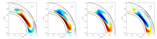
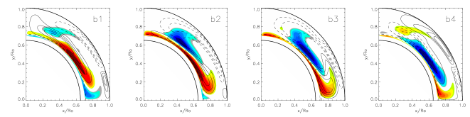
Figure 8: Snapshots of the positive (negative) toroidal field contours are shown in blue (red) scale together with the field lines of the positive (negative) poloidal field in continuous (dashed) lines, for four different times ($T/8$, $T/4$, $3T/8$ and $T/2$) along a half 11-year cycle. The upper (a) and middle (b) panels present the same snapshots for models with a thin ($0.02R_{\odot}$) and an intermediate ($0.06R_{\odot}$) tachocline Extracted from Guerrero & de Gouveia Dal Pino (2007b).

With regard to this question of the distribution of the toroidal field, the role of the pumping is also important. While it pushes poloidal fields inside the tachocline, it also pumps all the field equatorward, in such a way that the toroidal fields formed inside the convection zone due to latitudinal shear will go fast to the stable region where they are stored and amplified before the eruption (Guerrero & de Gouveia Dal Pino, 2008).

In the case that we consider the sunspots as the product of toroidal fields being formed at the near-surface layer, the latitude of activity is easily explained by the pumping, as described in the previous section (see Fig. 6).

0.6 The parity problem

The anti-symmetric parity observed in the solar cycle is one of the most challenging questions in the solar dynamo theory. The magnetic parity in a model may depend on the location of the $\alpha$ effect (Dikpati & Gilman, 2001; Bonanno et al., 2002), or on the diffusive coupling between the poloidal field in both hemispheres (Chatterjee et al., 2004), but it may also be the result of the imprint of the quadrupolar form of the meridional flow on the poloidal magnetic field, as argued by Charbonneau (2007). This could explain why models with the $\alpha$ effect located at the upper layers (where the magnetic Reynols number and the quadrupolar imprint of the meridional flow are larger) tend to a quadrupolar parity faster than models with the $\alpha$ effect located at the tachocline.

We have explored a little this problem in order to see whether the turbulent pumping plays some role in it. We have found that models without pumping result a quadrupolar solution. When beginning with a dipolar initial condition, they spend several thousand years before switching to a quadrupolar solution (see Fig. 9a). This result diverges from the one obtained by Dikpati & Gilman (2001) or Chatterjee et al. (2004) in which the change begins only after around $500$ yr. This result indicates the strong sensitivity of the parity to the initial conditions, in such a way that, for example, the present parity observed in the sun could be temporary.

The models with full pumping (e.g., Fig. 5) conserve the initial parity either it is symmetric or anti-symmetric (see Fig 9b). This suggests that the strong quadrupolar imprint due to meridional circulation can be washed out when the full turbulent pumping is switched on.

On the other hand, the full pumping in models that include near-surface shear tend to the dipolar parity from the first years of integration (see continuous line of Fig. 9c). We explain this result as a product of a better coupling between the poloidal fields in both hemispheres (this coupling is due to the local $\alpha$ effect considered in these cases), plus the action of the pumping eliminating the effect of the quadrupolar component of the meridional flow on the poloidal magnetic field.

Figure 9: Parity curves for the three classes of models considered, i.e., (a) for models without pumping (as, e.g., in Fig. 3); (b) for models with full pumping (as, e.g., in Fig. 5); and (c) for models with near-surface shear (as, e.g., in Figs. 4 and 6). In the panels (a) and (b), the continuous, dashed and dot-dashed lines correspond to symmetric, anti-symmetric and random initial conditions, respectively. In panel (c), the continuous line is used for the model with turbulent pumping while the dashed line is for the model without pumping Extracted from Guerrero & de Gouveia Dal Pino (2008).

0.7 Summary and discussion

We have used a mean field dynamo model in the BL approach in order to look for answers to four current problems widely reported in the literature of solar dynamo modeling.

Our results confirm the idea that there should be a magnetic layer below the convection zone where magnetic fields which are mainly produced in the convection zone are stored. We have found that it is possible to have a flux-transport dynamo without a well defined meridional flow pattern, dominated by the pumping advection. However, efforts in order to obtain a more realistic profile for the meridional velocity profile are still required, as well as to obtain a better comprehension of the real contribution of the pumping velocities.

Nevertheless, numerical simulations including near-surface shear as observed, provide also support for a near-surface magnetic layer, since toroidal fields with intensities between $10^{3}$ - $10^{4}$ G are formed there and since the radial differential rotation is negative at lower latitudes, the direction of migration of the butterfly wings constructed with these fields reproduces the one observed (e.g., Fig. 6).

The latitude of activity established by the observations (between $\pm 30^{\circ}$) can be explained by both scenarios above for the magnetic layer. For magnetic fields being stored in the overshoot region, a thin ($\lesssim 0.2R_{\odot}$) tachocline could be the solution to avoid strong toroidal fields at the polar regions. On the other hand, if the near-surface shear is considered, then the magnetic pumping provides the required downwards flux of the weak polar fields, letting only the toroidal fields to survive at the active latitudes.

The parity in a dynamo solution is a problem that requires especial attention. We have investigated this problem looking for the role that the pumping could play in the solutions. Our simulations support the idea that the quadrupolar solution in most of the models is due to the strong quadrupolar imprint due to the one-cell meridional flow pattern. This imprint is larger at the surface than at the bottom of the convection zone, therefore the results of Dikpati & Gilman (2001); Bonanno et al. (2002) which suggest that an $\alpha$ effect operating at the tachocline results an anti-symmetric solution, could be explained by this fact. We suggest that models with an $\alpha$ effect operating close to the surface are also able to generate anti-symmetric solutions, as observed, if a mechanism such as pumping cleans the quadrupolar imprint.

More observational and theoretical efforts are necessary in order to determine where the feet of the magnetic flux tubes responsible for the sunspots are located. This is an issue that needs to be solved before a more realistic coherent dynamo model can be constructed.

References

- Babcock (1961) Babcock, H. W. 1961, ApJ, 133, 572
- Bonanno et al. (2006) Bonanno, A., Elstner, D., & Belvedere, G. 2006, Astronomische Nachrichten, 327, 680
- Bonanno et al. (2002) Bonanno, A., Elstner, D., Rüdiger, G., & Belvedere, G. 2002, A&A, 390, 673
- Brandenburg (2005) Brandenburg, A. 2005, ApJ, 625, 539
- Brandenburg et al. (1992) Brandenburg, A., Moss, D., & Tuominen, I. 1992, in Astronomical Society of the Pacific Conference Series, Vol. 27, The Solar Cycle, ed. K. L. Harvey, 536–+
- Brandenburg & Subramanian (2005a) Brandenburg, A. & Subramanian, K. 2005a, Phys. Rep., 417, 1
- Brandenburg & Subramanian (2005b) —. 2005b, Phys. Rep., 417, 1
- Brun et al. (2004) Brun, A. S., Miesch, M. S., & Toomre, J. 2004, ApJ, 614, 1073
- Caligari et al. (1995) Caligari, P., Moreno-Insertis, F., & Schussler, M. 1995, ApJ, 441, 886
- Caligari et al. (1998) —. 1998, ApJ, 502, 481
- Cattaneo & Hughes (1996) Cattaneo, F. & Hughes, D. W. 1996, Phys. Rev. E, 54, 4532
- Charbonneau (2007) Charbonneau, P. 2007, Advances in Space Research, 39, 1661
- Chatterjee et al. (2004) Chatterjee, P., Nandy, D., & Choudhuri, A. R. 2004, A&A, 427, 1019
- Corbard & Thompson (2002) Corbard, T. & Thompson, M. J. 2002, Sol. Phys., 205, 211
- Dikpati & Charbonneau (1999) Dikpati, M. & Charbonneau, P. 1999, ApJ, 518, 508
- Dikpati et al. (2002) Dikpati, M., Corbard, T., Thompson, M. J., & Gilman, P. A. 2002, ApJ, 575, L41
- Dikpati & Gilman (2001) Dikpati, M. & Gilman, P. A. 2001, ApJ, 559, 428
- D’Silva & Choudhuri (1993) D’Silva, S. & Choudhuri, A. R. 1993, A&A, 272, 621
- Fan (2004) Fan, Y. 2004, Living Rev. Solar Phys., 1, 1
- Fan & Fisher (1996) Fan, Y. & Fisher, G. H. 1996, Sol. Phys., 166, 17
- Fan et al. (1993) Fan, Y., Fisher, G. H., & Deluca, E. E. 1993, ApJ, 405, 390
- Gilman & Miesch (2004) Gilman, P. A. & Miesch, M. S. 2004, ApJ, 611, 568
- Guerrero & de Gouveia Dal Pino (2007a) Guerrero, G. & de Gouveia Dal Pino, E. M. 2007a, A&A, 464, 341
- Guerrero & de Gouveia Dal Pino (2008) —. 2008, A&A, 485, 267
- Guerrero & de Gouveia Dal Pino (2007b) Guerrero, G. A. & de Gouveia Dal Pino, E. M. 2007b, Astronomische Nachrichten, 328, 1122
- Guerrero & Muñoz (2004) Guerrero, G. A. & Muñoz, J. D. 2004, MNRAS, 350, 317
- Jouve & Brun (2007) Jouve, L. & Brun, A. S. 2007, A&A, 474, 239
- Käpylä et al. (2006a) Käpylä, P. J., Korpi, M. J., Ossendrijver, M., & Stix, M. 2006a, A&A, 455, 401
- Käpylä et al. (2006b) Käpylä, P. J., Korpi, M. J., & Tuominen, I. 2006b, Astronomische Nachrichten, 327, 884
- Kitchatinov & Rüdiger (2008) Kitchatinov, L. L. & Rüdiger, G. 2008, Astronomische Nachrichten, 329, 372
- Küker et al. (2001) Küker, M., Rüdiger, G., & Schultz, M. 2001, A&A, 374, 301
- Leighton (1969) Leighton, R. B. 1969, ApJ, 156, 1
- Mitra-Kraev & Thompson (2007) Mitra-Kraev, U. & Thompson, M. J. 2007, ArXiv e-prints, 711
- Nandy & Choudhuri (2002) Nandy, D. & Choudhuri, A. R. 2002, Science, 296, 1671
- Ossendrijver et al. (2002) Ossendrijver, M., Stix, M., Brandenburg, A., & Rüdiger, G. 2002, A&A, 394, 735
- Parker (1955) Parker, E. N. 1955, ApJ, 122, 293
- Rüdiger et al. (2005) Rüdiger, G., Kitchatinov, L. L., & Arlt, R. 2005, A&A, 444, L53
- Schwabe (1844) Schwabe, M. 1844, Astronomische Nachrichten, 21, 233
- Vainshtein & Cattaneo (1992) Vainshtein, S. I. & Cattaneo, F. 1992, ApJ, 393, 165
- Vishniac & Cho (2001) Vishniac, E. T. & Cho, J. 2001, ApJ, 550, 752
- Wang et al. (1989) Wang, Y.-M., Nash, A. G., & Sheeley, Jr., N. R. 1989, Science, 245, 712
- Wang et al. (1991) Wang, Y.-M., Sheeley, Jr., N. R., & Nash, A. G. 1991, ApJ, 383, 431
- Yoshimura (1975) Yoshimura, H. 1975, ApJ, 201, 740