Multiple temperature scales of the periodic Anderson model:
the slave bosons approach

Abstract

The thermodynamic and transport properties of intermetallic compounds with Ce, Eu, and Yb ions are discussed using the periodic Anderson model with an infinite correlation between $f$ electrons. At high temperatures, these systems exhibit typical features that can be understood in terms of a single impurity Anderson or Kondo model with Kondo scale T_K. At low temperatures, the normal state is governed by the Fermi liquid (FL) laws with characteristic energy scale T${}_{0}.$ The slave boson solution of the periodic model shows that T₀ and T_K depend not only on the degeneracy and the splitting of the $f$ states, the number of $c$ and $f$ electrons, and their coupling, but also on the shape of the conduction electrons density of states ($c$ DOS) in the vicinity of the chemical potential.

We show that the details of the band structure determine the ratio T₀/T_K and that the crossover between the high- and low-temperature regimes in ordered compounds is system-dependent. A sharp peak in the $c$ DOS yields T${}_{0}\ll$T_K and explains the ’slow crossover’ observed in YbAl₃ or YbMgCu₄. A minimum in the $c$ DOS yields T${}_{0}\gg$T_K, which leads to the abrupt transition between the high- and low-temperature regimes in YbInCu₄. In the case of CeCu₂Ge₂ and CeCu₂Si₂, where T${}_{0}\simeq T_{K}$, the slave boson solution explains the pressure experiments which reveal sharp peaks in the T² coefficient of the electrical resistance, $A=\rho(T)/T^{2}$, and the residual resistance. These peaks are due to the change in the degeneracy of the $f$ states induced by the applied pressure.

The FL laws explain also the correlation between the specific heat coefficient $\gamma=C_{V}/T$ and the slope of the thermopower $\alpha(T)/T$, or between $\gamma$ and the $A$ coefficient of the resistivity. For $N$-fold degenerate model, the FL laws explain the deviations from universal value of the Kadowaki-Woods ratio, $R_{KW}=A/\gamma^{2}$, and the ratio $q=lim_{\{T\to 0\}}\alpha/\gamma T$. The renormalization of transport coefficients can invalidate the Wiedemann-Franz law and lead to an enhancement of the thermoelectric figure-of-merit. We show that the low-temperature response of the periodic Anderson model can be enhanced (or reduced) with respect to the predictions based on the single-impurity models that give the same high-temperature behavior.

I Introduction

Intermetallic compounds containing Cerium, Ytterbium and Europium ions exhibit a number of remarkable phenomena, like the heavy fermion mass enhancement, valence fluctuations, huge thermopower, spin-charge separation, unconventional magnetism and superconductivity, etc. These systems have been studied for several decades and are still attracting considerable attention. The initial focus was on dilute alloys with magnetic 3$d$ and 4$f$ impurities, where the low- and high-temperature behavior is qualitatively different. At high temperatures, the experimental data indicate that the $f$ states are localized and weakly coupled to conduction states. The susceptibility is of the Curie-Weiss form and entropy is large, as expected of nearly free $f$ ions. At the same time, the logarithmic resistivity and large thermopower are typical of the conduction ($c$) electrons weakly perturbed by the local moments. Such a behavior is explained by the perturbative solution of the Anderson or Kondo models, which yield the low-energy correlation functions as universal functions of reduced temperature T/T_K, where T_K is the Kondo temperature. At low temperatures, the experimental data show that the susceptibility is Pauli like, the specific heat and entropy are linear in temperature, and transport coefficients are given by simple powers of reduced temperature T/T_K. Close to the ground state, the $c$ and $f$ states seem to form a non-magnetic singlet with the fermionic excitation spectrum and energy scale T_K. The overall behavior of dilute alloys with paramagnetic impurities is nearly the same when plotted on the $T/T_{K}$ scale, even though the values of T_K vary by orders of magnitude. Unlike the high-temperature data, neither the crossover nor the low-temperature behavior can be understood in terms of the perturbation theory which treats the conduction electrons and the local moments as separate entities. The fact that the low-temperature scale coincides with the high-temperature one and that the crossover from the weak to the strong coupling regime takes place around T_K are the most prominent features of dilute Kondo systems.

The dilute alloy problem has been explained after several decades of intensive work by the exact solutions of the Kondo and the Anderson models. Early calculations considered the models in which the conduction electrons with a constant density of states ($c$ DOS) are exchange scattered on a spin-1/2 local moment. The solution was obtained by the variety of methods, like the perturbative scalingAnderson (1970), the numerical renormalization groupWilson (1975), the Fermi liquid theoryNozières (1974); Yamada (1975), and Bethe AnsatzTsvelick and Wiegmann (1983). These results reveal that the effective coupling between the free fermions and degenerate local moments increases at low temperatures and diverges in the ground state, which explains the breakdown of the perturbation theory. However, the simple models cannot provide a quantitative description of dilute Kondo alloys; a realistic modeling has to take into account the details of the local states and the band structure of the host, and consider additional scattering mechanisms. In Kondo systems with Ce and Yb ions, the splitting of the 4$f$ states by the spin-orbit and the crystal field (CF) effects can change the effective degeneracy of the system, reduce the Kondo scale, and lead to the seemingly complicated features, like the multiple peaks in the resistivity or the sign change of the thermopower and the Hall effect. A non-constant $c$ DOS leads also to a complicated low-temperature behavior. For example, Whithoff and Fradkin Withoff and Fradkin (1990) have found that the $c$ DOS with a power-law singularity leads to a critical coupling $J_{c}$ that separates different ground states. For $J>J_{c}$, the ground state is of the strong coupling type, while for $J<J_{c}$ the renormalized coupling decreases with temperature and the “usual” Kondo screening of local moments does not occurVojta and Bulla (2002). Nevertheless, despite a conduction electron pseudo-gap, it has been shown that Kondo-lattice screening can be more stable than in the single Kondo impurity case Sheehy and Schmalian (2008).

The Kondo problem becomes much more difficult for stoichiometric compounds in which a magnetic ion is present in each unit cell. The high-temperature features can still be explained by an effective single-impurity model, if one takes into account additional splittings of the $f$ states and/or the fact that $c$ DOS can change rapidly in the vicinity of the chemical potential. The perturbation theory provides a consistent picture of the high-temperature data: it yields the correct Kondo scale, explains the Curie-Weiss behavior of the susceptibility and the logarithmic decrease of the resistivity and thermopower, and accounts for the well resolved CF excitations seen in neutron experiments. However, at sufficiently low temperatures the scattering becomes coherent and one finds new features that cannot be explained by the single impurity models. The onset of coherence is most clearly seen in the electrical resistivity which drops to very small values, and in the optical conductivity which shows the development of a low-frequency Drude peak and a small hybridization gap close to the chemical potential. At lowest temperatures, the Fermi liquid laws often emerge: the resistivity is quadratic and the thermopower a linear function of temperature; the specific heat and the magnetic susceptibility are much enhanced, indicating a large effective electronic mass; the de Haas-van Alphen experiments show that $f$ electrons contribute to the Fermi volume. The low-temperature ratios of various correlation functions, like the Wilson ratio, $\chi/\gamma$ or the Kadowaki-Woods ratio, $A/\gamma^{2}$, assume the universal values. Here, $\gamma$ and $\chi$, denote the $T\to 0$ limit of the specific heat coefficient and the magnetic susceptibility, and $A$ is the coefficient of the $T^{2}$ term in the resistivity. The universality of these ratios indicates that the ground state properties depend on a single energy scale T₀. However, unlike in dilute alloys, this FL scale T₀ can be much different from T_K.

In this paper we study the periodic systems with 4$f$ ions and show that the relative magnitude of the Kondo and the FL scale depends on the shape of the unperturbed conduction states. The Anderson lattice with an enhanced DOS around the chemical potential has T${}_{0}\ll$T_K, which explains the gradual transition between the coherent and the incoherent regimes (slow crossover) observed in YbAl₃ Bauer et al. (2004). A pseudo-gap or a reduced $c$ DOS close to the chemical potential yields T${}_{K}\ll$T₀, which explains the abrupt valence-change transition observed in Yb- and Eu-based intermetallic compounds, like YbInCu₄ Sarrao (1999), EuNi₂(Si_1-xGe_x)₂ Wada et al. (1997) or Eu(Pd_1-xPt_x)₂Si₂ Mitsuda et al. (2000). In the case of CeCu₂Ge₂ and CeCu₂Si₂, where T_K and T₀ seem to be of the same order of magnitude, we show that the pressure-dependence of the $A(P)$ coefficient and the residual resistance is driven by the change in the degeneracy of the $f$ states.

The paper is organized as follows. Section  II explains briefly the slave boson formalism for the Anderson model and defines its low- and high-temperature scales T₀ and T_K. This section provides also the relationship between the $c$ DOS and the relative magnitude of T₀ and T_K, discusses the effects of the magnetic field, and shows how to express the transport coefficients in terms of T/T₀. In Section  III we discuss the relevance of these results for the experimental data on various intermetallic compounds in which the ratio T${}_{0}/$T_K can be much smaller or larger than one. For the case T${}_{0}\simeq$T_K, we discuss the pressure anomalies in the $A$ coefficient and the residual resistance induced by the changes in the effective degeneracy of the $f$ states.

II Slave boson solution of the periodic Anderson model

II.1 The mean-field self consistent equations in the limit $U\to\infty$

The periodic Anderson Model (PAM) Hamiltonian is written in the limit of an infinite correlation between $f$ electrons, $U=+\infty$, as

$$H= \sum_{{\bf k}\sigma}\epsilon_{\bf k}c_{{\bf k}\sigma}^{\dagger}c_{{\bf k}\sigma}+E_{f}\sum_{i\sigma}f_{i\sigma}^{\dagger}f_{i\sigma}+V\sum_{i\sigma}[c_{i\sigma}^{\dagger}f_{i\sigma}+f_{i\sigma}^{\dagger}c_{i\sigma}]-\mu\sum_{i\sigma}[f_{i\sigma}^{\dagger}f_{i\sigma}+c_{i\sigma}^{\dagger}c_{i\sigma}]$$ (1)

$$+ h\sum_{i}\left[g_{c}(c_{i\uparrow}^{\dagger}c_{i\uparrow}-c_{i\downarrow}^{\dagger}c_{i\downarrow})+g_{f}(f_{i\uparrow}^{\dagger}f_{i\uparrow}-f_{i\downarrow}^{\dagger}f_{i\downarrow})\right]~{},$$ (2)

where $c_{i\sigma}$ and $f_{i\sigma}$ are annihilation operators for $c$ and $f$ electrons, $i$ is the site index, $\sigma=\uparrow,\downarrow$ is the spin component. $h$ is an external magnetic field, and $g_{c}$ and $g_{f}$ the Landé factors for $c$ and $f$ orbitals, respectively. The $c$ orbital describes the conduction band with energy levels $\epsilon_{\bf k}$, where ${\bf k}$ is the momentum component in the reciprocal space, the localized $f$ orbitals are characterized by energy level $E_{f}$ and the local hybridization between the two orbitals is specified by the matrix element $V$. The infinite Coulomb repulsion restricts the occupation of the $f$ states to $n_{f}\leq 1$ and we use the chemical potential $\mu$ to fix the total electronic occupation per site to $n=n_{c}+n_{f}$. The unperturbed $c$ DOS is $\rho_{0}(\omega)={1}/{\cal N}\sum_{\bf k}\delta(\omega-\epsilon_{\bf k})$, where ${\cal N}$ is the number of lattice sites. In the following, $\rho_{0}$ will be characterized by a half bandwidth $D$. Typical band-shapes and fillings considered in this work are shown in Fig. 1. All the energies (except the excitation energies) are measured with respect to the center of the $c$-band (see Fig. 1). The effective degeneracy of the model is determined by the lowest spin-orbit state or the additional crystal field splitting of the $f$ states of the Ce and Yb ions. This degeneracy can be changed by temperature, pressure or chemical pressure. Here, we consider an effective spin-1/2 model.

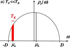
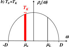
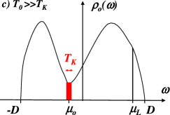
Figure 1: (Color online) Schematic plot of the non-interacting $c$ DOS $\rho_{0}(\omega)$. (a) For a regular $c$ DOS and far from the electronic half-filling we find T${}_{0}\ll$T_K. Close to the half-filling, T${}_{0}/$T_K depends on the shape of the $c$ DOS around the renormalized chemical potential $\mu$: (b) $\rho_{0}(\omega)$ is nearly constant for $\omega\sim\mu$ and T${}_{0}\sim$T_K. (c) $\mu$ is close to a minimum of $\rho_{0}(\omega)$ and T${}_{0}\gg$T_K. Here, $\mu_{0}\approx\mu$ is the chemical potential of $n_{c}=n-1$ non-interacting $c$ electrons (“small Fermi surface”), and $\mu_{L}$ is the chemical potential of $n_{c}=n$ non-interacting $c$ electrons (“large Fermi surface”).

The model defined by Eq.(2) is solved for an arbitrary $c$ DOS by the slave boson mean-field (MF) approximation Barnes (1976); Coleman (1984), which represents the $f$ states by the product of spinless bosons, $b_{i}^{\dagger}$, and auxiliary fermions of spin $\sigma=\uparrow,\downarrow$, $d_{i\sigma}^{\dagger}$. By definition, these auxiliary particle operators create the local $f$ states with no electron and one $\sigma$-spin electron, respectively; $\left|0\right>_{i}^{f}\longrightarrow b_{i}^{\dagger}\left|0\right>_{i}$ and $\left|\sigma\right>_{i}^{f}\longrightarrow d_{i\sigma}^{\dagger}\left|0\right>_{i}$. The electronic operators are related to the auxiliary operators as $f_{i\sigma}=b_{i}^{\dagger}d_{i\sigma}$, which leads to the local identities $f_{i\sigma}^{\dagger}f_{i\sigma}=d_{i\sigma}^{\dagger}d_{i\sigma}$. The doubly occupied state $\left|\uparrow\downarrow\right>_{i}^{f}$ is forbidden in the limit $U\to\infty$. The anti-commutation relations for $f$ operators as well as the physical Hilbert space are recovered by enforcing the local constraints $b_{i}^{\dagger}b_{i}+\sum_{\sigma}d_{i\sigma}^{\dagger}d_{i\sigma}=1$. The latter are satisfied by introducing the time-dependent Lagrange multipliers $\lambda_{i}(\tau)$. Assuming $g_{c}<<g_{f}$ we set $g_{c}=0$ and $g_{f}=1$, replace $hg_{f}\rightarrow h$, and rewrite the PAM Hamiltonian (2) in terms of auxiliary fermionic and bosonic operators,

$$H_{SB} = \sum_{{\bf k}\sigma}\epsilon_{\bf k}c_{{\bf k}\sigma}^{\dagger}c_{{\bf k}\sigma}+V\sum_{i\sigma}[b_{i}^{\dagger}c_{i\sigma}^{\dagger}d_{i\sigma}+b_{i}d_{i\sigma}^{\dagger}c_{i\sigma}]-\mu\sum_{i\sigma}c_{i\sigma}^{\dagger}c_{i\sigma}+h\sum_{i}(d_{i\uparrow}^{\dagger}d_{i\uparrow}-d_{i\downarrow}^{\dagger}d_{i\downarrow})$$ (3)

$$+(E_{f}-\mu)\sum_{i}(1-b_{i}^{\dagger}b_{i})+\sum_{i}\lambda_{i}\left[{b_{i}^{\dagger}b_{i}-1+\sum_{\sigma}d_{i\sigma}^{\dagger}d_{i\sigma}}\right]~{}.$$

Since the slave boson Hamiltonian (3) is invariant under the local gauge transformation $b_{i}\to b_{i}e^{i\theta_{i}}$, $d_{i\sigma}\to d_{i\sigma}e^{i\theta_{i}}$, we choose the gauge such that the bosonic fields are real, $b_{i}=b_{i}^{\dagger}\equiv r_{i}$. Finally, we make the MF approximation, assuming that the boson fields and the Lagrange multipliers are homogeneous and spin-independent constants, $r_{i}\equiv r$ and $\lambda_{i}\equiv\lambda$. Within this MF approach, which is exact in the limit of a large number of spin components, the Hamiltonian (3) becomes quadratic,

$$H_{SB}^{MF}=\sum_{{\bf k}\sigma}\left[{\epsilon_{\bf k}c_{{\bf k}\sigma}^{\dagger}c_{{\bf k}\sigma}+rV\left({c_{{\bf k}\sigma}^{\dagger}d_{{\bf k}\sigma}+d_{{\bf k}\sigma}^{\dagger}c_{{\bf k}\sigma}}\right)-\mu c_{{\bf k}\sigma}^{\dagger}c_{{\bf k}\sigma}+\lambda_{\sigma}d_{{\bf k}\sigma}^{\dagger}d_{{\bf k}\sigma}+\frac{E_{f}-\lambda-\mu}{2}(1-r^{2})}\right]~{},$$ (4)

where

$$\lambda_{\uparrow} \equiv \lambda+h~{},$$ (5)

$$\lambda_{\downarrow} \equiv \lambda-h~{}.$$ (6)

In the presence of the magnetic field $h$, the Lagrange multipliers are shifted by $\pm h$ but the up- and down-spin states remain decoupled. The self-consistent solution is obtained by minimizing the free energy $\beta{\cal F}(r,\lambda)\equiv-\ln Tre^{-\beta H}$ with respect to $r$ and $\lambda$. ¿From ${\partial{\cal F}(r,\lambda)}/{\partial r}=0$ and ${\partial{\cal F}(r,\lambda)}/{\partial\lambda}=0$ we obtain

$$2r(E_{f}-\lambda-\mu) = \frac{V}{\cal N}\sum_{{\bf k}\sigma}\langle c_{{\bf k}\sigma}^{\dagger}d_{{\bf k}\sigma}+d_{{\bf k}\sigma}^{\dagger}c_{{\bf k}\sigma}\rangle~{},$$ (7)

$$r^{2} = 1-\frac{1}{\cal N}\sum_{{\bf k}\sigma}\langle d_{{\bf k}\sigma}^{\dagger}d_{{\bf k}\sigma}\rangle~{},$$ (8)

where $\langle\cdots\rangle$ is the thermal average with respect to the MF Hamiltonian (4). The total electron occupation per site is

$$n=\frac{1}{\cal N}\sum_{i\sigma}\langle d_{i\sigma}^{\dagger}d_{i\sigma}+c_{i\sigma}^{\dagger}c_{i\sigma}\rangle\equiv n_{f}+n_{c}~{}.$$ (9)

Here, $n_{f}\equiv 1/{\cal N}\sum_{i\sigma}\langle f_{i\sigma}^{\dagger}f_{i\sigma}\rangle=1/{\cal N}\sum_{i\sigma}\langle d_{i\sigma}^{\dagger}d_{i\sigma}\rangle$ and $n_{c}\equiv 1/{\cal N}\sum_{i\sigma}\langle c_{i\sigma}^{\dagger}c_{i\sigma}\rangle$, are the average occupations per site for $f$ and $c$ orbitals, respectively. Using the relationship between the slave-boson amplitude and the total electronic occupation,

$$n_{f} = 1-r^{2}~{},$$ (10)

$$n_{c} = n-n_{f}~{}.$$ (11)

the self-consistency equations (7), (8), and (9) can be written for $r\neq 0$ as,

$$\frac{\lambda+\mu-E_{f}}{V^{2}} = \frac{1}{rV}\sum_{\sigma}\int_{-\infty}^{+\infty}\rho_{dc}^{\sigma}(\omega)n_{F}(\omega)d\omega~{},$$ (12)

$$n_{f} = \sum_{\sigma}\int_{-\infty}^{+\infty}\rho_{d}^{\sigma}(\omega)n_{F}(\omega)d\omega~{},$$ (13)

$$n_{c} = \sum_{\sigma}\int_{-\infty}^{+\infty}\rho_{c}^{\sigma}(\omega)n_{F}(\omega)d\omega~{},$$ (14)

where $n_{F}(\omega)\equiv 1/[1+e^{\beta\omega}]$ is the Fermi function and $\rho_{dc}^{\sigma}$, $\rho_{d}^{\sigma}$, $\rho_{c}^{\sigma}$ the spectral densities of the local single-particle Green’s functions of a given spin component. The Green’s functions are defined in the usual way as thermal averages of the (imaginary) time-ordered products of the appropriate creation and annihilation operators. For the quadratic MF Hamiltonian (4), the Green’s functions for $r\neq 0$ are easily calculated by the equations of motion, which yieldsZlatić et al. (2007)

$$\rho_{dc}^{\sigma}(\omega)\equiv-\frac{1}{\pi}{\mathrm{I}m}\ G_{dc}^{\sigma}(\omega) = \frac{rV}{\omega-\lambda_{\sigma}}\rho_{c}^{\sigma}(\omega)~{},$$ (15)

$$\rho_{d}^{\sigma}(\omega)\equiv-\frac{1}{\pi}{\mathrm{I}m}\ G_{d}^{\sigma}(\omega) = \frac{r^{2}V^{2}}{(\omega-\lambda_{\sigma})^{2}}\rho_{c}^{\sigma}(\omega)~{},$$ (16)

$$\rho_{c}^{\sigma}(\omega)\equiv-\frac{1}{\pi}{\mathrm{I}m}\ G_{c}^{\sigma}(\omega) = \rho_{0}\left({\omega+\mu-\frac{r^{2}V^{2}}{\omega-\lambda_{\sigma}}}\right)~{}.$$ (17)

In what follows we analyze the MF slave boson solution and discuss the effects of the band-structure.

II.2 The high-temperature solution

At high enough temperatures, the self consistency equations  (7) – (11), have only a trivial $r=\lambda=0$ solution, i.e., the effective MF hybridization in Eq. (4) vanishes, $rV=0$. This solution describes a system of decoupled $f$ and $c$ electrons. For $h=0$ and $E_{f}<\mu$, each lattice site is occupied by a single $f$ electron of spin $\sigma$ and there are $n_{c}=n-1$ conduction electrons (per site) with the $c$ DOS given by $\rho_{0}(\epsilon)$. The Fermi surface encloses $n_{c}=n-1$ points in the k-space, i.e., the $r=0$ state occupies a ”small” Fermi volume that includes ”light” $c$ electrons but not the $f$ states. The magnetic susceptibility is Curie-like, provided the direct effect of $h$ on the conduction electrons is neglected. (The Pauli-like susceptibility of $c$ electrons is negligible with respect to the Curie contribution of the $f$ states.) As long as the $c$ states are highly degenerate, $T\ll D$, their entropy is much smaller than the entropy of the localized $f$ states, and the overall entropy per site is approximately given by $S=\ln 2$. In the presence of a large magnetic field, the degeneracy of the $f$ states is lifted and the system acquires additional Zeeman energy.

Even though the trivial $r=\lambda=0$ solution does not provide a quantitative description of the PAM at high temperatures, it captures the essential qualitative point: it represents the whole system in terms of two well-defined but separated sub-systems. A more realistic approach would take into account the small coupling between the $c$ and $f$ electrons and treat it as a perturbation. This would reduce the average $f$ occupation to $n_{f}<1$, give the Curie-Weiss rather than the Curie susceptibility, and obtain the transport properties from the scattering of ”light” $c$ electrons on the $f$ ions. The resistivity calculated in such a way has logarithmic corrections to the high-temperature spin disorder limit. However, both the trivial slave boson solution and the perturbative one break down at sufficiently low temperatures.

Remarkably, the Kondo scale T_K defined by the high-temperature perturbation expansion agrees with the characteristic temperature at which the non-trivial solution of he slave boson equations emerges. In what follows we analyze the non-trivial solution of the self-consistent equations  (7) – (11) for the spin-1/2 model and show that it captures the main features of the experimental data on Ce, Eu and Yb intermetallic compounds at low temperatures. The generalization to an arbitrary $SU(N)$ symmetric Anderson model or the model with the CF split $f$ states, is straightforward (see Appendix).

II.3 Kondo temperature T_K

The non-trivial $r\neq 0$ solution of the slave boson equations is found below some critical temperature which defines the Kondo scale T_K of the periodic Anderson model. For a given set of parameters and total occupation $n$, the Kondo scale is obtained from the $r,\lambda\to 0$ limit of the equations  (7) – (9). This gives, for $h=0$,

$$\frac{2}{J(\mu)} = \int_{-\infty}^{+\infty}\frac{\rho_{0}(\omega+\mu)\tanh{(\omega/2T_{K})}}{\omega}d\omega~{},$$ (18)

$$n_{f} = 2\int_{-\infty}^{+\infty}d\omega~{}\delta(\omega-\lambda)~{}n_{F}(\omega)~{}=~{}1~{},$$ (19)

$$n_{c} = n-1=2\int_{-\infty}^{+\infty}d\omega~{}{\rho_{0}(\omega+\mu)}~{}n_{F}(\omega)~{},$$ (20)

where we introduced the Kondo coupling constant,

$$J(\mu)\equiv\frac{2V^{2}}{\mu-E_{f}}.$$ (21)

Assuming that T_K vanishes continuously and taking the limit $T_{K}\to 0$ yields the critical coupling

$$\frac{2}{J_{c}}=\int_{-\infty}^{+\infty}d\omega\frac{\rho_{0}(\omega+\mu)}{|\omega|}.$$ (22)

For a regular DOS, $\rho_{0}(\mu)\neq 0$, the r.h.s. of Eq.(22) diverges logarithmically, such that $J_{c}=0$ and any finite coupling leads to $T_{K}>0$. At T_K, the high-temperature $r=0$ phase with large paramagnetic entropy is destabilized by a transition to the low-entropy Fermi liquid phase. The Kondo scale given by Eq. (18) coincides with the solution of the scaling equations for the $SU(2)$ single-impurity Kondo model Withoff and Fradkin (1990).

The physical interpretation of the emergence of the non-trivial slave boson solution is made by the analogy with the single-impurity case. We assume that the high-temperature solution of the lattice describes a system of localized $f$ and $c$ electrons with small FS, and that the correction to the $r=0$ solution can be found by the perturbation theory in terms of $J(\mu)$. For $T>T_{K}$ the hybridization energy is small with respect to the entropic contribution to the free energy due to the degenerate $f$ states. Thus, the total free energy of the system, ${\cal F}=E-TS$, is minimized at high temperatures by the paramagnetic configuration in which the $f$ states are very weakly coupled to the $c$ states. For $T\leq T_{K}$, the entropic contribution is reduced below the hybridization energy and the paramagnetic configuration becomes thermodynamically unstable. At T_K, the crossover between the local moment and a local singlet state takes place.

In the case of an unperturbed $c$ DOS with a pseudo-gap at $\mu$, $\rho_{0}(\mu)=0$, equations (12) – (14) yield the solution with finite $J_{c}$ which separates two different low-temperature regimes. For $J>J_{c}$ the $r\neq 0$ solution emerges at temperature T_K which is the same as in the $\rho_{0}(\mu)\neq 0$ case. But for $J<J_{c}$ the $r=0$ solution persists down to $T=0$, such that the paramagnetic entropy is not removed by Kondo scattering. If the coupling is tuned by pressure or doping, a quantum phase transition can be induced at the critical value $J_{c}$ (or $V_{c}$). In the case of $c$ DOS with a gap $\Delta_{g}\ll D$ around the Fermi level we find $J_{c}\propto D/ln[D/\Delta_{g}]$. A pseudo-gap centered at the chemical potential $\mu$ and characterized by a single energy scale $D$ gives $J_{c}\propto D$. The power-law singularity $\rho_{0}(\omega)=R_{0}|\omega|^{\eta}$ gives $J_{c}=2\eta D/(\eta+1)$, which is the Whithoff and Fradkin result Withoff and Fradkin (1990); Vojta and Bulla (2002). (The constant $R_{0}$ follows from the normalization condition, $\int_{-D}^{D}\rho_{0}(\omega)=1$.)

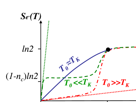
Figure 2: (Color online) Schematic plot of the electronic contribution to the entropy $S_{e^{-}}$ as a function of the normalized temperature T/T_K for three cases: T${}_{0}\gg$T_K (red dash doted line), T${}_{0}\approx$T_K (blue solid line), and $T_{0}<<T_{K}$ (green dashed line). The doted lines indicate the linear Fermi liquid regime $S_{e^{-}}(T)=T/T_{0}$, with a rescaled slope T_K/T₀. For T$>$T_K the three curves are identical, reflecting the linear contribution from the conduction band $S_{e^{-}}(T)=\ln{2}+T/D$. The black dot refers to a standard determination of T_K from the electronic entropy: $S_{e^{-}}(T_{K})=x\ln{2}$. On this schematic plot, we used $x=1$, which gives T_K as defined by the slave boson ($r=0$) solution. Experimentally, where T_K is defined by the crossover, one usually takes $x=1/2$.

To find T_K at finite $\rho_{0}(\mu)$ we use the Sommerfeld expansion of equation (18) which gives in the $T_{K}<<D$ limit the result

$$T_{K}=\alpha_{0}(D^{2}-\mu_{0}^{2})^{1/2}F_{K}e^{-1/J(\mu_{0})\rho_{0}(\mu_{0})}~{},$$ (23)

where

$$F_{K}=\exp{\left[{\int_{-(D+\mu_{0})}^{D-\mu_{0}}\frac{\rho_{0}(\mu_{0}+\omega)-\rho_{0}(\mu_{0})}{2|\omega|\rho_{0}(\mu_{0})}{d\omega}}\right]}~{}.$$ (24)

$\omega$ is measured with respect to $\mu$, $\alpha_{0}=1.13$ is a numerical constant, and $\mu_{0}$ is defined by the integral

$$\frac{n_{c}}{2}=\frac{n-1}{2}=\int_{-D}^{\mu_{0}}\rho_{0}(\omega)d\omega~{}.$$ (25)

By definition, $\mu_{0}$ is the Fermi level of $n_{c}$ non-interacting electrons which have a “small” FS. The result given by Eq. (23) is derived in Ref. Burdin et al. (2000) for a Kondo lattice with an analytic DOS. It also holds for $\rho_{0}(\omega)$ with an algebraic singularity close to $\mu_{0}$.

The Kondo temperature T_K, defined in Eq. (18) characterizes a second order phase transition. We are aware that this transition is an artefact of the slave boson MF approximation and that an exact theory would lead to a crossover instead. Experimentally, the Kondo temperature T_K is sometime estimated from the resistivity measurements, which show a maximum around T_K, or from the specific heat measurements, where T_K is identified as the temperature at which the magnetic entropy (per impurity) becomes a substantial fraction of $\ln 2$, say $S\simeq 0.5~{}\ln 2$ (see FIG. 2). Note that with this definition of T_K from the magnetic entropy we implicitly neglect the collective freezing of the entropy which is related to the Ruderman-Kittel-Kasuya-Yosida interaction.

The fact that the Anderson lattice and the single impurity Anderson model have the same Kondo scale indicates that in both cases T_K separates the paramagnetic high-entropy phase from the low-entropy phase in which the conduction electrons start forming an incoherent screening clouds which reduce the local $f$ moment in each unit cell (see FIG. 1). At temperatures at which the $c$ and $f$ states form a coherent band, and local screening clouds become correlated, the hybridization $V$ cannot be considered as a perturbation. For $T\ll T_{K}$, the Hamiltonian has to be diagonalized by non-perturbative methods and the slave boson solution provides a reasonable description of the renormalized ground state. Close to the ground state, the low-energy excitations of a periodic system are Bloch waves and we expect them to be characterized by a FL scale T₀. The question is, how is T₀ related to T_K.

II.4 The Fermi liquid scale $T_{0}$

The emergence of a strongly coupled $f-c$ fluid at T_K does not imply that Kondo scale characterizes the behavior of such a fluid close to the ground state. Electrons described by Eq. (4) form at $T=0$ a coherent Fermi liquid with an energy scale $T_{0}$, which is defined in the absence of a magnetic field as,

$$T_{0}\equiv\frac{1}{\rho^{\uparrow}(\mu)}=\frac{1}{\rho^{\downarrow}(\mu)}~{},$$ (26)

where $\rho^{\sigma}(\mu)\equiv\rho_{c}^{\sigma}(\mu)+\rho_{f}^{\sigma}(\mu)$ is the renormalized density of electronic states at the Fermi level. The scale $T_{0}$ is relevant for the $T\rightarrow 0$ properties of the periodic Anderson model; it determines the static spin susceptibility, $\chi_{loc}(T=0)\sim 1/T_{0}$, the specific heat coefficient $\gamma=C_{V}/T\sim 1/T_{0}$, and appears in the transport coefficientsZlatić et al. (2008) which are given by simple powers of reduced temperature T/T₀. The slave boson result for T₀ is computed from Eqs. (12 – 17) at $T=0$, which gives

$$\frac{E_{f}-\lambda-\mu}{2V^{2}} = \int_{-\infty}^{0}\frac{1}{\omega-\lambda}\rho_{0}\left({\omega+\mu-\frac{r^{2}V^{2}}{\omega-\lambda}}\right)d\omega~{},$$ (27)

$$\frac{n_{c}+n_{f}}{2} = \int_{-\infty}^{0}\left[1+\frac{r^{2}V^{2}}{(\omega-\lambda)^{2}}\right]\rho_{0}\left({\omega+\mu-\frac{r^{2}V^{2}}{\omega-\lambda}}\right)d\omega=\int_{-\infty}^{\mu_{L}}\rho_{0}(\omega)d\omega~{},$$ (28)

where $\rho_{0}(\omega)$ is the unperturbed $c$ DOS and $\mu_{L}$ the chemical potential of $n=n_{c}+n_{f}$ non-interacting electrons. We have

$$\mu_{L}\equiv\mu+\frac{r^{2}V^{2}}{\lambda}~{}$$ (29)

which defines the shift in the chemical potential due to the enlargement of the Fermi volume of hybridized ($r\neq 0$) system with $n$ particles with respect to the Fermi volume of the non-interacting ($r=0$) band with $n-1$ particles, $\Delta\mu\equiv\mu_{L}-\mu={r^{2}V^{2}}/{\lambda}~{}$. (This interpretation of $\Delta\mu$ neglects the width of the free-electron distribution function at temperature T_K with respect to $D$ and assumes $\mu\simeq\mu_{0}$, which holds for $n_{f}\simeq 1$.) The low-temperature FS is “enlarged” with respect to the high-temperature one, because it accommodates $n_{f}$ additional $f$ electrons. Equations  (16), (17), and (29) yield

$$\rho(\mu)=\left[1+\left(\frac{\Delta\mu}{rV}\right)^{2}\right]\rho_{0}(\mu_{L})~{},$$ (30)

which shows that $\rho(\mu)$ and T₀ depend on the shape of the unperturbed $c$ DOS and the total number of particles. In the FL regime, the entropy behaves as $T/T_{0}$, the susceptibility is constant and transport coefficients are given by simple power laws of $T/T_{0}$. The schematic phase diagram of a system with $T_{K}\neq T_{0}$ is shown schematically in Fig. 3.

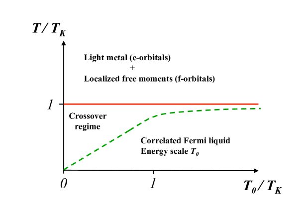
Figure 3: (Color online) Schematic phase diagram of the PAM. The reduced temperature T/T_K is plotted versus T₀/T_K, which is considered as a tunable parameter that can vary with the electronic filling, magnetic field and/or the shape of the non interacting DOS. The crossover regime can be non universal or non Fermi liquid.

The effect of the $c$ DOS can be computed analytically in the $V<<D$ limit, assuming that $\mu$ is close to $\mu_{0}$. Since $\mu_{L}$ corresponds to $n$ non-interacting electrons (”large” FS) and $\mu_{0}$ to $n_{c}\sim n-1$ electrons (”small” FS), we approximate $\Delta\mu\propto D$ (see FIG. 1). In the limit $rV/D\ll 1$, the MF Eqs. (27) and (28) give

$$\frac{E_{f}-\lambda-\mu}{2V^{2}} = {\rho_{0}(\mu)\ln{\left({\frac{r^{2}V^{2}}{(D+\mu)\Delta\mu}}\right)}-\int_{-(D+\mu)}^{\Delta\mu}\frac{\rho_{0}(\mu+\omega)-\rho_{0}(\mu)}{|\omega|}d\omega}~{},$$ (31)

$$\frac{n_{c}+n_{f}}{2} = \int_{-(D+\mu)}^{\Delta\mu}\rho_{0}(\mu+\omega)d\omega~{},$$ (32)

where we neglected the corrections of order $(rV/D)^{2}$. Solving Eqs. (31, 32) for $\lambda$ yields

$$\lambda\simeq\frac{r^{2}V^{2}}{\Delta\mu} \simeq (D+\mu_{0})~{}F_{0}~{}e^{-1/J(\mu_{0})\rho_{0}(\mu_{0})}~{},$$ (33)

where

$$F_{0}=\exp{\left[{\int_{-(D+\mu_{0})}^{\Delta\mu}\frac{\rho_{0}(\mu_{0}+\omega)-\rho_{0}(\mu_{0})}{|\omega|\rho_{0}(\mu_{0})}{d\omega}}\right]}~{}.$$ (34)

The scale T₀ of a system of particles described by the periodic Anderson model close to the ground state is obtained from equations  (26,30,33) as,

$$T_{0}=\frac{r^{2}V^{2}}{(\Delta\mu)^{2}}\frac{1}{\rho_{0}(\mu_{L})}=\frac{D+\mu_{0}}{\Delta\mu}\frac{F_{0}}{\rho_{0}(\mu_{L})}e^{-1/J(\mu_{0})\rho_{0}(\mu_{0})}~{}.$$ (35)

The scales T₀ and T_K have the same exponential dependence on the coupling constant $J(\mu_{0})$ but their pre-factors are not affected by $\rho_{0}(\omega)$ in the same way and can differ considerably. The ratio T${}_{0}/$T_K which is constant for a given set of parameters can be changed by applying pressure or magnetic field.

At temperatures low with respect to $T_{FL}={\min}\left\{T_{0},T_{K}\right\}$ the system behaves as a Fermi liquid (provided we are not too close to the Kondo insulating state) but the crossover from the high-temperature to the low-temperature regime proceeds differently for T${}_{0}\ll$T_K than for T${}_{0}\gg$T_K. This is shown schematically in Figs. 2 and  3. If T${}_{0}\ll$T_K, we have $T_{FL}=T_{0}$ and, for $T_{0}<T<T_{K}$, the system exhibits an extended non-universal behavior. If the electronic occupation $n_{c}$ is neither too small nor too close to half-filling, the MF solution of the slave boson equations Burdin et al. (2000) predicts the entropy with a plateau at about $(1-n_{c})\ln{2}$ (see FIG. 2), which characterizes $1-n_{c}$ unscreened magnetic ions. If $T_{0}\gg T_{K}$, the high-temperature perturbative regime persists all the way down to T_K, where the properties change abruptly and the system enters the FL phase characterized by T₀. Only for $T_{0}\sim T_{K}$, the lattice system is characterized by a single energy scale, as in the single impurity case.

II.5 Comparison of the Fermi liquid and the Kondo scales

The Kondo coupling $J(\mu)$ defined by Eq. (21) is always smaller than the half bandwidth $D$ of the non-interacting $c$ DOS, such that T_K and $T_{0}$ are exponentially small due to the factor $~{}\exp\{-1/J(\mu_{0})\rho_{0}(\mu_{0})\}~{}$. The analytic expressions given by Eqs. (23, 35) yield the result

$$\frac{T_{0}}{T_{K}}=\left(\frac{D+\mu_{0}}{D-\mu_{0}}\right)^{1/2}\frac{1}{\alpha_{0}\rho_{0}(\mu_{L})\Delta\mu}\frac{F_{0}}{F_{K}}~{},$$ (36)

which does not depend on the Kondo coupling $J(\mu)$ but, as discussed previously Burdin et al. (2000), varies with the electronic occupation and with the shape of the non-interacting $c$ DOS. Electronic filling effects have been discussed using the MF analysis of the Kondo lattice Burdin et al. (2000) and the DMFT solution of the periodic Anderson modelTahvildar-Zadeh et al. (1997). In the limit $n_{c}\to 0$ ($n\approx 1$), the first factor $D+\mu_{0}$ vanishes and $T_{0}<<T_{K}$ (see FIG. 1 (a)). Another physically relevant case is found in the limit $n_{c}\approx 1$, which corresponds to a Kondo insulator with the vanishingly small $\rho_{0}(\mu_{L})$. Equation  (36) yields T${}_{0}\gg$T_K and the break-down of the FL laws is neither due to the proliferation of the quasi-particle excitations (controlled by $T_{0}$), nor to the thermal destruction of the Kondo screening (controlled by T_K), but is due to the proximity of the chemical potential to the hybridization gap in the DOS.

We consider now in more detail the effects due to the shape-variation of $\rho_{0}(\omega)$. In order to separate this effect from the electronic occupation effects  Nozières (1985, 1986), we assume that $n_{c}$ is close to $1$ (but not at half-filling exactly, so that the system is metallic). The first two factors on the r.h.s. of Eq. (36) are then of the order $1$, such that $T_{0}/T_{K}\approx F_{0}/F_{K}$. Assuming $\Delta\mu\approx D-\mu_{0}$ we obtain from Eqs. (24) and (34) a simple relation

$$\frac{T_{0}}{T_{K}}\sim\exp{\left[{\int_{-(D+\mu_{0})}^{D-\mu_{0}}\frac{\rho_{0}(\mu_{0}+\omega)-\rho_{0}(\mu_{0})}{2|\omega|\rho_{0}(\mu_{0})}{d\omega}}\right]}~{},$$ (37)

which describes the dependence of $T_{0}/T_{K}$ on the specific form of $\rho_{0}$. A constant $\rho_{0}$ gives $T_{0}\sim T_{K}$, which explains the T/T_K scaling observed in some heavy fermion compounds. If $\mu_{0}$ is close to a local maximum of $\rho_{0}(\omega)$ the integrand in Eq. (37) is negative in the main part of the integration range, such that $T_{0}\leq T_{K}$, as found in the systems with the ‘protracted screening’ Tahvildar-Zadeh et al. (1997); Bauer et al. (2004). A sharp spike in $\rho_{0}(\omega)$ close to $\mu_{0}$ would exponentially reduce T₀ with respect to T_K. On the other hand, if $\mu_{0}$ is close to a local minimum [see FIG. 1 (b)] one finds $T_{0}\gg T_{K}$, which could be understood by the following intuitive argument. The incoherent Kondo cloud which begins to form at $T\approx T_{K}$ involves a few conduction states around the Fermi energy $\mu_{0}$. These states are part of the conduction band with a ”small” FS (the FS of $n_{c}=n-1$ non-interacting electrons). When temperature decreases much below T_K, the local $f$ orbitals hybridize with the conduction electrons to form a coherent Fermi liquid which is characterized by a ”large” Fermi surface (the FS of $n$ non-interacting electrons). Thus, $T_{0}$ is affected by all the states between the “small” and the “large” FS, as well as some additional holes inside the “small” FS Burdin et al. (2000). For $n_{c}\simeq 1$ and $\mu_{0}$ close to the minimum of $\rho_{0}(\omega)$, the low-temperature increase of the Fermi volume leads to the DOS which is much larger than the one used to evaluate T_K (see FIG. 1 (c)). In that case, the formation of the Fermi liquid is ”self-amplified”, yielding $T_{0}\gg T_{K}$. We recall that for $T_{0}\neq T_{K}$ the FL regime sets in at temperatures that are the smaller than either T₀ or T_K.

We are aware that corrections to MF slave boson analysis might occur from a more accurate treatment of the model; nevertheless, since the SB approximation is known to be correct at low energy, we expect such corrections to provide a similar integral expression, where the $1/|\omega|$ divergency would be smoothed out at hight frequencies. The analytical expression (37) still provides a good quantitative estimation of the band shape effect in the vicinity of the chemical potential. The relative magnitude of $T_{0}$ and T_K is related to the functional form of $\rho_{0}(\omega)$ around $\omega=\mu$.

II.6 Effect of a magnetic field

We next consider the slave boson solution in the presence of an external magnetic field which couples to the $f$ orbitals. The direct effect on the $c$ electrons is neglected, even though they can be polarized due to the interaction with $f$ electrons. In the linear response regime, the local magnetization of the $f$ orbitals, $m_{z}(h)\equiv\frac{1}{2{\cal N}}\sum_{i}(\langle f_{i\uparrow}^{\dagger}f_{i\uparrow}\rangle-\langle f_{i\downarrow}^{\dagger}f_{i\downarrow}\rangle)$, is proportional to the applied field $h$ and, in the Kubo formalism Mahan (1981), the proportionality factor is equal to the local static susceptibility, computed in the absence of the field. At $T=0$, the magnetization is $m_{z}(h)\propto h/T_{0}$, where $T_{0}$ is defined by Eq. (26)

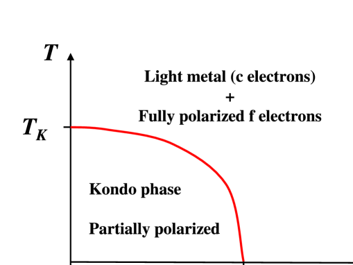
Figure 4: (Color online) Schematic phase diagram of the PAM as a function of a magnetic field $h$. The red solid line indicates $h_{c}(T)$ which separates the trivial $r=0$ solution from the non-trivial one, $r\neq 0$.

Going beyond the linear response, the critical magnetic field $h_{c}(T)$ is defined at a given temperature by the transition between the $r\neq 0$ and $r=0$ state. Solving the MF equations  (12) – (14) in the $r\to 0$ limit and using the definition of the Kondo coupling $J(\mu)$ in Eq.(21), we find for $n_{f}=1$

$$\frac{1}{J(\mu)}=\int_{-\infty}^{+\infty}\frac{\omega}{\omega^{2}-h_{c}^{2}}\rho_{0}(\omega+\mu)\tanh\left[\frac{\omega}{2T}\right]d\omega~{},$$ (38)

which yields $h_{c}\neq 0$ for any regular $\rho_{0}(\omega)$. Unlike the zero-field result, Eq. (22), which is logarithmically singular and gives $J_{c}=0$ for any finite $\rho_{0}(\mu)$, equation (38) yields $J_{c}\neq 0$ for any finite field. For $h\geq h_{c}(T)$, there is only the trivial $r=0$ solution which describes ferromagnetically polarized $f$-moments decoupled from the conduction band (see FIG. 4). For $h\leq h_{c}(T)$, the equations have a non-trivial $r\neq 0$ solution which describes a partially polarized Fermi liquid. At $T=0$, the weak coupling limit ($J\ll D$) yields the universal relation

$$h_{c}^{0}\equiv h_{c}(T=0)=\alpha_{0}^{-1}F_{K}e^{-{1}/{J(\mu)\rho_{0}(\mu)}}=\alpha_{0}^{-1}T_{K}~{}.$$ (39)

Since $\alpha_{0}=1.13$, we have $h_{c}^{0}\simeq T_{K}$. At finite temperatures, the solution of Eq. (38) with constant $c$ DOS yields the critical line

$$[h_{c}(T)/h_{c}^{0}]^{2}+[T/T_{K}]^{2}=1~{},$$ (40)

which separates the trivial solution (the decoupled phase) from the non-trivial one (the FL phase) and holds for any $J(\mu)$ and filling $n$. The critical line $h_{c}(T)$ obtained for a constant $c$ DOS is represented schematically in Fig. 4. The same relation is also found at half-filling, for any $c$ DOS. In general, we expect a ‘nearly’ universal phase boundary, with some small deviations due to the structure of the $c$ DOS and the particle-hole asymmetry.

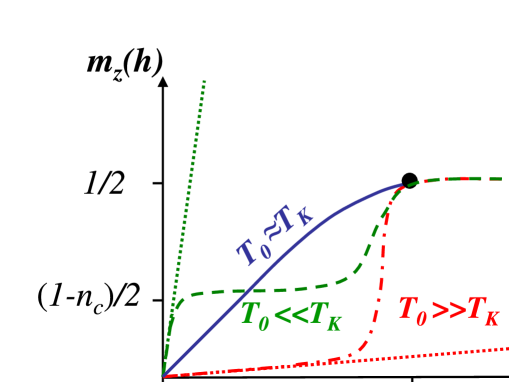
Figure 5: (Color online) Schematic plot of the magnetization $m_{z}$ as a function of reduced magnetic field $h/T_{K}$ for T${}_{0}\gg$T_K (red dash doted line), T${}_{0}\approx$T_K (blue solid line), and T${}_{0}\ll$T_K (green dashed line). The doted lines indicate the initial slope in the linear response regime, where $m_{z}(h)=h/T_{0}$. The black dot refers to the complete polarization of the local $f$ electrons, with $m_{z}=1/2$, which occurs a the critical field $h_{c}^{0}=T_{K}$.

Studying the development of the system as a function of temperature at constant field gives the critical temperature $T_{K}(h)$. Changing the field at constant temperature gives $h_{c}(T)$.

The magnetization $m_{z}(h)$ obtained from the slave boson solution at $T=0$ is plotted in Fig. 5 as a function of reduced magnetic field $h/T_{K}$ for three typical cases: T${}_{0}\ll$T_K, $T_{0}\approx T_{K}$, and $T_{0}\gg T_{K}$. A non-constant $c$ DOS leads to different types of magnetization curves which resemble the temperature dependence of the entropy depicted in Fig. 2 (with the T/T_K axis replaced by $h/h_{c}^{0}$). For $h<\min~{}\{T_{0},T_{K}\}$, the system is in the linear response regime, shown in FIG. 5 by dotted lines; the slope of $m_{z}(h)$ is T_K/T₀, when plotted versus $h/T_{K}$. This regime is analogous to the FL regime described from the entropy. In higher fields, the behavior of the slave boson solution depends on the ratio $T_{0}/T_{K}$. For T${}_{0}\ll$T_K, the $T=0$ magnetization is linear for small fields and then saturates. For $T_{0}<h<T_{K}$, the magnetization might have a plateau which signifies a saturated FL ($r\neq 0$) with a ’large’ FS. At very high fields, $h\geq T_{K}\sim h_{c}^{0}$, the magnetization becomes a universal function of $h/h_{c}^{0}$. In the opposite case, $T_{K}\ll T_{0}$, the low field limit gives $m_{z}(h)\propto h/T_{0}$ and the initial slope appears very small when plotted versus $h/h_{c}^{0}$. Once the field exceeds the critical value, $h_{c}^{0}\sim T_{K}$, the local moments are unscreened and $m_{z}(h)$ rises rapidly towards the free-ion value. Thus, at about $h\simeq h_{c}^{0}$ such systems exhibit a meta-magnetic transition from an unpolarized Fermi liquid to the polarized spin-lattice (the r=0 phase). Of course, this simple considerations should be corrected for direct and indirect effects due to the conducting sea.

II.7 Transport coefficients in the FL regime

The slave boson Hamiltonian in Eq. (4) provides the approximate FL scale T₀ and the low-temperature thermodynamics but has no relaxation mechanisms that could lead to stationary heat and charge currents. To calculate the transport properties of the $SU(N)$ symmetric Anderson model in the $T\to 0$ limit we use the Fermi liquid theoryYamada and Yosida (1986) which takes into account the quasiparticle (QP) damping and leads to a finite relaxation time. The QP excitations of the full model have the same dispersion as the excitations of the MF slave boson model but are restricted to the immediate vicinity of the Fermi level. In the $\omega\to 0$ limit, where the imaginary part of the $f$ electron self energy $~{}\Sigma_{f}(\omega)$ can be neglected, the QP and the slave boson dispersion assume the same form. The correspondence is obtained by identifying $rV$ with $~{}\sqrt{Z_{f}}$ and $\lambda$ with $~{}\tilde{\omega}_{f}$, where $~{}Z_{f}^{-1}=[1-\partial\Sigma_{f}/\partial\omega|_{\omega=0}]$ is the renormalization factor, $~{}\tilde{\omega}_{f}=[E_{f}+{\rm Re}\Sigma_{f}(0)-\mu]Z_{f}$ the renormalized position of the $f$ level, and the excitation energies $\omega$ are measured in both cases with respect to the renormalized chemical potential $\mu$. Unlike the infinitely long-lived MF excitations, which are formally defined for $\omega\leq D-\mu$, the QP excitations are defined for $~{}{\rm Im}~{}\Sigma_{f}(\omega)\ll\omega^{2}$.

We calculate the transport coefficients of the periodic Anderson model with constant hybridization using the fact that the charge and energy current density operators satisfy the Jonson-Mahan theoremEhrenreich and Spaepen (1997). This allows us to express the charge conductivity by $\sigma(T)=e^{2}NL_{11}$, the thermopower by $\alpha(T)|e|T=-L_{12}/L_{11}$, and the electronic contribution to the thermal conductivity by $\kappa(T)T=N(L_{22}-L_{12}^{2}/L_{11})$. In each of these expressions we have introduced the transport integrals:

$$L_{mn}=\int d\omega\left(-\frac{dn_{F}}{d\omega}\right){\omega}^{m+n-2}\Lambda(\omega,T).$$ (41)

where $n_{F}(\omega)=1/[1+\exp(\beta\omega)]$ is the Fermi-Dirac distribution function and $\Lambda(\omega,T)$ is defined by the Kubo linear response theoryMahan (1981). At low temperature $(-dn_{F}/d\omega)$ approaches delta function and the main contribution to the integrals in Eq. (41) comes from the low-energy excitations within the Fermi window, $|\omega|\lesssim T$. In the $\omega,T\rightarrow 0$ limit, a straightforward calculation yields for the three-dimensional systemsZlatić et al. (2008)

$${\Lambda(\omega,T)}=\frac{1}{3}{v^{2}_{F}}\rho_{c}(\omega)\tau(\omega,T),$$ (42)

where we introduced the unrenormalized velocity $v_{\bf k}=-\nabla_{\bf k}\epsilon_{\bf k}$ and denoted by ${v^{2}_{F}}$ the average of $v_{\bf k}^{2}$ over the renormalized Fermi surface of hybridized states. The renormalized $c$ DOS is $\rho_{c}(\omega)$ and the relaxation time is $1/\tau(\omega,T)\simeq~{}{\mathrm{I}m}~{}\Sigma_{c}(\omega)$, where $\Sigma_{c}(\omega)$ is the self energy of the c electrons which must include the quasiparticle damping. The integrals in Eq. (41) are evaluated by the Sommerfeld expansion (for details see Ref. Zlatić et al. (2008)) which yields the transport coefficients of the periodic Anderson model as simple powers of reduced temperature T/T₀. The pre-factors of various powers are functions of $\rho_{0}(\mu_{L})$, $n_{f}$, and $\Delta\mu$ which depend on the local self energy $\Sigma_{f}(\omega)$ which is difficult to obtain for the excitation energies within the Fermi window, $|\omega|\leq T$. To avoid this problems, we replace T₀ and all other renormalized quantities that appear in the FL expressions by the slave boson MF results.

The FL result for the electrical resistivity can be written as Zlatić et al. (2008)

$$R(T) \simeq \frac{9^{2}(\Delta\mu/n_{f})^{2}}{N(N-1)\pi e^{2}{v^{2}_{F}}}(\gamma T)^{2}=\frac{9\pi^{3}(\Delta\mu/n_{f})^{2}~{}T_{K}^{2}}{N(N-1)e^{2}{v^{2}_{F}}~{}T_{0}^{2}}\left(\frac{T}{T_{K}}\right)^{2}=A~{}T^{2}~{},$$ (43)

where $\gamma=(\pi^{2}/6)N\rho(\mu)=\pi^{2}/3T_{0}$ and the in the second equality $R(T)$ is expressed on the reduced temperature scale T/T_K. The coefficient $A=R(T)/T^{2}$ depends not only on specific heat coefficient $\gamma$ but on the difference in the chemical potentials of unhybridized and hybridized Bloch states, the effective degeneracy of the model, and the square of the Fermi velocity averaged over the hybridized FS. This result can be used to explain the pressure- and magnetic field-dependence of $A$, which has been studied experimentally in various systems.

The FL result for the Seebeck coefficient is given for $n_{f}\simeq 1$ by the expression

$${\alpha(T)}=\mp\frac{12~{}\gamma~{}T}{n_{f}|e|}=\mp\frac{4\pi^{2}~{}T_{K}}{n_{f}|e|~{}T_{0}}\frac{T}{T_{K}}~{}.$$ (44)

Since the doubly occupied f states are removed from the Hilbert space, the model is highly asymmetric, and the initial slope $\lim_{T\to 0}\alpha(T)/T$ never vanishes. In bad metals with a low-carrier concentration, $\alpha(T)$ could be very large.

The thermal conductivity in the FL regime reads,

$$\kappa(T)=T\sigma(T){\cal L}_{0}(T)$$ (45)

which yields in the $T\to 0$ limit the Wiedemann-Franz (WF) law, $\kappa(T)\propto\ T\sigma(T)$. However, the usual Lorentz number, ${L}_{0}={\pi^{2}}/{3e^{2}}$, is here replaced by the effective one,

$${\cal L}_{0}(T)=\frac{\pi^{2}}{2e^{2}}\left[1-\frac{32\pi^{2}}{n_{f}^{2}}\left(\frac{T}{T_{0}}\right)^{2}\right]~{}.$$ (46)

The correction given by the square bracket could lead to substantial deviations from the WF law much below T₀, since the factor multiplying the $T^{2}$ term is very large.

III Discussion of the experimental data

The slave boson solution of the periodic Anderson model is used in this Section to discuss the effects of the band structure on the properties of the intermetallic compounds with 4$f$ ions. First, we consider the case of the $c$ DOS with a maximum in the vicinity of the chemical potential, such that the Fermi liquid scale is much smaller than the Kondo scale, T${}_{0}\ll$T_K. These results provide a qualitative explanation of the experiments on YbAl₃ or YbMgAl₄. The opposite case, T${}_{0}\gg$T_K, occurs when the chemical potential is close to the minimum of the $c$ DOS; these results explain the main experimental features of YbInCu₄-like compounds. Finally, for T${}_{0}\simeq$T_K, which seems to characterize CeCu₂Si₂ and CeCu₂Ge₂, we discuss the rapid variation of the $T^{2}$ coefficient of the electrical resistance and of the residual resistance with pressure. The anomalies are related to the pressure-induced change of the effective degeneracy of the $f$ states.

III.0.1 The $T_{0}\ll T_{K}$ case

Unlike the experiments on dilute alloys, the overall temperature dependence of the experimental data on YbAl₃, Yb_1-x Lu_x Al₃ Bauer et al. (2004) for $x\leq 0.05$, YbMgCu₄ and YbCdCu₄Lawrence et al. (2001), cannot be explained by a single energy scale. In these compounds, the high-temperature resistivity is a large and slowly varying function of temperaturevan Daal et al. (1974); Rowe et al. (2002), the thermopowervan Daal et al. (1974); Rowe et al. (2002) has a broad peak around 350 K, the magnetic susceptibility and the specific heat have a broad maximum at $T_{max}\simeq 125$ K, and the Hall coefficient is typical of a metal in which the $c$ electrons scatter on local moments  Cornelius et al. (2002); Bauer et al. (2004). A similar high-temperature behavior is seen in YbXCu₄ (X=Cd, Mg, Zn) Lawrence et al. (2000). The inelastic neutron scattering data on YbAl₃ show a broad Lorentzian spectrum centered at about 540 meV Murani (1985); Osborn et al. (1999), which can be understood in terms of the Kondo effect with T${}_{K}\geq$ 500 K Cornelius et al. (2002). Below 100 K, the electrical resistivity of YbAl₃ decreases due to the formation of a coherent ground state and for $T\leq$T${}_{0}\simeq$ 40 K the resistivity is a parabolic and the thermopower a linear function of temperature  van Daal et al. (1974); Rowe et al. (2002); Ebihara et al. (2000), indicating a Fermi liquid. For $T\leq T_{0}$, the zero-field anomalies in $\chi(T)$ and $C_{V}(T)$ yield an enhanced effective mass Cornelius et al. (2002) of the order of 1/T₀ and the neutron scattering data Murani (1985); Osborn et al. (1999) show a narrow peak at about 30 meV, which is due to a hybridization gap. However, if we plot the low-temperature transport coefficients on a reduced temperature scale T/T_K they appear to be strongly enhanced with respect to the predictions of the single impurity Anderson model with Kondo scale $T_{K}\simeq$ 500 K. Neither the $A$ coefficient of the resistivity nor the slope of the thermopower can be explained by the single impurity c calculations that would capture the main features of the high-temperature data and give $T_{K}\simeq$ 500 K. Optical conductivity at 7 K shows a narrow Drude-like response that is often found in heavy fermion systems Okamura et al. (2003, 2007) and another mid-infrared peak (MIR) that can be associated with the hybridization gap. The optical spectra do not change appreciably for 7 K $\leq$T$\leq$ 40 K, as expected of a system with the characteristic energy scale T${}_{0}\simeq 50$ K. However, the Drude peak broadens and the MIR peak vanishes at higher temperatures. The de Haas - van Alphen experiments performed up to $h\simeq 40$ T, show that the effective mass is reduced along certain directions in k-space by a factor of 2 without a significant alteration of the shape of the Fermi surface Ebihara et al. (2003). The fact that the low-temperature susceptibility anomaly is suppressed in the fields of about 40 T indicates that the high-field mass renormalization and the zero-field anomalies below $T_{0}$ describe different aspects of the same physical state. The low-temperature anomalies are easily destroyed by disorder (they vanish in Yb_1-x Lu_x Al₃ for $x\geq 0.05$), which is another indication that they are related to the coherent state Ebihara et al. (2003).

The overall shape of the experimental data and different characteristic energy scales found at high and low temperatures can be explained by the slave boson solution of the periodic Anderson model close to half-filling. As shown in Secs. II.5 and II.6, if the chemical potential is close to the maximum of the unperturbed $c$ DOS, the mean field equations yield $T_{0}\ll T_{K}\simeq h_{c}^{0}$ and give rise to a ’slow crossover’ from the LM to the FL phase. Taking $T_{0}\simeq 50$ K and $T_{K}\simeq 500$, as suggested by the experiment, we find that the low-temperature susceptibility and the specific heat coefficient are FL-like and much enhanced with respect to the expectations based on the behavior in the incoherent regime. The FL results for the $T^{2}$ term of the resistivity (see Sec. II.7) explain the enhancement that one finds below 50 K when $\rho(T)$ is plotted on the T/T_K scale. The low-temperature thermopower ${\alpha(T)}\propto\left({T_{K}}/{T_{0}}\right){T}/{T_{K}}$ is also enhanced by T${}_{K}/$T₀ with respect to the predictions of the single impurity calculation that reproduce the thermopower maximum above 300 K. For temperatures between T₀ and T_K, the magnetization and the magnetic entropy are reduced with respect to the free-ion value, which is only recovered for $T>T_{K}$. The slave boson solution gives $m_{z}(h)\simeq h/T_{0}$ for $h\ll T_{0}$ and $m_{z}(h)\propto$ const for $h\gg T_{0}$. Since $T_{0}\ll h_{c}^{0}$, the slave boson order parameter is finite for $h\geq T_{0}$, i.e., for $T_{0}\leq h\leq T_{K}$, the system is a polarized heavy FL with a ‘large FS’. Such a behavior explains de Haas – van Alphen data which show that the FS does not change much up to the fields of about 40 T.

The model with the chemical potential close to the maximum in the $c$ DOS describes Yb_1-x Lu_xAl₃ for $x\leq 0.5$. For higher concentrations of Lu there are so many additional holes in the conduction band that the chemical potential shifts away from the peak in the $c$ DOS. In that case, T₀ and T_K approach each other and the ’slow’ crossover does not occur. For $x>0.5$, one can expect a crossover from a lattice regime with T${}_{0}\neq$T_K to a universal dilute regime with T${}_{K}=$T₀, as discussed in RefBurdin and Fulde (2007).

The slave boson dispersion defined by the Hamiltonian in Eq. (4) explains the Drude and the MIR peaks found at 7 K in the optical conductivity. However, we hesitate to discuss the temperature dependence of the hybridization gap using the mean field results. These results are obtained by enforcing the constraint $n_{f}=1$ only on the average, so that the auxiliary fermions are mapped on a free electron gas. The proper redistribution of the spectral weight should not neglect the QP damping and should use the solution which is valid at all energy scales.

III.0.2 The T${}_{0}\gg$T_K case

Unlike YbAl₃ or Yb_1-x Lu_x Al₃ for $x\leq 0.5$, the transition between the LM and the FL phase in Yb_1-x Lu_x Al₃ for $x\geq 0.7$, YbTlCu₄Lawrence et al. (2001), YbInCu₄ and Yb_1-xY_xInCu₄ for $x\leq 0.5$ Sarrao (1999) takes place at temperature T_v in an abrupt way. In YbInCu₄, which we take as a typical example, a first order valence change (VF) transition occurs at ambient pressure at temperature T_v=40 K. Above T_v, the Yb ions are in the 3⁺ configuration and the magnetic response can be understood assuming an independent 4$f$ hole in each unit cell. The ensuing high-temperature effective moment is then close to the free ion value, as observed experimentally. The electrical resistance is very large and nearly temperature independent. The Kondo scale deduced from these data is so much smaller than T_v, that the $f$ and $c$ states are effectively decoupled for T$\geq$T_v. The magnetic fields up to 40 Tesla do not produce any appreciable magnetoresistance which is also an indication of a small Kondo coupling. The large values of the electrical resistance and small Hall constant cannot be explained in terms of the spin disorder scattering but can be taken as an evidence that the $c$ DOS has a pseudogap or a deep minimum in the immediate vicinity of the chemical potential. When the compound is cooled down to temperature T_v, the lattice expands and the Yb configuration changes from 3⁺ to 2.9⁺. In the VF phase, the susceptibility and the specific heat coefficientare moderately enhanced ($\gamma\simeq 50$ mJ/mol K), the resistivity is quadratic and the thermopower linear in temperature. The ratio $\alpha/T\gamma$ is typical of a normal FLBehnia et al. (2004) but the Kadowaki-Woods ratio is anomalously low. The characteristic energy scale in the VF phase is much larger than T_v; the data give $T_{0}\approx 500$ K Dallera et al. (2002). The optical conductivityGarner et al. (2000), the Hall effectFigueroa et al. (1998), and the thermoelectric powerOčko and Sarrao (2002) indicate that a bad metal with only a few states close to the chemical potential is transformed at T_v into a good metal with small $\gamma$. That is, the VF transition is accompanied by a major reconstruction of the conduction states.

An application of pressure shifts $T_{v}(P)$ to lower temperatures Mito et al. (2003); Mitsuda et al. (2004); Park et al. (2006); Mito et al. (2007) without changing the properties of the high-temperature state. For $T\geq T_{v}(P)$, the susceptibility and the specific heat of YbInCu₄ can be explained by the crystal field (CF) theory of independent $f$ statesAviani and et al. (2008) split by $\Delta_{CF}\simeq$ 40 K into an excited quartet and two nearly degenerate doublets. This CF scheme agrees with the neutron scattering dataSevering and et al. (1990). The entropy of the LM phase, obtained by integrating $C_{V}(T)/T$ Park et al. (2006); Aviani and et al. (2008), decreases from $S\simeq R\ln 8$ to $S\simeq R\ln 4$ as the system is cooled down to $T_{v}(P)$, as expected for two CF quartets without any Kondo screening. This indicates, once again, that the Kondo scale of the LM phase is much smaller than $T_{v}(P)$. Pressure stabilizes the paramagnetic phase and at a critical pressure of $P_{c}=$ 2.5 GPa the LM persists down to $T_{c}=$ 2.5 K, where the magnetic transition removes the paramagnetic entropy of about $S\simeq R\ln 4$. The NMR Mito et al. (2003, 2007) and neutron scattering data show that the local moments in the magnetically ordered (MO) phase are somewhat smaller than in the LM phase just above $T_{N}$. Since the specific heat coefficient and the $A$ coefficient of the resistivity are much larger for $P\geq P_{c}$ than for $P\leq P_{c}$, we speculate that the transition in the MO phase is accompanied by an increase of Kondo coupling. As regards the doping, replacing Yb with Y or Lu ionsZhang et al. (2002); Mitsuda et al. (2004) produces similar effects as pressure, i.e., doping stabilizes the LM configuration and shifts $T_{c}$ to lower temperatures. In Eu-based intermetallics, the valence-change transition exhibits similar features Wada et al. (1997); Mitsuda et al. (2000) as in YbInCu₄, except T_v is higher ($T_{v}\geq 100$ K) and the valence state of Eu ions changes almost completely [from $2^{+}$ ($f^{7}$) to $3^{+}$ ($f^{6}$)].

We close this experimental summary by mentioning that the VF transition shifts in an magnetic field to lower tempeatures. At ambient pressure, the critical field of $h_{c}^{0}\simeq 40$ Tesla suppresses the VF transition and removes completely the FL statate of YbInCu₄. The experiments give $\mu_{eff}h_{c}^{0}=T_{v}$, where $\mu_{eff}$ is the effective magnetization of the 4$f$ state in the LM regime, i.e., at the VF transition, the magnetic energy of the paramagnetic $f$ states is comparable to the Kondo energy of the FL phase. The critical field is temperature dependent and the phase boundary between the LM phase and the FL phase is given by the expression $h_{c}(T)=h_{c}^{0}\sqrt{1-(T/T_{v})^{2}}$, where $h_{c}^{0}$ is the zero-temperature value.

The aforementioned behavior of YbInCu₄ and similar systems can be understood from the slave boson solution of the periodic Anderson model. Taking the chemical potential of the high-temperature phase close to the pseudo-gap of the unrenormalized $c$ DOS we find a very smal Kondo temperature (see Sec. II.3), which explains the Curie-like susceptibility, a large and nearly temperature-independent resistivity, small thermopower, and a negligible magnetoresistance observed for $T\geq T_{v}$. Since the Kondo screening is absent in the LM phase, we can neglect the hybridization altogether and discuss the high-temperature properties of YbInCu₄ by adding the Falicov-Kimball term to the effective Hamiltonian. This term opens a gap or a pseudogap in the excitation spectrumFreericks and Zlatić (1998) and explains most of the qualitative features in a self-consistent way. For a quantitative description of the paramagnetic phase, one would have to include the corrections due to the CF splitting of the $f$ statesFreericks and Zlatić (2003).

The peculiar feature of YbInCu₄ and similar systems is that the local moments remain unscreened down to very low temperatures. System with a pseudogap in the $c$ DOS cannot remove the paramagnetic entropy by Kondo effect but have to approach the ground state by an entirely different route. In YbInCu₄ the transition into a low-etropy state is achieved by an iso-structural phase transition which expands the lattice and facilitates the valence fluctuations between xthe low-volume 4$f^{13}$ and the large-volume 4$f^{14}$ state of Yb. The presence of the 4$f^{14}$ configuration in the ground state means that some $f$ holes are transferred in the $c$ band, so that the chemical potential is shifted away from the pseudogap. This increases the Kondo coupling and makes the Kondo temperature of the expanded lattice comparable to T_v. For $T\leq T_{K}$, the local moment disappears, because the $f$ and $c$ states form hybridized bands, i.e., the $f$ holes participate in the Fermi volume. The $f$–$c$ charge transfer induced by hybridization stabilizes the low-entropy FL state and compensates the loss of elastic energy due to the lattice expansion. Once the Kondo scale of the hybridized system is equal to T_v, the expansion terminates, as can be seen from the following argument. The VF transition takes place at T_v, where the free energy of the high-temperature phase, ${\cal F}_{LM}$, is equal to the free energy of the low-temperature (expanded) phase, ${\cal F}_{FL}$. Below T_v, the free energy is dominated by the hybridization term in the internal energy which stabilizes the FL state, ${\cal F}_{FL}<{\cal F}_{LM}$. Above T_v, where the free energy is dominated by the paramagnetic entropy, the local moments of the pseudogapped phase are completely free, while in the expanded lattice they would be partially screened. Since the free energy of the expanded lattice would be bigger than ${\cal F}_{LM}$, the most stable configuration above T_v is the low-volume (paramagnetic) one.

In the expanded lattice, the chemical potential is still rather close to the minimum of the $c$ DOS, which makes the FL scale much larger than the Kondo scale T_v (see Sec. II.4). If we estimate the FL corrections to the $T=0$ value of the magnetic susceptibility or the electric resistivity up to ${\cal O}[(T/T_{0})^{2}]$ and assume $T_{0}/T_{K}\leq 10$ (as indicated by the data), the maximum relative deviation at $T\sim T_{v}$ is $1$%. The Kadowaki-Woods ratio in the FL phase is anomalously small, because the CF splitting does not affect the delocalized $f$ states, so that the $f$ states are effectively 8-fold degenerate. The FL analysis presented in Sec. III.3, shows that the $A$ coefficient is then reduced by a factor $1/N(N-1)$. Thus, the slave boson theory provides an overall description of YbInCu₄-like compounds at ambient pressure.

To account for the effects of pressure, we recall that pressure stabilizes the low-volume (4$f^{13}$) configuration with respect to the large-volume (4$f^{14}$) one and model this effect by shifting the $f$ level away from the chemical potential. This reduces the $f$–$c$ coupling and the Kondo scale, shifts T_v to lower temperatures and removes eventually the VF transition. For very large pressures, the paramagnetic entropy of the LM phase is not removed by the the lattice expansion but by a transition into a magnetically ordered (MO) phase which takes place at Curie temperature $T_{c}$.

In the presence of an external magnetic field, the condition for the phase boundary, ${\cal F}_{LM}(T,h)={\cal F}_{FL}(T,h)$, can be approximated by the condition $S_{LM}(T_{v},h)=$ const., where $S_{LM}(T_{v},h)$ is the entropy of the LM phaseDzero et al. (2000). This approximation uses the fact that T₀ is not affected by the pseudo-gap, so that $T_{0}\gg T_{v}$, and the temperature and the field-dependence of ${\cal F}_{FL}$ can be neglected for $T\leq$T${}_{v}(h)$. The critical line obtained in such a way agrees very well with the experimental dataDzero (2002); Freericks and Zlatić (2003) and with the slave boson result given by Eq. (40). For large fields, the slave boson solution shown by the dashed-doted curve in Fig.5 explains the metamagnetic transition that takes place at the critical field, $h_{c}^{0}\propto T_{v}$.

Similar reasoning explains also the unusual behavior of the newly reported system Yb₃Pt₄ Kobayashi and et al (2007); Bennett et al. (2008). In the paramagnetic phase Yb₃Pt₄ has the Curie-like susceptibility and nearly constant resistivity which exceeds the spin-disorder limit. Like in YbInCu₄, the LM phase of Yb₃Pt₄ looks semimetallic, with unrenormalized (’light’) Bloch sates and localized $f$ states. In the absence of the $f$–$c$ exchange coupling, the paramagnetic entropy cannot be reduced by the Kondo screening but the ground state has to be approached by an alternative route. In Yb₃Pt₄ the ground state is magnetic and we speculate that the LRO is due to a spin density wave (SDW). The transition between the LM and the SDW phase takes place at $T_{N}\simeq 2$ K. The data show that the effective mass of metallic electrons becomes heavy at $T_{N}$ Bennett et al. (2008).

This behavior can be explained by the slave boson approach, assuming that the chemical potential is close to the pseudo gap of the unperturbed $c$ band and admitting an AFM solution. The generalized slave boson equations which include the coupling to the staggered magnetization provide at $T_{N}$ a non-trivial solution with hybridized states and a large FS. The reason is that large internal fields shift the chemical potential of up and down spins away from the singularity in $c$ DOS (like in the case of an external magnetic field, discussed in section II.6). Since the Kondo coupling in the LM phase is very small, the $c$ electrons are nearly free and the Kondo screening can only occur at extremely low temperatures. Unlike YbInCu₄, where the paramagnetic entropy is removed by an iso-structural phase transition which enables hybridization and the transition to the FL phase, in Yb₃Pt₄ the paramagnetic entropy is removed by a spin density wave (SDW) transition which partially gaps the Fermi surface. The formation of the SDW at temperature $T_{N}\simeq$ 2 K switches-on the hybridization, which delocalizes the $f$ states, changes the effective degeneracy of the $f$ states, and renormalizes the metallic mass. The chemical potential in the SDW phase is still rather close to the pseudo-gap, so that the ensuing FL scale is large, $T_{0}\gg T_{N}$ (see discussion in Sec. II.4). Hence, the mass enhancement at the transition is moderate or small. It would be interesting to check the assumption about the pseudogap in the $c$ DOS by performing the band structure calculations that would take into account the large Coulomb repulsion between the $f$ electrons.

III.0.3 The $T_{0}\simeq T_{K}$ case

As a final example we consider the anomalous pressure dependence of the $T^{2}$ coefficient of the resistivity, $A(P)$, and the residual resistance, $\rho_{0}(P)$, observed in heavy fermions like CeCu₂Si₂Holmes et al. (2004), CeCu₂Ge₂Jaccard et al. (1999) or CePd₂Ge₂Wilhelm and Jaccard (2002) at very low temperatures. In these compounds, the FL scale is about the same as the Kondo scale inferred from the low-temperature peak in $\rho(T)$ or $\alpha(T)$Jaccard et al. (1999); Zlatić et al. (2008). The scales T₀ and T_K are much smaller than the CF splitting (estimated from the high-temperature peak in in $\rho(T)$ or $\alpha(T)$Zlatić et al. (2008)), so that the excited CF sates can be neglected for $T\leq$T${}_{K}\ll\Delta_{CF}$. At ambient pressure, the ground state of these compounds is often superconducting or magnetic and the FL behavior is enforced by applying an initial pressure $P_{0}$. For $P>P_{0}$, the data show that $A(P)$ decreases gradually from large initial values, drops at a critical pressure $P_{c}$ by nearly two orders of magnitudeJaccard et al. (1999); Wilhelm and Jaccard (2002); Holmes et al. (2004), and then continues a gradual decrease. The residual resistance increases from a small initial value, rises rapidly to a sharp peak at $P_{c}$, and decreases at very high pressure to rather small valuesJaccard et al. (1999); Holmes et al. (2004).

We explain these features by assuming that for $P_{0}\leq P\leq P_{c}$ the effective degeneracy of the model is defined by the lowest CF state and that pressure changes the $f$–$c$ coupling and T_K but not $\Delta_{CF}$. The FL state established at $P_{0}$ has a large Fermi surface, because the $f$ electrons are delocalized and participating in the Fermi sea. Taking, for simplicity, the half-filled conduction band and describing the 4$f$ state be a CF doublet, we find that the Fermi surface is close to the edge of the Brillouin zone and that the average Fermi velocity in Eq. (43) is small. In the aforementioned compounds the FL scale is small, so that $A(P_{0})$ large. As long as pressure does not change the degeneracy of the $f$ states, Luttinger theorem preserves the Fermi surface, so that $v_{F}^{2}$ and ${{\Delta\mu}}$ in Eq. (43 ) remain approximately constant. Since $N$ is also constant in this pressure range, the pre-factor of the $(\gamma T)^{2}$-term in Eq. (43) does not change much. Thus, the main effect of pressure is a gradual reduction of $A(P)$ from the maximum value attained at $P_{0}$. This reduction is due to the increase of $T_{0}(P)$, as can be seen from the linear scaling between $\sqrt{A(P)}$ and the inverse Kondo scale of the system $1/$T${}_{K}(P)$Jaccard et al. (1999).

At large enough pressure the hybridization becomes too large for the system to support the CF excitations, so that the effective degeneracy of the ground state increases. For $P\geq P_{c}$, the degeneracy is not set by the lowest CF level but by the full multiplet (a sextet, in the case of Cerium). The slave boson solution of the periodic Anderson model with the $SU(N)$ symmetry and infinite correlation shows that the Fermi volume decreases as $N$ increases, because a single $f$ electron has to be distributed over more and more channels. The chemical shift ${{\Delta\mu}}$ and the specific heat coefficient $\gamma$ also decrease with $N$, while $v^{2}_{F}$ becomes larger on a smaller FS, so that $A(P)$ drops sharply for $P\geq P_{c}$. The degeneracy of the $f$ state does not change for $P>P_{c}$ and an increase of pressure above $P_{c}$ reduces $A(P)$ by increasing T₀. In this pressure range, we find the scaling between ${A(P)}$ and $1/$T${}_{K}^{2}$, where T${}_{K}^{2}$ is the Kondo scale of the $N$-fold degenerate model.

The residual resistance also tracks the pressure-induced changes in the effective degeneracy. If the $f$ states are localized at ambient pressure, as seems to be the case with CeCu₂Ge₂Jaccard et al. (1999) or CePd₂Ge₂Wilhelm and Jaccard (2002) at very low temperatures, the initial values of $\rho_{0}(P_{0})$ are small. Taking, for simplicity, the model with a ground state doublet and an excited CF quartet, and using the FL laws, we find that the temperature dependence of the resistivity at ambient pressure is due to two resonant channels, while most of the current is carried by four non-resonant channels which have temperature-independent conductivity. The contribution of the resonant channels to the residual resistance can be neglected. At large enough pressure, $P\simeq P_{c}$, the CF excitations are removed, the degeneracy of the ground state changes from doublet to sextet, and all the channels become resonant. Because of Luttinger theorem, the Fermi volume shrinks for two of the channels (former resonant ones) and expands for four of them (former non-resonant ones). Hence, for $P\simeq P_{c}$, the overall contribution to the residual resistance increases sharply. A further increase of pressure does not change the degeneracy of the model but gives rise to the charge transfer from the $f$ to the $c$ states. This reduces the residual resistance and gives the $\rho_{0}(P)$ curve its asymmetric shape. In other words, the FL liquid laws and the slave boson solution of the periodic Anderson model show that the large peaks in $A(P)$ and $\rho_{0}(P)$ are due to the pressure-induced change in the degeneracy of the $f$ state.

IV Summary and conclusions

It is well known that the degeneracies and the splittings of the 4$f$ states have a strong impact on the Kondo scale and the high-temperature behavior of intermetallic compounds with Ce, Eu or Yb ions. In this paper, we have shown that the details of the conduction electron band structure have a large impact on the ratio of the Kondo scale to the Fermi liquid scale, which determines the type of the crossover between the incoherent and coherent regimes.

Our analysis is based on the periodic Anderson model, which can be mapped at high temperatures on a single impurity Anderson or Kondo models with Kondo scale T_K. The incoherent properties of the lattice can be understood using a single impurity approximation which takes into account the structure of the $f$ states. At low temperatures, the slave boson solution of the periodic model yields the FL laws characterized by an energy scale T₀. The Kondo and the FL scales depend on the shape of the $c$ DOS in the vicinity of the chemical potential, the degeneracy and the CF splitting of the $f$ states, the number of $c$ and $f$ electrons, and their coupling. The ratio T${}_{0}/$T_K is determined by the details of the band structure. Depending on the relative magnitude of T₀ and T_K, the crossover between the high- and low-temperature regimes proceeds along very different routes. A sharp peak in the $c$ DOS yields T${}_{0}\ll$T_K and gives rise to a ’slow crossover’, as observed in YbAl₃ and similar compounds. The minimum in the $c$ DOS yields T${}_{0}\gg$T_K, which causes an abrupt transition between the high- and low-temperature regimes, as observed in YbInCu₄-like systems. In the case of CeCu₂Ge₂ and CeCu₂Si₂, where T${}_{0}\simeq$T_K, our results show that the pressure-dependence of the $A(P)$ coefficient and the residual resistance can be related to the change in the degeneracy of the $f$ states.

The slave boson solution shows that the low-temperature response of the periodic model can be enhanced (or reduced) with respect to the predictions of the single-impurity model with the same Kondo scale. In the coherent regime, the renormalization of transport coefficients modifies the Wiedemann-Franz law and can lead to an enhancement of the thermoelectric figure-of-merit. The FL laws explain the correlation between the specific heat coefficient $\gamma$ and the slope of the thermopower, $\alpha(T)/T$, or between $\gamma$ and the T² coefficient of the electrical resistance $A=\rho(T)/T^{2}$. In the case of a $N$-fold degenerate model, the FL laws explain the deviations of the Kadowaki-Woods ratio $R_{KW}=A/\gamma^{2}$ and the $q$ ratio, $q=|e|lim_{\{T\to 0\}x}\alpha/\gamma T$, from the universal values.

The shape of the $c$ DOS affects also the magnetic response of the system. The field-dependence of the magnetization resembles the temperature-dependence of the entropy, as can be seen from Figs. 5 and  2. The $c$ DOS with a maximum around the chemical potential leads to an extended plateau in $m(h)$, while a pseudo-gap in the $c$ DOS leads to a metamagnetic transition for the fields of the order of the Kondo temperature.

Appendix A Generalization to multi-orbital systems

A.1 General formalism

Here, we generalize our model to more realistic systems where the local f orbital have a supplementary degeneracy. The later is lift at low temperature by the crystal field. In the limit $U\to\infty$, the PAM Hamiltonian (2) is generalized to

$$H=\sum_{{\bf k}\sigma}\epsilon_{\bf k}c_{{\bf k}\sigma}^{\dagger}c_{{\bf k}\sigma}+\sum_{i\alpha\sigma}(E_{f}+\Delta_{CF}^{\alpha})f_{i\alpha\sigma}^{\dagger}f_{i\alpha\sigma}+V\sum_{i\alpha\sigma}[c_{i\sigma}^{\dagger}f_{i\alpha\sigma}+f_{i\alpha\sigma}^{\dagger}c_{i\sigma}]-\mu\sum_{i\sigma}\left[\sum_{\alpha}f_{i\alpha\sigma}^{\dagger}f_{i\alpha\sigma}+c_{i\sigma}^{\dagger}c_{i\sigma}\right]~{},$$ (47)

where $\alpha=1,\cdots,N/2$ is a local orbital index, and $\Delta_{CF}^{\alpha}$ is the crystal field. For Ce and Yb we have $N=6$ and $N=8$. The slave boson approach described in section II for $N=2$ can be easily generalized within the mapping $\left|0\right>_{i}^{f}\longrightarrow b_{i}^{\dagger}\left|0\right>_{i}$, $\left|\alpha\sigma\right>_{i}^{f}\longrightarrow d_{i\alpha\sigma}^{\dagger}\left|0\right>_{i}$, with the exclusion of all the states with more than one electron on a given site. This leads to the local identities $b_{i}^{\dagger}b_{i}+\sum_{\alpha\sigma}f_{i\alpha\sigma}^{\dagger}f_{i\alpha\sigma}=1$, which are satisfied by introducing Lagrange multipliers $\lambda_{i}$. Within the mean-field approximation, we replace the bosonic fields $b_{i}$ and the Lagrange multipliers $\lambda_{i}$ by homogeneous static real fields $r$, and $\lambda$. The quadratic mean-field Hamiltonian (4) obtained for $N=2$ is then generalized to

$$H=\sum_{{\bf k}\sigma}\left[{\epsilon_{\bf k}c_{{\bf k}\sigma}^{\dagger}c_{{\bf k}\sigma}+rV\sum_{\alpha}\left({c_{{\bf k}\sigma}^{\dagger}d_{{\bf k}\alpha\sigma}+d_{{\bf k}\alpha\sigma}^{\dagger}c_{{\bf k}\sigma}}\right)-\mu c_{{\bf k}\sigma}^{\dagger}c_{{\bf k}\sigma}+\sum_{\alpha}(\lambda+\Delta_{CF}^{\alpha})d_{{\bf k}\alpha\sigma}^{\dagger}d_{{\bf k}\alpha\sigma}+\frac{E_{f}-\lambda-\mu}{2}(1-r^{2})}\right]~{}.$$ (48)

The self-consistent parameters $r$ and $\lambda$ are obtained by minimizing the free energy $\beta{\cal F}(r,\lambda)\equiv-\ln Tre^{-\beta H}$, such that ${\partial{\cal F}(r,\lambda)}/{\partial r}=0$ and ${\partial{\cal F}(r,\lambda)}/{\partial\lambda}=0$. This gives

$$2r(E_{f}-\lambda-\mu) = V\sum_{{\bf k}\alpha\sigma}\langle c_{{\bf k}\sigma}^{\dagger}d_{{\bf k}\alpha\sigma}+d_{{\bf k}\alpha\sigma}^{\dagger}c_{{\bf k}\sigma}\rangle~{},$$ (49)

$$r^{2} = 1-\sum_{{\bf k}\alpha\sigma}\langle d_{{\bf k}\alpha\sigma}^{\dagger}d_{{\bf k}\alpha\sigma}\rangle~{},$$ (50)

where, $\langle\cdots\rangle$ denotes the thermal average with respect to the mean-field Hamiltonian (48) and

$$n=\sum_{i\sigma}\langle\sum_{\alpha}d_{i\alpha\sigma}^{\dagger}d_{i\alpha\sigma}+c_{i\sigma}^{\dagger}c_{i\sigma}\rangle\equiv\sum_{\alpha}n_{f}^{\alpha}+n_{c}~{}.$$ (51)

The average electronic occupation per site of the $f$ and $c$ orbitals is $n_{f}^{\alpha}\equiv\sum_{i\sigma}\langle f_{i\alpha\sigma}^{\dagger}f_{i\alpha\sigma}\rangle=\sum_{i\sigma}\langle d_{i\alpha\sigma}^{\dagger}d_{i\alpha\sigma}\rangle$ and $n_{c}\equiv\sum_{i\sigma}\langle c_{i\sigma}^{\dagger}c_{i\sigma}\rangle$, respectively. These averages are determined by the slave-boson amplitude and the total electronic occupation,

$$\sum_{\alpha}n_{f}^{\alpha} = 1-r^{2}~{},$$ (52)

$$n_{c} = n-\sum_{\alpha}n_{f}^{\alpha}~{}.$$ (53)

The self-consistent Eqs. (49, 50, 51) can be rewriten as

$$r\frac{E_{f}-\lambda-\mu}{2} = -V\int_{-\infty}^{+\infty}\rho_{dc}(\omega)n_{F}(\omega)d\omega~{},$$ (54)

$$\frac{n_{f}^{\alpha}}{2} = \int_{-\infty}^{+\infty}\rho_{d}^{\alpha}(\omega)n_{F}(\omega)d\omega~{},$$ (55)

$$\frac{n_{c}}{2} = \int_{-\infty}^{+\infty}\rho_{c}(\omega)n_{F}(\omega)d\omega~{},$$ (56)

where $n_{F}(\omega)\equiv 1/[1+e^{\beta\omega}]$ is the Fermi function and $\rho_{dc}$, $\rho_{d}^{\alpha}$ and $\rho_{c}$ are the spectral densities of the local single-particle Green’s functions of a given spin. These Green’s functions are defined in the usual way as thermal averages of the (imaginary) time-ordered products of the appropriate creation and annihilation operators.

$$\rho_{dc}(\omega) \equiv -\frac{1}{\pi}\sum_{{\bf k}}\sum_{\alpha}{\mathrm{I}m}\ G_{dc}^{\alpha}({\bf k},\omega)~{},$$ (57)

$$\rho_{d}^{\alpha}(\omega) \equiv -\frac{1}{\pi}\sum_{{\bf k}}{\mathrm{I}m}\ G_{d}^{\alpha}({\bf k},\omega)~{},$$ (58)

$$\rho_{c}(\omega) \equiv -\frac{1}{\pi}\sum_{{\bf k}}{\mathrm{I}m}\ G_{c}({\bf k},\omega)~{}.$$ (59)

The Green functions are computed from the quadratic Hamiltonian (48). We find

$$G_{cc}({\bf k},\omega) = \frac{1}{\omega+\mu-\epsilon_{\bf k}-r^{2}V^{2}\sum_{\alpha}1/(\omega-\lambda-\Delta_{CF}^{\alpha})}~{},$$ (60)

$$G_{dc}^{\alpha}({\bf k},\omega) = -\frac{rV}{\omega-\lambda-\Delta_{CF}^{\alpha}}G_{cc}({\bf k},\omega)~{},$$ (61)

$$G_{dd}^{\alpha}({\bf k},\omega) = \frac{1}{\omega-\lambda-\Delta_{CF}^{\alpha}}+\frac{r^{2}V^{2}}{(\omega-\lambda-\Delta_{CF}^{\alpha})^{2}}G_{cc}({\bf k},\omega)~{}.$$ (62)

We define the non-interacting electron Green’s function

$$G_{0}(\omega)\equiv\sum_{\bf k}\frac{1}{\omega-\epsilon_{\bf k}}~{}.$$ (63)

The local spectral densities can be rewritten as

$$\rho_{c}(\omega) = -\frac{1}{\pi}{\mathrm{I}m}\ G_{0}\left(\omega+\mu-r^{2}V^{2}\sum_{\alpha}\frac{1}{\omega-\lambda-\Delta_{CF}^{\alpha}}\right)~{},$$ (64)

$$\rho_{dc}^{\alpha}(\omega) = \frac{1}{\pi}{\mathrm{I}m}\ \left[\frac{rV}{\omega-\lambda-\Delta_{CF}^{\alpha}}G_{0}\left(\omega+\mu-r^{2}V^{2}\sum_{\alpha}\frac{1}{\omega-\lambda-\Delta_{CF}^{\alpha}}\right)\right]~{},$$ (65)

$$\rho_{d}^{\alpha}(\omega) = -\frac{1}{\pi}{\mathrm{I}m}\ \left[\frac{1}{\omega-\lambda-\Delta_{CF}^{\alpha}}+\frac{r^{2}V^{2}}{(\omega-\lambda-\Delta_{CF}^{\alpha})^{2}}G_{0}\left(\omega+\mu-r^{2}V^{2}\sum_{\alpha}\frac{1}{\omega-\lambda-\Delta_{CF}^{\alpha}}\right)\right]~{}.$$ (66)

A.2 Degenerate case: no crystal field splitting

We consider here $\Delta_{CF}^{\alpha}=0$. In this case, we can check easily that the complete formalism described in this article for $N=2$ can be generalized to any value of $N$, within the following rescaling

$$V^{2}\longrightarrow\frac{N}{2}V^{2}~{}.$$ (67)

Note that, due to the exponential dependence of the energy scales $T_{0}$ and T_K with respect to $V^{2}$ (see Eqs. (21-23-35), these two scales have to be rescaled like

$$T_{K}^{(N)}=T_{K}^{(2)}e^{-(2-N)/NJ(\mu_{0})\rho_{0}(\mu_{0})}~{},$$ (68)

$$T_{0}^{(N)}=T_{0}^{(2)}e^{-(2-N)/NJ(\mu_{0})\rho_{0}(\mu_{0})}~{},$$ (69)

where $(N)$ refers to the number of degenerate channels considered for the $f$ orbitals.

A.3 Kondo temperature

For $r\to 0$, the generalized mean-field equations can be written as

$$\frac{n_{c}}{2} = \int_{-\infty}^{+\infty}\rho_{0}(\omega+\mu)n_{F}(\omega)d\omega~{},$$ (70)

$$\frac{n_{c}^{\alpha}}{2} = n_{F}(\lambda+\Delta_{CF}^{\alpha})~{},$$ (71)

$$\frac{E_{f}-\lambda-\mu}{V^{2}} = \sum_{\alpha=1}^{N/2}\int_{-\infty}^{+\infty}\frac{1}{\omega-\lambda-\Delta_{CF}^{\alpha}}\rho_{0}(\omega+\mu)\tanh\left(\frac{\omega}{2T}\right)d\omega~{}.$$ (72)

We can arbitrarily choose one vanishing $\Delta_{CF}^{\alpha=0}=0$, corresponding to the doublet with the lowest local energy $E_{f}$. If, for the other doublets, one has $\Delta_{CF}^{\alpha\neq 0}>>T$, then we obtain $n_{f}^{\alpha\neq 0}=0$, and the formalism developed for $N=2$ can be applied simply. In the more general case where $\Delta_{CF}^{\alpha\neq 0}\sim T$, or $\Delta_{CF}^{\alpha\neq 0}<T$ then one has to consider also the contribution from these orbitals.

References

- Anderson (1970) P. W. Anderson, J. Phys.C 3, 2346 (1970).
- Wilson (1975) K. G. Wilson, Rev. Mod. Phys. 47, 733 (1975).
- Nozières (1974) P. Nozières, J. Low. Temp. Phys. 17, 37 (1974).
- Yamada (1975) K. Yamada, Prog. Theor. Phys. 53, 970 (1975).
- Tsvelick and Wiegmann (1983) A. Tsvelick and P. Wiegmann, Adv. Phys 32, 453 (1983).
- Withoff and Fradkin (1990) D. Withoff and E. Fradkin, Phys. Rev. Lett. 64, 1835 (1990).
- Vojta and Bulla (2002) M. Vojta and R. Bulla, Phys. Rev. B. 65, 014511 (2002).
- Sheehy and Schmalian (2008) D. E. Sheehy and J. Schmalian, Physical Review B 77, 125129 (2008).
- Bauer et al. (2004) E. D. Bauer, C. H. Booth, J. M. Lawrence, M. F. Hundley, J. L. Sarrao, J. D. Thompson, P. S. Riseborough, and T. Ebihara, Physical Review B (Condensed Matter and Materials Physics) 69, 125102 (pages 8) (2004).
- Sarrao (1999) J. L. Sarrao, Physica B 259 & 261, 129 (1999).
- Wada et al. (1997) H. Wada, A. Nakamura, A. Mitsuda, M. Shiga, T. Tanaka, H. Mitamura, and T. Goto, 9, 7913 (1997).
- Mitsuda et al. (2000) A. Mitsuda, H. Wada, M. Shiga, and T. Tanaka, J. Phys.: Condens. Matter 12, 5287 (2000).
- Barnes (1976) S. Barnes, J. Phys.F: Met. Phys. 6, 1375 (1976).
- Coleman (1984) P. Coleman, Phys. Rev. B 29, 3035 (1984).
- Zlatić et al. (2007) V. Zlatić, R. Monnier, J. Freericks, and K. W. Becker, Phys. Rev. B 76, 085122 (2007).
- Burdin et al. (2000) S. Burdin, A. Georges, and D. R. Grempel, Phys. Rev. Lett. 85, 1048 (2000).
- Zlatić et al. (2008) V. Zlatić, R. Monnier, and J. Freericks, Phys. Rev. B 78, 045113 (2008).
- Tahvildar-Zadeh et al. (1997) A. N. Tahvildar-Zadeh, M. Jarrell, and J. K. Freericks, Phys. Rev. B 55, R3332 (1997).
- Nozières (1985) P. Nozières, Ann. Phys. (Paris) 10, 19 (1985).
- Nozières (1986) P. Nozières, Eur. Phys. B 6, 447 (1986).
- Mahan (1981) G. D. Mahan, Many-Particle Physics (Plenum, New York, 1981).
- Yamada and Yosida (1986) K. Yamada and K. Yosida, Prog. Theor. Phys. 76, 681 (1986).
- Ehrenreich and Spaepen (1997) H. Ehrenreich and F. Spaepen, Good Thermoelectrics (Academic Press, San Diego, 1997), vol. 51 of Solid State Physics, chap. G. D. Mahan, p. 81.
- Lawrence et al. (2001) J. M. Lawrence, P. S. Riseborough, C. H. Booth, J. L. Sarrao, J. D. Thompson, and R. Osborn, Phys. Rev. B 63, 054427 (2001).
- van Daal et al. (1974) H. J. van Daal, P. B. van Aken, and K. H. J. Buschow, Phys. Lett. A 49, 246 (1974).
- Rowe et al. (2002) M. Rowe, V. L. Kuznetsov, L. A. Kuznetsova, and G. Min, J. Phys.D: Applied Physics 35, 2183 (2002).
- Cornelius et al. (2002) A. Cornelius, J. Lawrence, T. Ebihara, P. Riseborough, C. Booth, M. Hundley, P. Pagliuso, J. S. andJ.D.Thompson, M. Jung, A. Lacerda, et al., Physical Review Letters 88, 117201 (2002).
- Lawrence et al. (2000) J. M. Lawrence, P. Riseborough, C. Booth, J. L. Sarrao, J. D. Thompson, and R. Osborn, Physical Review B (Condensed Matter and Materials Physics) 63, 054427 (2000).
- Murani (1985) A. Murani, Physical Review Letters 54, 1444 (1985).
- Osborn et al. (1999) R. Osborn, E. Goremychkin, I. Sashin, , and A. Murani, J. Appl. Phys. 85, 5344 (1999).
- Ebihara et al. (2000) T. Ebihara, Y. Inada, M. Murakawa, S. Uji, C. Terakura, T. Terashima, E. Yamamoto, Y. Haga, Y. Onuki, and H. Harima, J. Phys. Soc. Jpn. 69, 895 (2000).
- Okamura et al. (2003) H. Okamura, T. Ebihara, , and T. Nanba, Acta Phys. Pol. B 24, 1075 (2003).
- Okamura et al. (2007) H. Okamura, T. Watanabe, M. Matsunami, T. Nishihara, N. Tsujii, T. Ebihara, H. Sugawara, H. Sato, Y. ?nuki, Y. Isikawa, et al., J. Phys. Soc. Jpn. 76, 023703 (2007).
- Ebihara et al. (2003) T. Ebihara, E. Bauer, A. Cornelius, J. Lawrence, N. Harrison, J. Thompson, J. Sarrao, M. Hundley, and S. Uji, Physical Review Letters 90, 166404 (2003).
- Burdin and Fulde (2007) S. Burdin and P. Fulde, Phys. Rev. B 76, 104425 (2007).
- Behnia et al. (2004) K. Behnia, D. Jaccard, and J. Flouquet, J. Phys.: Condens. Matter 16, 5187 (2004).
- Dallera et al. (2002) C. Dallera, M. Grioni, A. Shukla, G. Vankó, J. L. Sarrao, J. P. Rueff, and D. L. Cox, Phys. Rev. Lett. 88, 196403 (2002).
- Garner et al. (2000) S. R. Garner, J. Hancock, Y. Rodriguez, Z. Schlesinger, B. Bucher, Z. Fisk, and J. L. Sarrao, Phys. Rev. B 63, R4778 (2000).
- Figueroa et al. (1998) E. Figueroa, J. M. Lawrence, J. Sarrao, Z. Fisk, M. F. Hundley, and J. D. Thompson, Solid State Commun. 106, 347 (1998).
- Očko and Sarrao (2002) M. Očko and J. L. Sarrao, Physica B 312 & 313, 341 (2002).
- Mito et al. (2003) T. Mito, T. Koyama, M. Shimoide, S. Wada, T. Muramatsu, T. C. Kobayashi, and J. L. Sarrao, Phys. Rev. B 67, 224409 (2003).
- Mitsuda et al. (2004) A. Mitsuda, T. Ikeno, Y. Nakanuma, T. Kuwai, Y. Isikawa, W. Zhang, and Y. Yosimura, J. Mag. Mag. Materials 272-276, 56 (2004).
- Park et al. (2006) T. Park, V. A. Sidorov, J. L. Sarrao, and J. D. Thompson, Physical Review Letters 96, 046405 (2006).
- Mito et al. (2007) T. Mito, M. Nakamura, M. Otani, T. Koyama, S. Wada, M. Ishizuka, M. K. Forthaus, R. Lengsdorf, M. M. Abd-Elmeguid, and J. L. Sarrao, Physical Review B 75, 134401 (2007).
- Aviani and et al. (2008) I. Aviani and et al., unpubished (2008).
- Severing and et al. (1990) A. Severing and et al., Physica (Amsterdam) 163B, 409 (1990).
- Zhang et al. (2002) W. Zhang, N. Sato, K. Yoshimura, A. Mitsuda, T. Goto, and K. Kosuge, Phys. Rev. B 66, 024112 (2002).
- Freericks and Zlatić (1998) J. K. Freericks and V. Zlatić, Phys. Rev. B 58, 322 (1998).
- Freericks and Zlatić (2003) J. K. Freericks and V. Zlatić, Rev. Mod. Phys. 75, 1333 (2003).
- Dzero et al. (2000) M. O. Dzero, L. Gor’kov, and A. K. Zvezdin, J. Phys.: Condens. Matter 12, L711 (2000).
- Dzero (2002) M. O. Dzero, J. Phys.: Condens. Matter 14, 631 (2002).
- Kobayashi and et al (2007) T. C. Kobayashi and et al, J. Phys.: Condens. Matter 19, 125205 (2007).
- Bennett et al. (2008) M. C. Bennett, P. Khalifah, D. A. Sokolov, W. J. Gannon, Y. Yiu, M. S. Kim, C. Henderson, and M. C. Aronson, arXiv:cond-mat 0806.1943 (2008).
- Holmes et al. (2004) A. T. Holmes, D. Jaccard, and K. Miyake, Phys. Rev. B 69, 024508 (2004).
- Jaccard et al. (1999) D. Jaccard, H. Wilhelm, K. Alami-Yadri, and E. Vargoz, Physica B 259-261, 1 (1999).
- Wilhelm and Jaccard (2002) H. Wilhelm and D. Jaccard, Phys. Rev. 66, 064428 (2002).