1 Introduction

The existence of high energy neutrinos has been proposed in several theoretical models. They are produced in astrophysical sources via collision of hadrons or of hadrons with the surrounding photons. Since neutrinos are not deflected by magnetic fields and do not lose energy through interactions with the background while travelling from the sources to us, they carry all the relevant information about the nature of the astrophysical sources. Detection of such neutrinos has been attempted in current experiments like AMANDA and will also be pursued in future kilometer scale detectors such as IceCube at the south pole and KM3NeT at the Mediterranean Sea.

Through inelastic scattering with nucleons ($N$) inside the Earth, these high energy neutrinos can produce exotic particles which, if charged and long-lived, may be detected in the above mentioned $\mathrm{km}^{3}$ Cerenkov detectors, thereby opening a window to new physics. This idea was first proposed in [1] and further studied in [2, 3, 4] within the context of a supersymmetric theory. In particular, they considered the process $\nu+N\rightarrow\widetilde{q}+\widetilde{l}$, assuming a spectrum where the lighter stau, $\widetilde{\tau}_{1}$, is a long-lived NLSP to which the squark and slepton promptly decay. In addition, the possibility of producing and detecting these long-lived particles within the Universal Extra Dimension model has been recently explored [5]. In [1, 3] the number of staus that might be detected in IceCube was estimated by a Monte-Carlo simulation for fixed slepton, stau and wino masses and for three different squark masses. In [2, 4] an analytic estimation of this number was performed for the SPS7 supersymmetry benchmark point and for a toy model with sparticle masses right above the experimental limits. An interesting related possibility, namely the production of long-lived staus after the collision of high energy cosmic rays with nuclei in the upper atmosphere, was studied in [6] showing that staus arriving at large zenith angles could be detected in IceCube. Finally, stau detection taking into account other neutrino sources which act as background for neutrino telescopes has also been explored [7].

In this work we have further explored the possibility of producing staus inside the Earth and detecting them at neutrino telescopes. More specifically, we have probed the parameter space of the Minimal Supersymmetric Standard Model (MSSM) from the point of view of a supergravity theory where parameters are defined at the GUT scale. Using the renormalization group equations to calculate the resulting supersymmetric spectrum, we calculate for each point the theoretical predictions for the stau flux at IceCube. Furthermore, we have also investigated the implications which arise when a supersymmetric solution to the problem of dark matter is also imposed. Indeed, the lightest supersymmetric particle (LSP), when neutral, is an excellent dark matter candidate in R-parity conserving models. We have contemplated two scenarios which provide an LSP dark matter candidate as well as a long lived stau when it is the next-to-lightest supersymmetric particle (NLSP). In the first of them, the LSP is the lightest neutralino [8]. In order to have a long lived enough NLSP in this case, a tight degeneracy between its mass and that of the stau is necessary. The second scenario is that with a superWIMP LSP, namely the gravitino [9] or the axino [10]. Both particles are characterized by extremely weak interactions, which entails a long lived NLSP. In exploring these two scenarios, we have taken into account the most recent experimental constraints (such as limits on the masses of supersymmetric particles, and on low energy observables), together with the present bounds on the relic density of cold dark matter.

This paper is organized as follows. In Section 2 we describe the physical processes leading to slepton detection at neutrino telescopes. In Section 3, we describe in detail the two above mentioned scenarios, namely that where the neutralino is the LSP and that with a superWIMP LSP. We then show the resulting theoretical predictions for stau detection rate in both of them. We also explore the possible enhancement of the stau flux in scenarios with non-universal soft supersymmetry-breaking parameters. Our conclusions are left for Section 4.

2 Slepton detection at neutrino telescopes

The existence of ultra high energy cosmic rays as well as the detection of TeV photon emissions from galactic and extragalactic sources (supernovae remnants, active galaxy nuclei and gamma ray bursts) are a strong indication for neutrino emission from the same sources. Waxman and Bahcall (WB) estimated an upper bound for this flux assuming a proton cosmic ray flux proportional to $E^{-2}$, motivated by first order Fermi acceleration models [11]. Mannheim, Protheroe and Rachen (MPR) also determined an upper limit for diffuse neutrino sources [12] in almost the same way as WB, but instead of assuming a specific cosmic ray spectrum, they defined their spectrum based on current data at each energy. The resulting neutrino flux is approximately one order of magnitude above the WB prediction. Notice that the bounds on the neutrino flux could soon become more constrained by IceCube data [13].

High energy neutrinos reach the Earth at a given point on its surface, $l_{\oplus}$. As they propagate through the Earth towards the detector, and due to Standard Model interactions, their flux will be attenuated. Denoting the flux at the Earth’s surface as $F_{\oplus}(E_{\nu})$, then the flux at a position $l$ reads

$$F_{l}(E_{\nu})=F_{\oplus}(E_{\nu})\ \exp\left\{{\int_{l_{\oplus}}^{l}{\rho(l^{\prime},\theta)\frac{\sigma^{SM}(E_{\nu})}{m_{p}}\,dl^{\prime}}}\right\}\ ,$$ (2.1)

where $\rho(l,\theta)$ is the Earth’s density at each point, $m_{p}$ is the proton mass, and $\sigma^{SM}$ corresponds to the neutrino-nucleon scattering cross-section calculated in the Standard Model [14]. At this point, the neutrino interacts with a nucleon, resulting in the production of a pair of supersymmetric particles, which will further decay to staus and cross the remaining distance to the detector, placed at $l=0$.

To calculate the number of events at the detector per unit time and unit area, we have to multiply the parton level supersymmetry cross-section ($\sigma^{SUSY}$), the corresponding parton distribution function (PDF), $f(x,Q^{2})$, the density at each point, and the neutrino flux taking into account its attenuation. Upon integration in $l$, $\cos\theta$, $x$, $Q^{2}$ and neutrino energy, the resulting flux (usually expressed in ${\rm yr}^{-1}{\rm km}^{-2}$) reads

$$N=2\pi\int_{0}^{1}{d\cos\theta}\int_{0}^{l_{\oplus}}{\frac{\rho(l,\theta)}{m_{p}}dl}\int_{x_{min}}^{1}{dx}\int_{Q^{2}_{min}}^{Q^{2}_{max}}dQ^{2}\int_{E_{\nu}^{min}}^{E_{\nu}^{max}}{dE_{\nu}}f(x,Q^{2})\frac{d\sigma^{SUSY}}{dxdQ^{2}}F_{l}(E_{\nu})\ .$$ (2.2)

The integration limits in $x$, $Q^{2}$ are given by kinematics, as well as the lower limit of neutrino energy. For an upper limit we have chosen $E_{\nu}^{max}=10^{10}$ GeV. Taking higher limits will not affect the results, given the $E_{\nu}^{-2}$ dependence of the flux. The limits on $l$ depend on three points:

• Energy losses: The average energy loss of a particle traversing a column depth $z$ (where $dz=\rho(l,\theta)dl$) is given by

  $$-\left\langle\frac{dE}{dz}\right\rangle=\alpha+\beta E\,,$$ (2.3)

  where E is the energy of the particle, $\alpha$ describes ionization energy losses and $\beta$ is the radiative energy loss, which receives contributions from bremsstrahlung, pair production and photonuclear scattering. The parameter $\alpha$ is nearly constant as a function of the mass of the particle, $\alpha\approx 2\times 10^{-3}\ {\rm GeV\,cm^{2}/g}\,$.

  For low energies ($E\ll E^{cr}\equiv\alpha/\beta$), the range of the stau is dominated by either ionization energy loss or by the lifetime of the particle, and it scales linearly with energy.

  On the other hand, $\beta$ shows a dependence with both the energy and the mass of the particle. In particular, there is a $1/m_{\widetilde{\tau}}$ dependence with stau mass, and an increase of $\beta$ with stau energy. In this work we have used a parametrization of $\beta$ obtained in [15] by a Monte-Carlo evaluation of the stau range including electromagnetic energy losses.

  The dependence of $\beta$ with the mass of the particle is also true for muons, and the relation $\beta_{\mu}m_{\mu}\approx\beta_{\widetilde{\tau}}m_{\widetilde{\tau}}$ holds. This means that $\beta_{\mu}$ is approximately three orders of magnitude bigger than $\beta_{\widetilde{\tau}}$, causing the muon range to be much smaller than the stau range. This crucial fact, allows stau detectability even though their production cross-section is about three orders of magnitude smaller than standard model processes [1].

• Stau lifetime: If the stau is not long-lived enough, it may decay before it reaches the detector. We will further comment on this issue when we discuss in more detail the two scenarios we have studied.

• Track separation: The angle between the two staus has to be wide enough to ensure the detector to be able to discriminate the arrival of the two particles from a one-particle event. We therefore require that the particles are at least 50 metres apart at arrival. On the other hand, if the angle is too wide, one of them, or both, may miss the detector. Hence, we demand them to be at most 1 km apart from each other.

In principle, muons produced by upgoing atmospheric neutrinos could mimic the signal of individual staus traversing the detector. This kind of background is elliminated with the requirement that two simultaneous tracks have to be observed in the detector.

This leaves the production and subsequent detection of a muon pair, $\mu^{+}\mu^{-}$, as the main source of background. The stau track separation is a key point in order to discriminate stau pair flux from this signal [3]. Due to their shorter range, the detected muons are only those produced in the vicinity of the detector. Hence, the separation of the tracks of a $\mu^{+}\mu^{-}$ pair is smaller or of the order of $100$ metres. On the contrary, staus can be produced at much larger distances and as a consequence their track separation can be as large as several hundreds or even thousand of metres. Thus, although the dimuon flux largely exceed the stau flux, for track separations above $100$ m there should not be any significant contribution from this background. Moreover, making use of the energy deposition of the events it is possible to further reduce the dimuon background. All these issues are explained in detail in Ref. [3].

Hence, the limits on the range $z(\cos\theta,l)$ are calculated as follows. The upper limit, $z_{max}$, corresponds to the minimum between the particle’s range due to energy losses and the distance it can travel before decaying, $l=\gamma c\tau$. The lower limit is determined by the requirements on the track separation: for a given angle, $l$ has to be such that $\Delta=l\tan\theta_{LAB}$ is between $50$ m and $1$ km.

The analysis of particle tracks in neutrino telescopes is calibrated for muons. The energy of the incoming muons that reach the IceCube detector can be reconstructed through their energy loss $\Delta E$ per column depth $\Delta z$, provided that $E_{\mu}>E_{\mu}^{cr}$. According to equation (2.3), $\Delta E/\Delta z=\alpha+\beta_{\mu}E_{\mu}$. Thus staus would be detected as muons with reduced energy $E_{d}\equiv E_{\tilde{\tau}}\,m_{\mu}/m_{\tilde{\tau}}$, since $\beta_{\tilde{\tau}}=\beta_{\mu}\,m_{\mu}/m_{\tilde{\tau}}$. We will use this reduced energy to calculate the total rate of events at IceCube, as the acceptance of the telescope highly depends on detected energy, as well as on the incoming direction of the particles. Note that the critical energy for staus is much higher than that for muons and so for arrival energies below $E_{\widetilde{\tau}}^{cr}\sim 10^{5}$ GeV, one has $\Delta E/\Delta z\approx\alpha$ and hence it would not be possible to estimate their energies.

Finally, in our calculation we have used the effective area for upward going muons, determined by the IceCube collaboration [17], averaged in the angular direction as it is detailed in Table 1 of Ref. [2]. This implies a suppression factor in Eq.(2.2), which is smaller than 1.25 for detected energies above $1000$ GeV and which can be as large as a factor $10$ for energies below $100$ GeV. We have computed the effect of weighting with the IceCube effective area for a representative set points in the parameter space and have found it to induce a reduction in the total flux of approximately a factor of $1.5$. This can be qualitatively understood from the fact that the detected stau energy distribution peaks at approximately $1000$ GeV [2].

3 Results

We are now ready to determine the theoretical predictions for the flux of staus that could be observed in neutrino telescopes. In doing so, we will work within the context of a supergravity theory, in which the set of soft supersymmetry-breaking parameters are considered as inputs at a high energy scale, which we will take as the scale at which gauge couplings unify, $M_{GUT}\approx 2\times 10^{16}$ GeV. The renormalization group equations (RGEs) for the MSSM are then numerically solved to evaluate these parameters at the electroweak scale where the supersymmetric spectrum is calculated. The minimization of the Higgs potential leaves the following condition to be satisfied by the Higgsino mass parameter at the SUSY scale,

$$\mu^{2} = \frac{-m_{H_{u}}^{2}\tan^{2}\beta+m_{H_{d}}^{2}}{\tan^{2}\beta-1}-\frac{1}{2}M_{Z}^{2},$$ (3.4)

in terms of the ratio of the vacuum expectation values of the Higgs doublet, $\tan\beta\equiv\langle H_{u}^{0}\rangle/\langle H_{d}^{0}\rangle$, which is also considered an input in our analysis. Notice that the sign of $\mu$ is also left undetermined.

Inelastic scattering on nucleons is the dominant interaction process of high energy cosmic neutrinos both in the atmosphere and the inside of the Earth. The products of this interaction are sleptons and squarks which can ultimately decay into the lighter stau, when this is the NLSP and long-lived enough. The leading processes in the MSSM involve exchange of charginos and neutralinos along a $t$-channel. The corresponding expressions of the differential cross-section for neutrino-quark scattering into a pair of sleptons and squarks are explicitly shown in the Appendix.

The theoretical predictions for the resulting stau flux are obviously dependent on the initial structure of the soft terms, which is a function of the (yet unknown) mechanism of supersymmetry breaking. In the following study we will start by assuming universality of the soft-parameters at the GUT scale, studying the so called Constrained MSSM (CMSSM). The CMSSM is fully specified by a common scalar mass, $m$, a common gaugino mass, $M$, a trilinear parameter, $A$, the sign of the $\mu$ term and $\tan\beta$.

In exploring the supersymmetric parameter space we will impose several experimental constraint in order to guarantee phenomenological consistency. More specifically, we will consider the LEP bounds on the masses of supersymmetric particles, as well as on the lightest Higgs boson. Moreover, we will also include the current experimental bound on the branching ratio of the $b\to s\gamma$ decay, which sets the most stringent constraints in the scenarios we analyse. In particular, we will impose $2.85\times 10^{-4}\leq\,{\rm BR}(b\to s\gamma)\leq 4.25\times 10^{-4}$, obtained from the experimental world average reported by the Heavy Flavour Averaging Group [18], and the theoretical calculation in the Standard Model [19], with errors combined in quadrature.

As already explained in the introduction, we will consider two main scenarios in which the presence of long-lived staus is well motivated and associated to solutions to the problem of the dark matter. In particular, we will start by analysing the CMSSM scenario with a supersymmetric superWIMP (gravitino or axino LSP) and then we will extend our study to the case of neutralino dark matter in the coannihilation region with the stau. Finally, we will explore the effect of non-universalities in the soft supersymmetry-breaking parameters on the predictions for the stau flux.

3.1 superWIMPs

Two possible superWIMPs [20, 21] are viable dark matter candidates within the framework of supersymmetric theories, namely the gravitino and the axino. In both cases the stau, when it is the NLSP, is long-lived (easily exceeding $\tau_{\widetilde{\tau}}=10^{-9}$ s) due to the smallness of the couplings (gravitational and Peccei-Quinn scale, respectively) governing its decay into the LSP. Therefore, both situations are suitable frameworks that would give rise to a flux of staus in neutrino Cerenkov detectors. Let us first briefly comment on both possibilities.

On the one hand, the gravitino, when it is the LSP in a supergravity scenario, can be an excellent candidate for dark matter [20]. Gravitinos can be thermally produced during the reheating of the Universe, by ordinary processes involving scattering and decays of particles in the primordial plasma. Besides, a non-thermal production class of process also exist when the NLSP has a lifetime such that, being shorter than the age of the Universe, it is still long enough so that it decouples from the plasma before decaying to the gravitino LSP. Which contribution to the relic density is more significant depends on the reheating temperature and on the gravitino mass, but in general both have to be considered [22, 23].

In late decays of the NLSP into the LSP, additional electromagnetic and hadronic showers are produced. If the decay takes place after Big Bang Nucleosynthesis (BBN), the products of these showers may alter the abundances of light elements [24]. Moreover, late injection of electromagnetic energy may distort the frequency dependence of the cosmic microwave background spectrum from its observed blackbody shape [25, 26, 27]. Preventing these effects leads to constraints on the supersymmetric parameter space that have to be imposed in addition to the usual experimental bounds. Recently, it has been pointed out [28] that metastable charged particles can form bound states with light nuclei, opening new channels for thermal reactions and enabling the catalyzed BBN. In this case ⁶Li and ⁹Be overproduction becomes an issue and places very strong upper bounds on staus lifetimes, $\tau_{\widetilde{\tau}}\raise 1.29167pt\hbox{$\;<$\kern-7.5pt\raise-4.73611pt\hbox{$\sim\;$}}5\times 10^{3}$ s (see, e.g., [29, 30]).

These constraints exclude extensive areas of the parameter space. In particular, in the case of the CMSSM and for moderate gravitino masses, they disfavour the regions with neutralino NLSP [31, 32, 33], leaving only some regions in which the stau is the NLSP. Therefore, the presence of long-lived staus in the case of gravitino LSP is very natural. Indeed, in this scenario, the stau decays to the gravitino and a $\tau$ lepton at tree level, via gravitational interactions with a lifetime [34, 31],

$$\tau_{\widetilde{\tau}}\approx 6.1\times 10^{4}\left(\frac{m_{\widetilde{G}}}{1\,\mathrm{GeV}}\right)^{2}\left(\frac{100\,\mathrm{GeV}}{m_{\widetilde{\tau}}}\right)^{5}\left(1-\frac{m_{\widetilde{G}}^{2}}{m_{\widetilde{\tau}}^{2}}\right)^{-4}\mathrm{s}\ .$$ (3.5)

On the other hand, the axino (fermionic supersymmetric partner of the axion) is another possible dark matter candidate [21]. Due to the smallness of its coupling to ordinary matter, $1/f_{a}$ (with $f_{a}\sim 10^{11}$ GeV being the Peccei-Quinn scale), it has similar properties as those of the gravitino. For example, the axino relic density also receives contributions both from thermal and non-thermal production processes. An important difference is, however, that the lifetime of the NLSP is considerably smaller (since the axion coupling is much smaller than the gravitational one). Hence, the NLSP typically decays before BBN and the parameter space is generally free from constraints on the abundance of light elements.

We proceed now to analyse the detection properties of the stau in neutrino telescopes when it is the NLSP in the case of either the gravitino or axino dark matter scenario in the CMSSM framework. We will therefore analyse those points in the CMSSM where the stau is the lightest observable supersymmetric particle (LOSP) assuming that the rest of the parameters (gravitino or axino mass and reheating temperature) can be chosen in order to achieve viable gravitino or axino dark matter .

Figure 1: Supersymmetric spectrum corresponding to the CMSSM with $M=1000$ GeV, $m=20$ GeV, $A=0$ and $\tan\beta=10$.

Thus, for each point in the parameter space we have calculated, using the expressions in Appendix A, the sfermion production from neutrino inelastic scattering inside the Earth. We have then used the code ISAJET [35] to check the subsequent decay chains and branching ratios of these parent sleptons and squarks into the lighter stau and we have made an estimation of the average energy of the parent particle carried by the staus. In particular, we have found that the following relations

$$\langle E_{\widetilde{\tau}}\rangle\approx\frac{1}{2}\,\langle E_{\widetilde{l}}\rangle\ ;\quad\quad\langle E_{\widetilde{\tau}}\rangle\approx\frac{1}{3}\,\langle E_{\widetilde{q}}\rangle\ ,$$ (3.6)

hold for the entire region of the CMSSM parameter space where the stau is the LOSP with $M\raise 1.29167pt\hbox{$\;<$\kern-7.5pt\raise-4.73611pt\hbox{$\sim\;$}}2$ TeV. This is similar to previous estimations performed for the SPS7 benchmark point [2]. For completeness, we show in Fig. 1 a representative spectrum obtained in the CMSSM for $M=1000$ GeV, $m=20$ GeV, $A=0$ and $\tan\beta=10$.

Our choice for PDF’s in Eq.(2.2) corresponds to those obtained from the Cteq6PDF package [36]. However, in order to evaluate the dependence of the resulting flux on the particular choice of PDF’s, we have repeated our calculations using also the MRST2004 package [37]. We find a very small variation in the predicted stau flux, that we can quantify as approximately a $2\%$. Moreover, in the computation with the Cteq6PDF package, we have also evaluated the uncertainty in the resulting stau flux which is due to the PDF’s error. Following the procedure detailed in Ref.[36] we have found that the error is approximately a $2\%$.

Using then the procedure sketched in the previous Section, we have computed the flux of staus at the IceCube detector. We have explored a slice of the CMSSM parameter space, setting $A=0$, $\mu>0$, and varying the scalar and gaugino mass parameters, $m$ and $M$, in the range $0-2$ TeV, retaining only those points where the stau is the LOSP and the various experimental constraints are fulfilled.

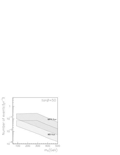
Figure 2: Theoretical predictions for the stau flux at IceCube as a function of the stau mass for different values of $\tan\beta$ in the CMSSM scenario with $A=0$.

In Fig. 2, we represent the stau flux as a function of stau mass for both WB and MPR neutrino fluxes and for $\tan\beta=10$ and $50$. Let us first examine the case $\tan\beta=10$. As expected, the production of heavier staus is suppressed, and therefore the flux decreases with the stau mass. We obtain, however, a band and not a line when we plot flux versus mass. This can be explained in the following way. Neutrino interactions leading to stau pair production involve the production of a squark, whose mass determines the energy threshold of the whole process. Squark masses are strongly dominated by gluino masses, which are roughly proportional to the common gaugino masses. Therefore, for the same value of the stau mass, the points on the $(m,M)$ plane corresponding to lower values of $M$ give rise to a lighter spectrum and thus lower energy thresholds. This, together with the $E^{-2}$ shape of the neutrino flux, implies a higher number of stau pairs for lower values of $M$. Turning to the figure, it is now easy to understand that, given a value for $m_{\widetilde{\tau}}$, the highest value of the flux corresponds to the lowest value of $M$ for which the stau is the LOSP. The lowest value, in turn, corresponds to the highest value of $M$, i.e., that corresponding to $m=0$. In the figure, the lower limit on the stau mass corresponds to the LEP experimental constraint on the Higgs (stau) mass for $\tan\beta=10$ (50).

For the $\tan\beta=50$ case, the flux is lower than that for $\tan\beta=10$ in approximately one order of magnitude. Notice that when $\tan\beta$ increases, the off-diagonal elements of the sparticle mass matrices become larger and the L-R mixing becomes more important. This implies a larger mass gap between the two mass eigenstates of the third family. Thus, for a fixed stau mass, the rest of the spectrum is heavier for $\tan\beta=50$ than for $\tan\beta=10$. This, according to the previous threshold energy argument, implies a lower flux. Notice finally that for $\tan\beta=50$ the experimental constraint on the branching ratio of the $b\to s\gamma$, which implies a lower bound on the common gaugino mass, leads to an upper bound on the predicted stau flux of about $0.2$ event yr^-1 for the MPR flux.

Thus the most optimistic results are obtained for light staus, and the lowest possible stau mass in the $\tan\beta=10$ scenario sets an upper limit to the predicted flux of about 1 event yr^-1 when the MPR flux is used (with the WB prediction this is reduced to $0.3$ event yr^-1). Notice that these results are smaller than those obtained in [3] due to the more constrained framework of supergravity analyses. Despite the fact that, as explained in the previous Section, the stau events can be distinguished from the dimuon background, these results evidence that, at best, several years of data from IceCube would be necessary to claim a positive signal. We will later see how this is modified when non-universal soft parameter are included.

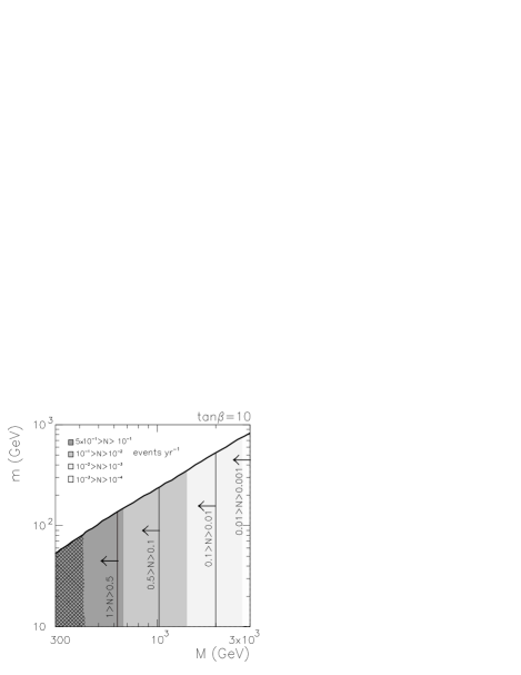
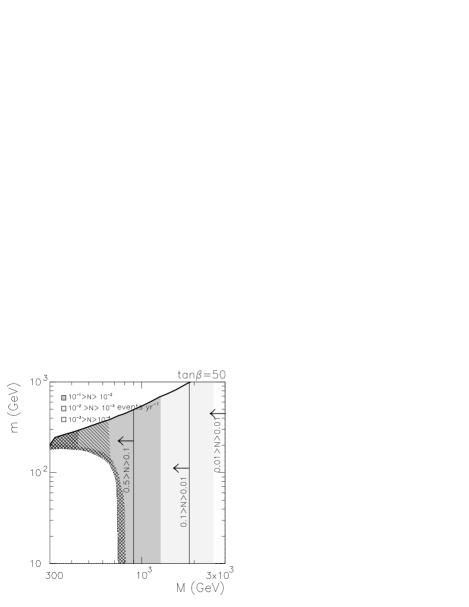
Figure 3: $(m,M)$ plane of the CMSSM scenario with $A=0$ and $\tan\beta=10,\,50$. The region below the thick solid line corresponds to that with stau LOSP. Coloured regions represent the theoretical predictions for the stau flux at IceCube in the case of WB neutrino flux, whereas vertical solid lines correspond to the results when the MPR flux is used. Gridded areas are experimentally excluded by LEP constraints on the Higgs and stau masses, whereas the ruled area is excluded by $b\rightarrow s\gamma$. The white area on the lower left corner of the plot for $\tan\beta=50$ is excluded due to the occurrence of negative stau squared-mass.

In order to understand which regions of the CMSSM parameter space could be explored using this technique, in Fig. 3 we superimpose the theoretical predictions for the stau flux on the $(m,M)$ plane for $A=0$ and $\tan\beta=10,\,50$. The most optimistic predictions regarding detectability occur for low values of $M$, corresponding to the regions with lighter staus and the flux decreases as the gaugino mass increases, with almost no dependence on the scalar mass parameter (when the stau mass is RG-evolved, the main contributions to it come from terms depending on gaugino masses). When the MPR prediction for the neutrino flux is used, a significant increase of the resulting stau flux is obtained.

To sort out the limits on the stau lifetime imposed by catalyzed BBN, the mass of the gravitino is constrained by an upper limit,

$$m_{\widetilde{G}}\leq 0.28\,\left(\frac{m_{\widetilde{\tau}}}{100\,\mathrm{GeV}}\right)^{5/2}\mathrm{GeV}\,,$$ (3.7)

which can be deduced from Eq.(3.5), setting the stau life equal to $5\times 10^{3}$ s. It can then be easily seen that the maximum gravitino mass ranges approximately from $0.2$ GeV to $20$ GeV, depending on the mass of the stau. For such light gravitinos, the relic density is fully dominated by thermal production,

$$\Omega^{TP}_{m_{\widetilde{G}}}\,h^{2}\approx 0.27\,\left(\frac{T_{R}}{10^{10}\,\mathrm{GeV}}\right)\left(\frac{100\,\mathrm{GeV}}{m_{\widetilde{G}}}\right)\left(\frac{m_{\widetilde{g}}(\mu)}{1\,\mathrm{TeV}}\right)^{2},$$ (3.8)

where $m_{\widetilde{g}}(\mu)$ is the running gluino mass [38, 39]. A relic density of about $0.1$, in agreement with WMAP data [40], can be recovered by an appropriate choice of the reheating temperature, depending on the mass of both the gravitino and the gluino. As $T_{R}\propto m_{\widetilde{G}}/m_{\widetilde{g}}^{2}$, we can make a rough estimation of the maximum value of $T_{R}$ as a function of the stau mass,

$$T_{R}\lesssim 5.2\times 10^{7}\left(\frac{m_{\widetilde{\tau}}}{100\,\mathrm{GeV}}\right)^{1/2}\mathrm{GeV}.$$ (3.9)

Similar upper bounds for the reheating temperature have been derived [33, 29, 41] and used to study its possible determination at the LHC [41]. It is finally worth pointing out that in this case the contribution to $\Omega_{DM}$ from non-thermal production is negligible.

As in the case of the gravitino, axino thermal production is a function of the reheating temperature [21, 42]. As emphasized in [43], the correct relic density can be obtained for nearly any point in the $(M,\,m)$ by fixing the axino mass and the reheating temperature. In particular, the regions with a small value of the gaugino mass (where the stau flux is maximal) could correspond to an axino with mass $m_{\widetilde{a}}\sim{{\cal O}(1\,{\rm GeV})}$ which must have a small reheating temperature, $T_{R}\sim 200\,{\rm GeV}$, in order to satisfy the constraint on its relic abundance. Notice that although a gauge invariant treatment of the axino thermal production [42] is only valid for larger $T_{R}$, this value can be obtained within the context of a quitessential kination scenario [44]. BBN constraints in this case are easily fulfilled since the stau lifetime is usually smaller than 1 second.

3.2 Neutralino LSP

Let us now consider a second interesting class of MSSM scenarios, those with a neutralino LSP as the dark matter candidate. Under these circumstances, in order to have a sufficiently long lifetime, the stau NLSP needs to be almost degenerate with the lightest neutralino. Interestingly, the quasi-degeneracy of the stau and lightest neutralino is also welcome from the point of view of neutralino dark matter. In such a situation the relic abundance of neutralinos is largely suppressed through a coannihilation mechanism [45], which makes it possible to find agreement with the constraints on the dark matter abundance [46]. Thus, this is another example in which supersymmetric scenarios which solve the dark matter problem can naturally provide long-lived staus.

The dependence of the stau lifetime on $\Delta m=m_{\widetilde{\tau}}-m_{\widetilde{\chi}^{0}}$ and on the left-right content of the mass eigenstate was studied in [47]. It was shown that in the regions where $\Delta m>m_{\tau}$, the 2-body decay $\widetilde{\tau}\rightarrow\tau\widetilde{\chi}^{0}$ is allowed, and it is the dominant process. In this case, the stau decays very rapidly, with a lifetime smaller or of the order of $10^{-17}$ s, and therefore never reaches the detector. On the other hand, if $\Delta m<m_{\tau}$, this channel closes, and typical lifetimes become $\mathcal{O}(10^{-6}\,\mathrm{s})$ or greater. This is long enough for staus to reach the detector before decaying .

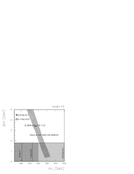
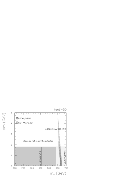
Figure 4: $(\Delta m,m_{\widetilde{\tau}})$ plane of the CMSSM scenario with $A=0$, $\tan\beta=10,50$ and neutralino LSP. Coloured regions represent the theoretical predictions for the stau flux at IceCube in the case of WB neutrino flux, whereas solid vertical lines correspond to the results when then MPR flux is used. Regions where WMAP relic density is reproduced are represented by gridded areas.

This is indeed a very restrictive requirement which only leaves a very narrow allowed band in the parameter space. In fact, such a small mass-difference between the neutralino LSP and the stau implies a too small relic density for the neutralino when its mass is small. The presence of staus with a sufficiently large lifetime is therefore only compatible with neutralino dark matter above a certain mass scale.

In order to illustrate this, we have represented in Fig. 4 the predicted flux of staus at the IceCube detector in the $(\Delta m,m_{\widetilde{\tau}})$ plane for an example of the CMSSM with $A=0$, $\mu>0$ and $\tan\beta=10,\,50$, and for both a WB and a MPR neutrino flux. As commented above, the flux vanishes for $\Delta m\raise 1.29167pt\hbox{$\;>$\kern-7.5pt\raise-4.73611pt\hbox{$\sim\;$}}2$ GeV. For $\Delta m\raise 1.29167pt\hbox{$\;<$\kern-7.5pt\raise-4.73611pt\hbox{$\sim\;$}}2$ GeV the flux increases as the stau mass decreases and can be as large as $2$ event yr^-1 for the MPR flux when the stau mass is close to its experimental lower bound. The WB flux is represented by means of a colour code, whereas the regions corresponding to different values of stau flux assuming a MPR neutrino flux are delimited by solid lines. The regions compatible with neutralino dark matter are represented on the same plane by means of gridded areas (for those points where the WMAP relic density is reproduced).

Compatibility of neutralino dark matter with observable staus is only possible for $\tan\beta=10$ and for $m_{\widetilde{\tau}}\approx 300$ GeV, thus implying a stau flux between $0.1$ and $0.5$ events yr^-1, in the optimistic MPR case or between $0.01$ and $0.1$ event yr^-1 if we work with a WB neutrino flux. For larger values of $\tan\beta$ the region where the neutralino relic density is compatible with WMAP results is shifted towards larger values of the stau mass and therefore is associated to much lower values of the stau flux. Once more, in spite of the good background discrimination, these small fluxes would require, at best, several years of data from IceCube.

3.3 General supergravity with non-universal soft terms

In the former Sections we have performed our calculations within the framework of the CMSSM. We will now briefly explore how the theoretical predictions for the stau flux vary when a more general supergravity scenario with non-universal soft parameters is considered. More specifically, we will try to identify possible non-universal schemes that lead to an increase of the theoretical predictions for the stau flux.

As we discussed above, the production rate of staus is very sensitive to the value of the squark masses, the resulting flux increasing in the presence of light squarks [1, 3]. Likewise, a decrease in the slepton masses is also welcome in order to increase their production cross-section. Moreover, as we can see in the Appendix, the expressions (A.12) corresponding to the chargino-mediated sfermion production are proportional to the factor $|Z_{+}^{1k}\ Z_{-}^{1k}|^{2}$. This implies that these contributions are enhanced when the lighter chargino is a pure wino state (i.e., $|Z_{+}^{1k}|\sim 1$).

A decrease of the low energy values for the squark masses, relative to the (right-handed) stau mass can be obtained if the ratio of the gluino and bino mass parameters, $M_{3}/M_{1}$, decreases at the GUT scale. The decrease in the squark masses induces a reduction of the $\mu$ parameter through the increase of the positive contributions to the RGE of $m_{H_{U}}^{2}$. This in turn implies an unwanted enhancement of the mixing in the chargino mass matrix. Thus, in order to compensate for the decrease in the $\mu$ parameter and have a pure wino as the lighter chargino, as well as reducing its mass, we must also decrease the $M_{2}$ parameter at the GUT scale. Smaller values of $M_{2}$ also imply a decrease in the masses for left-handed sleptons. Although, as mentioned above, this is also potentially good to increase their production cross-section, one should bear in mind that eventually the sneutrinos can become almost degenerate with the lighter stau and be long-lived. In that case left-handed squarks would generally cascade down to the lightest neutralino and this, in turn, mostly to sneutrinos which could propagate through the Earth without decaying into staus, thereby significantly attenuating the stau flux. We have avoided this situation by making sure sneutrinos decay promptly (with a lifetime smaller than $10^{-9}$ s), thus constraining the non-universality in $M_{2}$.

Finally, we can also attempt to increase the $\mu$ parameter, thus further enhancing the wino composition of the lightest chargino. This can be done by introducing a departure from universality in the Higgs mass parameters at the GUT scale. More specifically, we have considered an increase of the value of $m_{H_{U}}^{2}$ with respect to the mass of the rest of the scalars.

Figure 5: Supersymmetric spectrum corresponding to non-universal soft mass parameters as in Eq.(3.10) with $M=1000$ GeV, $m=20$ GeV, $A=0$ and $\tan\beta=10$.

As an specific example, following the above arguments we have taken the following set of non-universalities in the gaugino and scalar masses,

$$M_{2} = 0.6\,M_{1}\,$$

$$M_{3} = 0.5\,M_{1}\,$$

$$m_{H_{D},\,Q,\,U,\,D,\,L,\,E}^{2} = m^{2}\,,$$

$$m_{H_{U}}^{2} = 0.5\,m^{2}\,.$$ (3.10)

The resulting supersymmetric spectrum is depicted in Fig. 5 for $M=1000$ GeV and $m=20$ GeV, clearly evidencing the decrease in the masses of the squarks and heavy sleptons relative to the stau mass with respect to the universal case discussed in the previous Sections and shown in Fig. 1.

Given the change in the SUSY spectrum, we have redone the analysis of the decay chains that produce staus from squark and sleptons. We have checked that in this example the relation between the resulting stau energy and the parent squark and slepton reads

$$\langle E_{\widetilde{\tau}}\rangle\approx 0.8\,\langle E_{\widetilde{l}}\rangle\ ;\quad\quad\langle E_{\widetilde{\tau}}\rangle\approx 0.5\,\langle E_{\widetilde{q}}\rangle\ .$$ (3.11)

The increase in both quantities with respect to the universal case (see Eq.(3.6)) is due to the smaller mass differences among the supersymmetric particles which cascade to the lighter stau, which leads to a smaller suppression according to Eq.(A.14). These relations approximately hold throughout the whole region of the parameter space with stau LOSP.

Figure 6: The same as in Fig.2 but for the example with non-universal soft mass parameters as in Eq.(3.10).

The resulting theoretical predictions for the stau flux are represented in Fig. 6 as a function of the stau masses for both the WB and MPR flux for $A=0$ and $\tan\beta=10$. A moderate increase is observed with respect to the universal case of Fig. 2. For example, the results using the WB flux can reach now values of almost 1 event yr^-1, while those corresponding to the MPR flux are approximately a factor three larger.

4 Conclusions

We have explored the possibility of detecting long-lived staus at neutrino telescopes, after their production inside the Earth through the inelastic scattering of high energy neutrinos. More specifically, we have calculated the production rate of a pair of staus in terms of the high energy neutrino flux, evaluated their energy losses after traversing the distance to the experiment, and taken into account the track separation of the stau pair and the detector efficiency in order to compute the theoretical predictions for the resulting stau flux. We have studied two generic scenarios in which long-lived staus are naturally associated to a supersymmetric solution to the problem of dark matter.

On the one hand, we have considered the case of superWIMP dark matter in which the LSP is either the gravitino or the axino. Exploring the areas of the CMSSM in which the stau is the lightest observable particle we observed that the number of stau pairs is bounded to be below 1 event yr^-1 when the MPR neutrino flux is used. These predictions decrease by approximately a factor four for the WB flux. The largest values of the stau flux correspond to small values of $\tan\beta$ and to regions with a small value of the common gaugino mass. These areas of the parameter space can be consistent with viable gravitino dark matter for light gravitinos ($m_{\widetilde{G}}\raise 1.29167pt\hbox{$\;<$\kern-7.5pt\raise-4.73611pt\hbox{$\sim\;$}}1$ GeV), in order to avoid the stringent BBN constraints, or axinos with mass $m_{\widetilde{a}}\sim{{\cal O}(1\,{\rm GeV})}$ and a small reheating temperature, $T_{R}\sim 200\,{\rm GeV}$.

On the other hand, we have explored the case with a neutralino LSP. In this scenario, the stau can be long-lived if the mass difference with the neutralino is smaller than $\Delta m\raise 1.29167pt\hbox{$\;<$\kern-7.5pt\raise-4.73611pt\hbox{$\sim\;$}}2$ GeV. Interestingly, the neutralino-stau coannihilation region, where the WMAP relic density can be obtained, also occurs for small mass differences. We have studied this possibility within the CMSSM, finding that once more the largest results for the stau flux are obtained for small values of the gaugino mass parameter, i.e., for light staus, and increase when the rest of the spectrum (in particular the squark masses) is also light. This favours low values of $\tan\beta$. For $\tan\beta=10$, and using the MPR flux, an upper bound of approximately 2 events yr^-1 is found for staus with a mass of $m_{\widetilde{\tau}_{1}}\sim 100$ GeV, which decreases by a factor 2 for $\tan\beta=50$. When the WMAP constraint is imposed on the neutralino relic abundance, compatibility with viable neutralino dark matter reduces the allowed parameter space to a small range of stau masses. For example, with $\tan\beta=10$ one finds $m_{\widetilde{\tau}_{1}}\sim 300$ GeV, and the predicted stau flux is $0.1$ events yr^-1 . When $\tan\beta$ increases the region compatible is shifted to heavier staus and the resulting flux decreases significantly. Overall we have observed that the stau flux obtained in these supergravity scenarios is generally smaller than those of low energy supersymmetric analyses. This implies that, although stau events are distinguishable from the dimuon backround, in the most optimistic scenarios several years of data from IceCube are necessary to claim a positive signal.

Finally, we have investigated the case of a general supergravity theory in which the structure of the soft parameters is non-universal. We have observed that certain choices of non-universalities which lead to wino-like charginos and a decrease of the squark and slepton masses can account for a moderate increase of the resulting stau flux. More specifically, through a decrease of both the gluino and wino mass parameters with respect to the bino mass and a decrease of the soft mass for the $H_{u}$ Higgs at the GUT scale we have shown that the stau flux can increase by approximately a factor three with respect to the results in the CMSSM.

Acknowledgements

We thank K.Y. Choi and P. Slavich for very useful discussions. This work was supported in part by the Spanish DGI of the MEC under Proyecto Nacional FPA2006-01105, by the Comunidad de Madrid under Proyecto HEPHACOS, Ayudas de I+D S-0505/ESP-0346, by the EU RTN UniverseNet MRTN-CT-2006-035863, and by the ENTApP Network of the ILIAS project RII3-CT-2004-506222. The work of B. Cañadas has been partially supported by an INFN-Roma Tor Vergata FAI grant for foreign researchers and thanks the INFN-Roma Tor Vergata for their kind hospitality during the last stages of this work. D.G. Cerdeño is supported by the program “Juan de la Cierva” of the Ministerio de Educación y Ciencia of Spain. The work of C. Muñoz was supported in part by the Spanish DGI of the MEC under Proyecto Nacional FPA2006-05423, and by the EU under the RTN program MRTN-CT-2004-503369.

Appendix A Sfermion production from neutrino inelastic scattering

The contribution from chargino exchange along a $t$-channel comprises the diagrams shown in the upper row in Fig. 7. They lead to the following cross-sections,

$$\frac{d\sigma}{dt}\Big{|}_{\nu d}= \frac{\pi\alpha^{2}}{2s_{W}^{4}}\frac{1}{s}\left[\frac{m_{\widetilde{\chi}^{+}_{k}}|Z_{U}^{Ii}||Z_{L}^{Jj}||Z_{+}^{1k}||Z_{-}^{1k}|}{t-m_{\widetilde{\chi}^{+}_{k}}^{2}}\right]^{2},$$

$$\frac{d\sigma}{dt}\Big{|}_{\nu\bar{u}}= \frac{\pi\alpha^{2}}{2s_{W}^{4}}\frac{1}{s^{2}}\left[\frac{Z_{-}^{1k}Z_{-}^{1k}}{t-m_{\widetilde{\chi}^{+}_{k}}^{2}}\right]^{2}|Z_{D}^{Ii}||Z_{L}^{Jj}|\left(tu-m_{\widetilde{d}_{i}}^{2}m_{\widetilde{l}_{j}}^{2}\right)\ ,$$ (A.12)

with notation for $Z$ matrices in agreement with that of [48], where $Z_{+}$ and $Z_{-}$ are $2\times 2$ chargino mixing matrices, with $k=1,2$, and $Z_{U}$, $Z_{D}$ and $Z_{L}$ are $6\times 6$ squark mixing matrices. Capital indices $I$ and $J$ are family indices running from 1 to 3, whereas indices $i$ and $j$ stand for mass eigenstates and run from 1 to 6. Summation over all indices is implied.

For the diagrams with neutralino exchange along a $t$-channel, shown on the lower row of Fig. 7, we make the following definitions,

$$\begin{array}[]{ll}{N}_{i}^{\nu_{L}}=c_{W}Z_{N}^{2i}-s_{W}Z_{N}^{1i}\,,&\cr{N}_{i}^{u_{L}}=c_{W}Z_{N}^{2i}+\frac{1}{3}s_{W}Z_{N}^{1i}\,,&{N}_{i}^{u_{R}}=\frac{4}{3}s_{W}Z_{N}^{1i}\,,\cr{N}_{i}^{d_{L}}=-c_{W}Z_{N}^{2i}+\frac{1}{3}s_{W}Z_{N}^{1i}\,,&{N}_{i}^{d_{R}}=-\,\frac{2}{3}s_{W}Z_{N}^{1i}\,.\end{array}$$

The total cross-section for interaction with quarks, expressed in terms of mass eigenstates, reads

$$\frac{d\sigma}{dt}\Big{|}_{\nu q}=\frac{\pi\alpha^{2}}{8s_{W}^{4}c_{W}^{4}}\frac{1}{s^{2}}\left\{s\left[\frac{m_{\widetilde{\chi}^{0}_{k}}{N}_{k}^{q_{L}}{N}_{i}^{\nu_{L}}|Z_{U/D}^{Ii}|}{(t-m_{\widetilde{\chi}^{0}_{k}}^{2})}\right]^{2}+\sum_{i}\left[\frac{{N}_{i}^{q_{R}}{N}_{i}^{\nu_{L}}|Z_{U/D}^{(I+3)i}|}{(t-m_{\widetilde{\chi}^{0}_{i}}^{2})}\right]^{2}(tu-m_{\widetilde{q_{i}}}^{2}m_{\widetilde{\nu}}^{2})\right\}\,,$$

$$\frac{d\sigma}{dt}\Big{|}_{\nu\bar{q}}=\frac{\pi\alpha^{2}}{8s_{W}^{4}c_{w}^{4}}\frac{1}{s^{2}}\left\{s\left[\frac{m_{\widetilde{\chi}_{i}^{0}}^{2}{N}_{i}^{u_{R}/d_{R}}{N}_{i}^{\nu_{L}}|Z_{U/D}^{(I+3)i}|}{(t-m_{\widetilde{\chi}^{0}_{i}}^{2})}\right]^{2}+\left[\frac{{N}_{i}^{u_{L}/d_{L}}{N}_{i}^{\nu_{L}}|Z_{U/D}^{Ii}|}{(t-m_{\widetilde{\chi}^{0}_{i}}^{2})}\right]^{2}(tu-m_{\widetilde{q}^{2}\widetilde{l}^{2}})\right\}$$ (A.13)

These parton-level cross-sections are then convoluted with their corresponding Parton Distribution Functions, which we extract from the Cteq6PDF package [36].

Figure 7: Feynman diagrams describing the different neutrino inelastic interactions.

To calculate the fraction of the parent’s energy carried by the stau, we use the general formula

$$E_{\widetilde{\tau}}^{LAB}=\frac{E_{parent}^{LAB}}{2^{n}}\prod_{i=1,n}\left(1+\frac{m_{i}^{2}}{m_{i-1}^{2}}\right)\ ,$$ (A.14)

where $n$ is the number of intermediate states, $i=0$ corresponds to the parent squark or slepton, and $i=n$ corresponds to the stau.

References

- [1] I. Albuquerque, G. Burdman and Z. Chacko, Phys. Rev. Lett. 92 (2004) 221802 [arXiv:hep-ph/0312197].
- [2] M. Ahlers, J. Kersten and A. Ringwald, JCAP 07 (2006) 005 [arXiv:hep-ph/0604188].
- [3] I. F. M. Albuquerque, G. Burdman and Z. Chacko, Phys. Rev. D 75 (2007) 035006 [arXiv:hep-ph/0605120].
- [4] M. Ahlers, J. Phys. Conf. Ser. 60 (2007) 171 [arXiv:astro-ph/0610775].
- [5] I. F. M. Albuquerque, G. Burdman, C. A. Krenke and B. Nosratpour, Phys. Rev. D 78 (2008) 015010 [arXiv:0803.3479 [hep-ph]].
- [6] M. Ahlers, J. I. Illana, M. Masip and D. Meloni, JCAP 0708 (2007) 008 [arXiv:0705.3782 [hep-ph]].
- [7] S. Ando, J. F. Beacom, S. Profumo and D. Rainwater, JCAP 04 (2008) 029 [arXiv:0711.2908 [hep-ph]].
- [8] H. Goldberg, Phys. Rev. Lett. 50 (1983) 1419; J. R. Ellis, J. S. Hagelin, D. V. Nanopoulos and M. Srednicki, Phys. Lett. B 127 (1983) 233 ; L. M. Krauss, Phys. Lett. B 128 (1983) 37 ; J. R. Ellis, J. S. Hagelin, D. V. Nanopoulos, K. A. Olive and M. Srednicki, Nucl. Phys. B 238 (1984) 453.
- [9] H. Pagels and J. R. Primack, Phys. Rev. Lett. 48 (1982) 223; S. Weinberg, Phys. Rev. Lett. 48 (1982) 1303.
- [10] K. Rajagopal, M. S. Turner and F. Wilczek, Nucl. Phys. B 358 (1991) 447; E. J. Chun, J. E. Kim and H. P. Nilles, Phys. Lett. B 287 (1992) 123 [arXiv:hep-ph/9205229].
- [11] E. Waxman and J. N. Bahcall, Phys. Rev. D 59 (1999) 023002 [arXiv:hep-ph/9807282]; J. N. Bahcall and E. Waxman, Phys. Rev. D 64 (2001) 023002 [arXiv:hep-ph/9902383].
- [12] K. Mannheim, R. J. Protheroe and J. P. Rachen, Phys. Rev. D 63 (2001) 023003 [arXiv:astro-ph/9812398].
- [13] [IceCube Collaboration], arXiv:0711.0353 [astro-ph].
- [14] R. Gandhi, C. Quigg, M. H. Reno and I. Sarcevic, Astropart. Phys. 5 (1996) 81 [arXiv:hep-ph/9512364].
- [15] M. H. Reno, I. Sarcevic and S. Su, Astropart. Phys. 24 (2005) 107 [arXiv:hep-ph/0503030].
- [16] Y. Huang, M. H. Reno, I. Sarcevic and J. Uscinski, Phys. Rev. D 74 (2006) 115009 [arXiv:hep-ph/0607216].
- [17] J. Ahrens et al. [IceCube Collaboration], Astropart. Phys. 20 (2004) 507 [arXiv:astro-ph/0305196].
- [18] E. Barberio et al. [Heavy Flavor Averaging Group (HFAG) Collaboration], “Averages of b-hadron properties at the end of 2006,” arXiv:0704.3575 [hep-ex].
- [19] M. Misiak and M. Steinhauser, ‘NNLO QCD corrections to the matrix elements using interpolation in ’, Nucl. Phys. B 764 (2007) 62 [arXiv:hep-ph/0609241]; M. Misiak et al., ‘The first estimate of B at ’, Phys. Rev. Lett. 98 (2007) 022002 [arXiv:hep-ph/0609232].
- [20] J. L. Feng, A. Rajaraman and F. Takayama, Phys. Rev. Lett. 91 (2003) 011302 [arXiv:hep-ph/0302215]; J. L. Feng, A. Rajaraman and F. Takayama, Phys. Rev. D 68 (2003) 063504 [arXiv:hep-ph/0306024]; J. L. Feng, S. Su and F. Takayama, Phys. Rev. D 70 (2004) 075019 [arXiv:hep-ph/0404231]. K. Y. Choi and L. Roszkowski, AIP Conf. Proc. 805 (2006) 30 [arXiv:hep-ph/0511003].
- [21] L. Covi, J. E. Kim and L. Roszkowski, Phys. Rev. Lett. 82 (1999) 4180 [arXiv:hep-ph/9905212]; L. Covi, H. B. Kim, J. E. Kim and L. Roszkowski, JHEP 0105 (2001) 033 [arXiv:hep-ph/0101009].
- [22] M. Fujii, M. Ibe and T. Yanagida, Phys. Lett. B 579 (2004) 6 [arXiv:hep-ph/0310142].
- [23] L. Roszkowski, R. Ruiz de Austri and K. Y. Choi, JHEP 08 (2005) 080 [arXiv:hep-ph/0408227].
- [24] R. H. Cyburt, J. R. Ellis, B. D. Fields and K. A. Olive, Phys. Rev. D 67 (2003) 103521 [arXiv:astro-ph/0211258]. M. Kawasaki, K. Kohri and T. Moroi, Phys. Lett. B 625 (2005) 7 [arXiv:astro-ph/0402490]; M. Kawasaki, K. Kohri and T. Moroi, Phys. Rev. D 71 (2005) 083502 [arXiv:astro-ph/0408426];
- [25] W. Hu and J. Silk, Phys. Rev. Lett. 70 (1993) 2661.
- [26] J. R. Ellis, J. E. Kim and D. V. Nanopoulos, Phys. Lett. B 145 (1984) 181.
- [27] K. Hagiwara et al. [Particle Data Group], Phys. Rev. D 66 (2002) 010001.
- [28] M. Pospelov, Phys. Rev. Lett. 98 (2007) 231301 [arXiv:hep-ph/0605215].
- [29] J. Pradler and F. D. Steffen, Phys. Lett. B 666 (2008) 181 [arXiv:0710.2213 [hep-ph]].
- [30] M. Pospelov, J. Pradler and F. D. Steffen, JCAP 0811 (2008) 020 [arXiv:0807.4287 [hep-ph]].
- [31] J. R. Ellis, K. A. Olive, Y. Santoso and V. C. Spanos, Phys. Lett. B 588 (2004) 7 [arXiv:hep-ph/0312262].
- [32] D. G. Cerdeño, K. Y. Choi, K. Jedamzik, L. Roszkowski and R. Ruiz de Austri, JCAP 06 (2006) 005 [arXiv:hep-ph/0509275].
- [33] J. Pradler and F. D. Steffen, Phys. Lett. B 648 (2007) 224 [arXiv:hep-ph/0612291].
- [34] J. L. Feng, S. Su and F. Takayama, Phys. Rev. D 70 (2004) 075019 [arXiv:hep-ph/0404231].
- [35] F. E. Paige, S. D. Protopopescu, H. Baer and X. Tata, arXiv:hep-ph/0312045.
- [36] J. Pumplin, D. R. Stump, J. Huston, H. L. Lai, P. Nadolsky and W. K. Tung, JHEP 07 (2002) 012 [arXiv:hep-ph/0201195]. J. Pumplin, A. Belyaev, J. Huston, D. Stump and W. K. Tung, JHEP 02 (2006) 032 [arXiv:hep-ph/0512167].
- [37] A. D. Martin, W. J. Stirling and R. S. Thorne, Phys. Lett. B 636 (2006) 259 [arXiv:hep-ph/0603143].
- [38] M. Bolz, A. Brandenburg and W. Buchmuller, Nucl. Phys. B 606 (2001) 518 [Erratum-ibid. B 790 (2008) 336] [arXiv:hep-ph/0012052].
- [39] J. Pradler and F. D. Steffen, Phys. Rev. D 75 (2007) 023509 [arXiv:hep-ph/0608344].
- [40] M. R. Nolta et al. [WMAP Collaboration], arXiv:0803.0593 [astro-ph].
- [41] K. Y. Choi, L. Roszkowski and R. Ruiz de Austri, JHEP 04 (2008) 016 [arXiv:0710.3349 [hep-ph]]; F. D. Steffen, Phys. Lett. B 669 (2008) 74 [arXiv:0806.3266 [hep-ph]].
- [42] A. Brandenburg and F. D. Steffen, JCAP 0408 (2004) 008 [arXiv:hep-ph/0405158].
- [43] L. Covi, L. Roszkowski, R. Ruiz de Austri and M. Small, JHEP 06 (2004) 003 [arXiv:hep-ph/0402240].
- [44] M. E. Gomez, S. Lola, C. Pallis and J. Rodriguez-Quintero, arXiv:0809.1859 [hep-ph].
- [45] K. Griest and D. Seckel, Phys. Rev. D 43 (1991) 3191.
- [46] J. R. Ellis, T. Falk and K. A. Olive, Phys. Lett. B 444 (1998) 367 [arXiv:hep-ph/9810360].
- [47] T. Jittoh, J. Sato, T. Shimomura and M. Yamanaka, Phys. Rev. D 73 (2006) 055009 [arXiv:hep-ph/0512197].
- [48] J. Rosiek, arXiv:hep-ph/9511250.