The Coyote Universe I: Precision Determination of the Nonlinear Matter Power Spectrum

Abstract

Near-future cosmological observations targeted at investigations of dark energy pose stringent requirements on the accuracy of theoretical predictions for the nonlinear clustering of matter. Currently, $N$-body simulations comprise the only viable approach to this problem. In this paper we study various sources of computational error and methods to control them. By applying our methodology to a large suite of cosmological simulations we show that results for the (gravity-only) nonlinear matter power spectrum can be obtained at 1% accuracy out to $k\sim 1\,h\,{\rm Mpc}^{-1}$. The key components of these high accuracy simulations are: precise initial conditions, very large simulation volumes, sufficient mass resolution, and accurate time stepping. This paper is the first in a series of three; the final aim is a high-accuracy prediction scheme for the nonlinear matter power spectrum that improves current fitting formulae by an order of magnitude.

                                                                                                                                     LA-UR-08-05630

1 Introduction

The nature of the dark energy believed to be causing the current accelerated expansion of the Universe is one of the greatest puzzles in the physical sciences, with deep implications for our understanding of the Universe and fundamental physics. The twin aims of better characterizing and further understanding the nature of dark energy are widely recognized as key science goals for the next decade. Although dark energy remains very poorly understood, theory nevertheless plays an essential role in furthering this enterprise.

The phenomenology of cosmological models is theory-driven not only in terms of providing explanations for the diverse phenomena that are observed, as well as promoting alternative explanations of existing measurements, but also due to the increasing reliance on theorists to produce sophisticated numerical models of the Universe which can be used to refine and calibrate experimental probes. Without a dedicated effort to develop the tools and skill-sets necessary for the interpretation of the next generation of experiments, we risk being “theory limited” in essentially all areas of dark energy studies.

As a concrete example of this general trend, forecasts for determination of the dark energy equation of state and other cosmological parameters from next-generation observations of cosmological structure typically assume calibration against simulations accurate to the level of 1% or better. This target has rarely been met for simulations of complex nonlinear phenomena such as the formation of large-scale structure in the Universe. However it is precisely these probes, which provide information on both the geometry of space-time and the growth of large-scale structure, which will be key to unraveling the mystery of dark energy.

For upcoming measurements to be exploited to the full, theory must reach not only the levels of accuracy justified by the measurements but also cover a sufficiently wide range of cosmologies. The problem breaks down to two questions: (i) What is a reasonable coverage of cosmological parameters, given the expected set of observations? (ii) What is the required accuracy for theoretical predictions – over this range of parameters – for the given set of observations? It is crucial to realize that the ultimate requirement is on controlling the absolute error – taking into account all of the relevant physics: gravity, hydrodynamics, and feedback mechanisms. This is much more difficult to achieve than relative error control – e.g. asking what the relative importance of baryonic physics is versus a baseline gravity-only simulation. Most recent papers discuss the latter, implicitly assuming the existence of a reference spectrum. One aim of our work is to provide just such a reference spectrum within the boundaries outlined. We fully expect that the answers to both (i) and (ii) will evolve, requiring more accurate modeling of a smaller range of models, so we are most interested here in the near-term needs. Associated with the first problem is the fact that, given the impossibility of running complex simulations over the many thousands of cosmologies necessary for grid based or Markov Chain Monte Carlo (MCMC) estimation of cosmological parameters, one must develop efficient interpolation methods for theoretical predictions. These methods must of course also satisfy the accuracy requirements of question (ii).

The control of errors in the underlying theory for the CMB is adequate to analyze results from Planck (Seljak et al., 2003; Wong et al., 2008). This is, however, not the case for predictions of gravitational clustering in the nonlinear regime, as is required for cluster counts, redshift space distortions, baryon acoustic oscillations (BAO) and weak lensing (WL) observations. In the case of BAO, the galaxy power spectrum in the quasi-linear regime should be known to sub-percent accuracy, and for WL the same is true for the mass power spectrum to significantly smaller scales. Perturbation theory has errors on the mass power spectrum currently estimated to be at the percent level in the weakly nonlinear regime (see, e.g., Jeong & Komatsu 2006 and Carlson et al. 2009 for recent treatments, or Bernardeau et al. 2002 for an earlier review). To reduce these errors, test the approximations, and model galaxy bias, numerical simulations are unavoidable. Theoretical templates, in terms of current power spectrum fits based on simulations (with errors at the 5% level), are already a limiting factor for WL observations at wavenumbers $k\sim 1\,h\,{\rm Mpc}^{-1}$. Huterer & Takada (2005) show that in order to avoid errors from imprecise theoretical templates mimicking the effect of cosmological parameter variations, the power spectrum has to be calibrated at about 0.5-1% for $0.1\,h\,{\rm Mpc}^{-1}\leq k\leq 10\,h\,{\rm Mpc}^{-1}$. The scale most sensitive for WL measurements is around $k\sim 1\,h\,$Mpc^-1 and $z\sim 0.5$ and the power spectrum therefore needs to be calibrated the most accurately at that point (see, e.g, Huterer & Takada 2005, Figure 1). In a very recent paper, Hilbert et al. (2008) re-emphasize the need for very accurate predictions for the theoretical power spectrum, pointing out that currently used fitting functions such as the Peacock & Dodds (1996) formula or the fit derived by Smith et al. (2003) underestimate the cosmic shear-power spectra by $>30\%$ for $k>10\,h\,{\rm Mpc}^{-1}$.

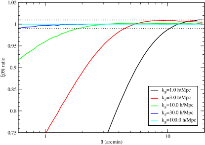
Figure 1: Ratio of the E-mode correlation function with and without an assumed suppression of the power spectrum mimicking a possible systematic error in the matter power spectrum. This figure demonstrates that a gradual decrease in the accuracy of the matter power spectrum on small scales will not lead to a catastrophic error in the weak lensing prediction. The green line with $k_{F}=10\,h\,{\rm Mpc}^{-1}$ corresponds to error properties which will be close to the degradation we expect for the matter power spectrum presented in this paper (see text).

We have independently assessed the impact a mis-modeled power spectrum would have on the predictions of weak lensing observables, including the fact that a wide range of spatial scales can be mapped into a given angular scale. Assuming a distribution of sources with $\langle z\rangle=1$, and using the Limber approximation, we compute the observable shear-shear correlation function, $\xi(\theta)=\langle\gamma(0)\cdot\gamma(\theta)\rangle$, given an estimate of the $z$-dependent mass power spectrum, $\Delta^{2}(k,z)$. To mimic the inaccuracy of $\Delta^{2}(k,z)$ on scales smaller than $1\,h\,{\rm Mpc}^{-1}$, we multiply it by a $z$-independent filter of the form $(1+k^{2}/k_{F}^{2})^{-1}$ for a variety of $k_{F}$. At $\ell=1000$ the suppression is 2-3% for $k_{F}=1\,0\,h\,{\rm Mpc}$ ($k_{F}$ being the assumed suppression of the power spectrum) and it drops to 1% at $\ell~{}500$. Assuming that $k_{F}\simeq 10\,h\,{\rm Mpc}^{-1}$ reflects the error properties we are aiming at in this paper (i.e. $\Delta^{2}\sim 1\%$ low at $k\simeq\,1\,h\,$Mpc^-1 and smoothly but increasingly low for smaller scales) we expect our results could be used to predict the shear correlation function at the percent level for separations larger than $2^{\prime}$. Figure 1 shows the expected error for different filter scales. Assuming sources at higher $z$ shifts all of the curves to larger scales, while a lower source redshift shifts the curves to smaller scales.

In order to extract precise cosmological information from WL measurements, additional physics beyond the gravitational contribution must be taken into account. At length scales smaller than $k\sim 1\,h\,{\rm Mpc}^{-1}$, baryonic effects are expected to be larger than 1% (White, 2004; Zhan & Knox, 2004; Jing et al., 2006; Rudd et al., 2008; Guillet, Teyssier & Colombi, 2009) and will have to be treated separately, either directly via hydrodynamic simulations or, as is more likely, by a combination of simulations and self-calibration techniques (e.g. constraining cluster profiles by cluster-galaxy lensing at the same time as constraining the shear). In any case, gravitational $N$-body simulations must remain the bedrock on which all of these techniques are based.

Taking all of these considerations into account, the purpose of this paper is to establish that gravitational $N$-body simulations can produce power spectra accurate to 1% out to $k\sim 1\,h\,{\rm Mpc}^{-1}$ between $z=0-1$ for a range of cosmological models. Given the success of the CDM paradigm in explaining current observational data we shall consider cosmologies within that framework. All of our models will assume a spatially flat Universe with purely adiabatic fluctuations and a power-law power spectrum. Since it is unlikely that near-term observations can place meaningful constraints on the temporal variation of the equation of state of the dark energy, we will restrict attention to cosmologies with a constant equation of state parameter $w=-p/\rho$ (where $p$ is the pressure and $\rho$ the density of the dark energy with $w=-1$ in a $\Lambda$CDM cosmology). Since $\Lambda$CDM is a good fit to the data, the accuracy of simulations can be established primarily around this point.

In this paper we will establish that gravitational $N$-body simulations can meet the above demands and derive a set of simulation criteria which balance the need for accuracy against computational costs. The target regime covers the most important range for current and near-future WL surveys and additional physics is controllable at the required level of accuracy. Showing that the required accuracy can be obtained from $N$-body simulations is only the first step in setting up a power spectrum determination scheme useful for weak lensing surveys. In order to analyze observational data and infer cosmological parameters, precise predictions for the power spectrum over a large range of cosmologies are required. This paper – establishing that achieving the base accuracy is possible – is the first in a series of three communications. In the second, we will demonstrate that a relatively small number of numerically obtained power spectra are sufficient to derive an accurate prediction scheme – or emulator – for the power spectrum covering the full range of desired cosmologies. The third paper of the series will present results from the complete simulation suite, named the “Coyote Universe” after the computing cluster on which it has been carried out. The third paper will also contain a public release of a precision power spectrum emulator.

In order to establish the accuracy over the required spatial dynamic range, as well as over the redshifts probed, a variety of tests need to be conducted. These include studies of the initial conditions, convergence to linear theory at very large length scales, the mass resolution requirement, and other evolution-specific requirements such as force resolution and time-stepping errors. To establish robustness of the final results, codes based on different $N$-body algorithms should independently converge to the same results (within error bounds). While some of these studies have been conducted separately and within the confines of the cosmic code verification project Heitmann et al. (2007), this is the first time that the more or less complete set of possible problems has been investigated in realistic simulations.

We find that it is indeed possible to control the accuracy of $N$-body simulations at 1% out to $k\sim 1\,h\,{\rm Mpc}^{-1}$. Even though these scales are not very small, the simulation requirements are rather demanding. First, the simulation volume needs to be large enough to capture the linear regime accurately. Due to mode-mode coupling, nonlinear effects influence scales as large as 500 $h^{-1}$Mpc. Therefore, the simulation volume needs to cover at least 1 ($h^{-1}$Gpc)³. Second, with this requirement imposed, the number of particles necessary to avoid errors from discreteness effects at the smallest length scales of interest, also becomes substantial. As we discuss later, because we are measuring the mass power spectrum (which is sensitive to near-mean-density regions) numerical results aiming for accuracy at the sub-percent level can only be trusted at scales below the particle Nyquist wavenumber (see also Joyce et al., 2008). A $1\,(h^{-1}{\rm Gpc})^{3}$ simulation volume requires a minimum particle loading of a billion particles. Third, it is important to start the simulation at a high enough redshift to allow enough dynamic range (in time) for structures to evolve correctly and for the initial perturbations to be captured accurately by the Zel’dovich approximation (ZA). Lastly, the force resolution and time stepping has to be accurate enough to ensure convergence of the simulation results.

The paper is organized as follows. In Section 2 we use a simple example to demonstrate the need for precision predictions from theory. Section 3 contains a description of the $N$-body codes used in this paper and some basic information about the simulations. In Section 4 we briefly describe the power spectrum estimator. In Sections 5 and 6 investigations of initial conditions and time evolution are reported, demonstrating that the simulations can achieve the required accuracy levels. Finally, we compare the numerical results to the commonly used semi-analytic HaloFit approach (Smith et al., 2003) in Section 7, finding a discrepancy of $\sim 5-10\%$ between the fit and the simulations. We provide a summary discussion of our results in Section 8. Appendix A discusses errors in setting up the initial conditions, comparing the Zel’dovich and 2LPT approximations. Appendix B provides details of the Richardson extrapolation procedure used for some of the convergence tests.

2 The Precision Cosmology Challenge

Before discussing how to achieve 1% accuracy for the nonlinear power spectrum, we will briefly demonstrate the importance of accurately determining the power spectrum. In our example, we assume the ability to measure the power spectrum from observations at $1\%$ accuracy in the quasi-linear and nonlinear regimes. On larger scales, accounting for sample variance (statistical limitations due to finite volume-sampling) leads to an increase in the statistical error, of up to 10%. These values are rough estimates, which are sufficient to make our point in this simple example.

For our example, we use a halo model-inspired fitting formula given by the code HaloFit as implemented in CAMB. Under the assumptions going into HaloFit it can be straightforwardly modified for $w$CDM cosmologies by simply adjusting the linear power spectrum and the linear growth function to account for $w\not=-1$ (explicit tests for some cosmologies were presented in Ma 2007). Current weak lensing analyses (see, e.g., Kilbinger et al. 2008) rely on HaloFit to derive constraints for $w$CDM cosmologies due to the lack of a better alternative. HaloFit is therefore the natural choice for our example.

We generate two sets of mock measurements: one from a power spectrum generated with HaloFit and another directly from a set of high-precision simulations. We then move points off the base power spectrum according to a Gaussian distribution with variance specified by the error estimates given above. The resulting mock data points and the underlying power spectra are shown in Figure 2. On a logarithmic scale, the data points and power spectra are almost indistinguishable. As we will show later in Section 7, the difference between the HaloFit and $N$-body power spectra is at the 5-10% level: this difference is enough to lead to significant biases in parameter estimation.

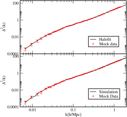
Figure 2: Upper panel: Synthetic data from a HaloFit run. Lower panel: Synthetic data from a combination of several $N$-body runs. In both cases the black line shows the underlying power spectrum from which the data was drawn and the red points show 34 data points with error bars. At small spatial scales, the assumed error is 1%, rising to 10% at large scales due to increased sample variance.

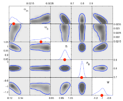
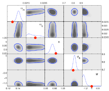
Figure 3: Posterior distributions for the five parameters under consideration. Upper panel: Results for the analysis of the HaloFit synthetic data set analyzed with a set of HaloFit power spectra. The red dots indicate the true values. As is to be expected, the constraints on the parameters are very good. Lower panel: Results for the HaloFit-based analysis of the $N$-body synthetic data set. Note that the constraints for $\omega_{m}$ and $w$ are now incorrect at $\sim 20$%.

We determine the best-fit parameters from the two mock data sets using the following parameter priors:

$$0.02\leq \omega_{b} \leq 0.025,$$

$$0.11\leq \omega_{m} \leq 0.15,$$

$$0.85\leq n_{s} \leq 1.05,$$

$$-1.3\leq w \leq-0.7,$$

$$0.7\leq \sigma_{8} \leq 0.9,$$ (1)

where $\omega_{b}=\Omega_{b}h^{2}$ and $\omega_{m}=\Omega_{m}h^{2}$. We do not treat $h$ as an independent variable but determine it via the CMB constraint $l_{A}=\pi d_{lss}/r_{s}=302.4$ where $d_{lss}$ is the distance to the last scattering surface and $r_{s}$ is the sound horizon (more details of how we construct our model sampling space are provided in Heitmann et al. 2009, Paper II).

The parameter estimation analysis then proceeds via a combination of model interpolation and Markov Chain Monte Carlo (MCMC) as implemented in our recently introduced cosmic calibration framework (Habib et al., 2007). We use HaloFit to generate the nonlinear power spectra for the MCMC analysis. That is, we analyze a HaloFit synthetic data set and one generated from numerical simulations against a set of model predictions from HaloFit generated power spectra. The results, which are all obtained from data at $z=0$, are shown in Figure 3. The upper panel shows the results from the analysis of the HaloFit synthetic data, where the parameter estimation works extremely well, being essentially a consistency check for the statistical framework. The result also points to the constraining power of matter power spectrum data. The lower panel in Figure 3 shows the corresponding result for the synthetic data generated directly from the simulations. In this case, the $\sim 5\%$ errors in the HaloFit model predictions are clearly seen to be problematic: most of the parameters are significantly off, $\omega_{m}$ and $w$ being mis-estimated by $\sim 20$%.

The example used here is certainly too simplified, relying only on large scale structure “observations” and making no attempt to take into account covariance, degeneracies, other observations, etc. For example, including a second observational probe such as the cosmic microwave background would provide a tighter constraint on $\sigma_{8}$, reducing the 20% shift in $w$. Nevertheless, the example clearly illustrates the general point that to perform an unbiased data analysis the theory underlying the analysis framework must match or preferably exceed the accuracy of the data.

3 $N$-body codes and Simulations

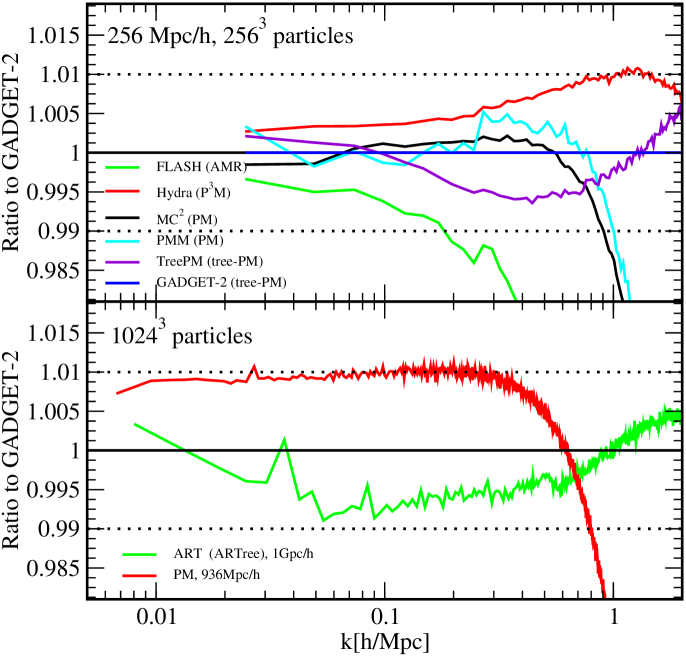
Figure 4: Upper panel: Comparison of dimensionless power spectra from a handful of $N$-body codes, taken from the data of Heitmann et al. (2007) for the “LCDMb” box: a $\Lambda$CDM model with $\Omega_{m}=0.314$, $h=0.71$, $n_{s}=0.99$, and $L_{\rm box}=256\,h^{-1}$Mpc with 256³ particles. The two PM codes, MC² and PMM, were run on a 1024³ grid (with a grid-to-particle ratio of 4:1, a factor of two higher than used for the PM runs in this paper). The FLASH run had a base grid of 256³ and a refinement level of two. Therefore, the force resolution of the purely grid-based codes is roughly a factor of ten lower than for the other codes (the different force kernels make a precise comparison difficult). The dotted lines show the 1% agreement limit. The high force-resolution codes agree to ${\mathcal{O}}(1\%)$ up to $k\sim 1\,h\,{\rm Mpc}^{-1}$ despite different choices for the force softening and other numerical parameters. Lower panel: Comparison of GADGET-2 and ART for a simulation with 1024³ particles and $L_{\rm box}=1~{}h^{-1}$Gpc. The cosmological parameters are very close to those for our major runs, the main difference being the starting redshift of $z_{\rm in}=65.66$. The agreement of the two codes is better than 1% over all scales. In addition, we compare one of the PM runs used in this paper with respect to GADGET-2. The agreement is also at ${\mathcal{O}}(1\%)$. We re-emphasize that our goal is to derive simulation requirements for percent level accuracy and finding a good balance between efficient computing and accuracy. By tuning code parameters, the agreement between different codes may be improved, but this would defeat the purpose of testing for robustness.

The numerical computations carried out and analyzed in this paper are $N$-body simulations that model structure formation in an expanding universe assuming that gravity dominates all other forces. The phase space density field is sampled by finite-mass particles and these particles are evolved using self-consistent force evaluations. Although the effects of baryons and neutrinos are taken into account while setting up initial conditions, only their gravitational contribution to the ensuing nonlinear dynamics of structure formation is kept (along with that of the dark matter). Gas dynamics, feedback effects, etc. are all neglected. At sufficiently small scales this neglect is clearly not justified, but at the 1% level and for wavenumbers smaller than $k\sim 1\,h\,{\rm Mpc}^{-1}$ this assumption is expected to hold.

In order to solve the $N$-body problem, we employ two commonly used algorithms, the particle-mesh (PM) approach and the tree-PM approach. The $N$-body methods model many-body evolution problems by solving the equations of motion of a set of tracer particles which represent a sampling of the system phase space distribution. In PM codes, a computational grid is used to increase the efficiency of the self-consistent inter-particle force calculation. In the codes used in this paper, the Vlasov-Poisson system of equations for an expanding universe is solved using Cloud-in-Cell (CIC) mass deposition and interpolation with second order (global) symplectic time-stepping and a Fast Fourier Transform (FFT)-based Poisson solver. The advantage of the PM method is good error control and speed, the major disadvantage is the restriction on force resolution imposed by the biggest FFT that can be performed (typical current limits being 2048³ grids or 4096³ grids). Two independently written PM codes were checked against each other in the low $k$ regime, one being the PM code MC² described in Heitmann et al. (2005), with excellent agreement being achieved. In addition, the publicly available code GADGET-2 (Springel, 2005) was slightly modified to run in pure PM mode. The agreement between these codes was excellent.

Tree-PM is a hybrid algorithm that combines a long-range force computation using a grid-based technique, with shorter-range force computation handled by a tree algorithm. The tree algorithm is based on the idea that the gravitational potential of a far-away group of particles is accurately given by a low-order multipole expansion. Particles are first arranged in a hierarchical system of groups in a tree structure. Computing the potential at a point turns into a descent through the tree. For most of our high-resolution runs we use the tree-PM code GADGET-2, for some of the tests and comparison we also use the code TreePM which is described in White (2002).

Several different $N$-body codes have been compared in previous work Heitmann et al. (2005, 2007), including PM, tree-PM, adaptive-mesh-refinement, pure tree, and particle-particle PM codes. The results of these code verification tests are consistent with the idea that 1% error control is possible up to $k\sim 1\,h\,{\rm Mpc}^{-1}$ (at $z=0$), as shown in Figure 4. The upper panel in the figure shows a comparison of the power spectra from a subset of the codes used in Heitmann et al. (2007) with respect to a GADGET-2 run. The simulations are performed with 256³ particles in a 256 $h^{-1}$Mpc box. We find agreement at the one-percent level between the high resolution codes despite the use of different choices for the force softening and other numerical parameters. In a separate test, we compared GADGET-2 with the Adaptive Refinement Tree (ART) code (Kravtsov et al., 1997; Gottlöber & Klypin, 2008). The simulation encompassed a volume of (1 $h^{-1}$Gpc)³ and 1024³ particles. The agreement between the two codes was again better than one percent between $z=0$ and $z=1$ and out to $k\sim 1\,h\,{\rm Mpc}^{-1}$. The result for $z=0$ is shown in the lower panel of Figure 4. The excellent and robust – w.r.t. numerical parameter choices – agreement between different codes provides confidence that it is possible to predict the matter power spectrum at the desired accuracy.

We use a combination of PM and tree-PM runs for this paper, and in the follow-up work, to create an accurate prediction for the matter power spectrum. At quasilinear spatial scales – large, yet not fully described by linear theory ($k\sim 0.1\,h\,{\rm Mpc}^{-1}$) – lower resolution PM simulations are adequate. Furthermore, to reduce the variance due to finite volume-sampling – a problem at low values of $k$ – simulations should be run with many realizations of the same cosmology. We fulfill this requirement by running a large number of PM simulations with either $512^{3}$ or $1024^{3}$ particles. In order to resolve the high-$k$ part of the power spectrum, we use the GADGET-2 code.

The codes are run with different settings as explicitly discussed in the tests mentioned below. In the case of the GADGET-2 runs, we use a PM grid twice as large, in each dimension, as the number of particles, and a (Gaussian) smoothing of $1.5$ grid cells. The force matching is set to $6$ times the smoothing scale, the tree opening criterion being set to $0.5\%$. The softening length is set to 50 kpc. For more general details on the code settings in GADGET-2 and the code itself, see Springel (2005).

The pure PM simulations have twice as many mesh points in each dimension as there are particles. The integration variables are the position and conjugate momentum, with time-stepping being in constant steps of $\Delta\ln a=0.02$. The forces are obtained using $4^{\rm th}$ order differencing from a potential field computed using Fourier transforms. The input density field is obtained from the particle distribution using CIC charge assignment (Hockney & Eastwood, 1989) and the potential is computed using a $1/k^{2}$ kernel.

If not stated otherwise, our fiducial $\Lambda$CDM model has the following cosmological parameters: $\Omega_{m}=0.25$ for the total matter content, a cosmological constant contribution specified by $\Omega_{\Lambda}=0.75$, baryon density as set by $\omega_{b}=\Omega_{b}h^{2}=0.024$, a dimensionless Hubble constant of $h=0.72$, the normalization specified by $\sigma_{8}=0.8$, and a fixed spectral index, $n_{s}=0.97$. These parameters are in accord with the latest WMAP results Dunkley et al. (2008). The model is run with box size of (936 $h^{-1}$Mpc)³ and with 1024³ particles. For some of the tests we use a downscaled version of this simulation but keep the inter-particle spacing approximately the same (1$\,h^{-1}$Mpc).

4 Power spectrum estimation

The key statistical observable in this paper is the density fluctuation power spectrum $P(k)$, the Fourier transform of the two-point density correlation function. In dimensionless form, the power spectrum may be written as

$$\Delta^{2}(k)\equiv\frac{k^{3}P(k)}{2\pi^{2}},$$ (2)

which is the contribution to the variance of the density perturbations per $\ln k$.

Because $N$-body simulations use particles, one does not directly compute $P(k)$ or equivalently, $\Delta^{2}(k)$. Our procedure is to first define a density field on a grid with a fine enough resolution such that the grid filtering scale is much higher than the $k$ scale of interest. This particle deposition step is carried out using CIC assignment. The application of a discrete Fourier transform (FFT) then yields $\delta(\bf{k})$ from which we can compute $P(\bf{k})=|\delta(\bf{k})|^{2}$, which in turn can be binned in amplitudes to finally obtain $P(k)$. Since the CIC assignment scheme is in effect a spatial filter, the smoothing can be compensated by dividing $P(\bf{k})$ by $W^{2}(\bf{k})$, where

$$W\left(\bf{k}\right)=j_{0}^{2}\left(\frac{k_{x}L_{g}}{2}\right)j_{0}^{2}\left(\frac{k_{y}L_{g}}{2}\right)j_{0}^{2}\left(\frac{k_{y}L_{g}}{2}\right),$$ (3)

and $L_{g}$ is the size of the grid cell. Typically the effect of this correction is only felt close to the maximum (Nyquist) wavenumber for the corresponding choice of grid size. One should also keep in mind that particle noise and aliasing artifacts can arise due to the finite number of particles used in $N$-body simulations and due to the finite grid size which is used for the power spectrum estimation. As explained further below, convergence tests based on varying the number of sampling particles can help establish the smallest length scales at which accurate results can be obtained. The particle loading in our simulations is sufficient to resolve the power spectrum at the scales of interest, such that possible shot noise is at the sub-percent level.

It is common to make a correction for finite particle number by subtracting a Poisson “shot-noise” component from the bin-corrected power spectrum:

$$\Delta^{2}_{\rm shot}(k)=\frac{k^{3}}{2\pi^{2}}\left(\frac{L}{N_{p}}\right)^{3},$$ (4)

where $N_{p}$ is the cube-root of the number of particles and $L$ is the box length. We have not done this in this paper because our particle loading is large enough to render it a small correction on the scales of interest and it is not clear that this form captures the nature of the correction correctly. Note that the initial conditions have essentially no shot noise at all, and the evolution prior to shell-crossing does not add any. Shot noise thus enters through the high-$k$ sector and filters back to lower $k$ in a complex manner.

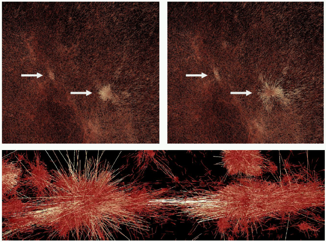
Figure 5: Top two panels: comparison of outputs at $z=10$ using different starting redshifts. The particles are colored with respect to their velocities. The simulation box is 8$\,h^{-1}$Mpc on a side. The simulation shown in the left panel was started at $z_{\rm in}=250$, while for the other, $z_{\rm in}=50$. In the simulation started at $z_{\rm in}=50$, structures formed by $z=10$ are not as concentrated as in simulations with a high-$z$ start, leading to the possible lowering of halo masses. The lower panel shows differences along a filament. In this case a line was drawn between each particle position in the two different data sets. The longer the line, the larger the difference due to the two different initial redshifts. For more details see Haroz et al. (2008); Haroz & Heitmann (2008); Lukić et al. (2007).

We average $P(\bf{k})$ in bins linearly spaced in $k$ of width $\Delta k\simeq 0.001\,{\rm Mpc}^{-1}$, and report this average for each bin containing at least one grid point. We assign to each bin the $k$ associated with the unweighted average of the $k$’s for each grid point in the bin. Note that this procedure introduces a bias in principle, since for nonlinear functions $\langle f(x)\rangle\neq f(\langle x\rangle)$, but our bins are small enough to render this bias negligible.

In a recent paper, Colombi et al. (2008) suggest an alternative approach to accurately estimate power spectra from $N$-body simulations. Their method is based on a Taylor expansion of trigonometric functions as a replacement for large FFTs. The idea is to estimate the power spectrum out to small scales with minimal memory overhead, a major obstacle for the brute force FFT approach. We have checked their method up to fifth order against our results from the $2048^{3}$ FFT and found excellent agreement. Our FFT is clearly large enough to avoid any aliasing at $k\sim 1\,h\,{\rm Mpc}^{-1}$.

5 Initial conditions

The initial conditions in $N$-body codes are often a source of systematic error in ways that can sometimes be hard to detect. It is, therefore, essential to ensure that the implementation of the initial conditions is not a limiting factor in attaining the required accuracy of the power spectrum over the redshift range of interest. An important aspect here is the choice of starting redshift. There are two reasons for this: (i) The Lagrangian perturbation theory used to generate the initial particle distribution (usually the leading order Zel’dovich approximation) is more accurate at higher redshifts, and (ii) for a given (nonlinear) $k$ scale of interest, enough time must have elapsed for the correct nonlinear power spectrum to be established at that scale, at the redshift of interest.

Due to a combination of the two effects mentioned above, delayed starts typically lead to a suppression of structure formation (including the halo mass function) as shown in Figure 5. We now describe our basic methodology for generating initial conditions and choosing the starting redshift.

5.1 Initial Condition Generation

As is standard, we generate our initial conditions by displacing particles from a regular Cartesian grid (“quiet start”) using the Zel’dovich approximation Zel’dovich (1970). In this approximation, the particle displacement and velocity are given by

$${\bf x}(\bf{q}) = {\bf{q}}-D_{1}{{\bf\nabla}}_{q}\phi^{(1)},$$ (5)

$${\bf v}=\frac{d{\bf x}}{dt} = -D_{1}f_{1}H{{\bf\nabla}}_{q}\phi^{(1)}.$$ (6)

Here $\bf{q}$ is the initial (on-grid) position of the particle, $\bf{x}$ is the final position, $D_{1}$ is the linear growth factor defined below in Eqn. (8) and $\phi^{(1)}$ is the potential field. $H$ is the Hubble constant, $f_{i}$ is the logarithmic derivative of the growth function $f_{i}=(d\ln D_{i})/(d\ln a)$, and the time-independent potential $\phi^{(1)}$ obeys the Poisson equation ${\bf\nabla}^{2}_{q}\phi^{(1)}({\bf{q}})=\delta({\bf{q}})$.

A recent suggestion is to determine the initial displacement of the particles and their velocities via second order Lagrangian perturbation theory (2LPT) instead of using the (leading order) Zel’dovich approximation (Scoccimarro, 1998; Crocce et al., 2006). In principle, this could allow a later start of the simulation (lower $z_{\rm in}$) without losing accuracy in the final result. However, it does not address the problem of keeping a sufficient number of expansion factors between the initial and final redshifts. Additionally, error control of the perturbation theory and its convergence properties need to be carefully checked. We have therefore decided on a more conservative approach: instead of using higher order schemes to generate initial conditions, we choose a high enough starting redshift that higher order effects are negligible (see Appendix A). Since most of the code’s runtime is at low redshift, the additional overhead for starting the simulation early is minimal.

The potential field is generated from a realization of a Gaussian random density field $\delta(\bf{k})$ (with random phases). The initial power spectrum is

$$P(k)=Bk^{n}T^{2}(k),$$ (7)

where $B$ determines the normalization and $T(k)$ is the matter transfer function. We compute $T(k)$ using the numerical code CAMB. The results from CAMB were compared against those generated by an independent code described in White & Scott (1996), Hu & White (1997) and Hu et al. (1998). The results from this code are known to agree well with CMBfast Seljak et al. (2003). The final level of agreement was at the $\sim 10^{-3}$ level for the $k$ modes of interest, comfortably below our 1% goal.

The displacement field is easily generated in Fourier space: The Fourier transform of the displacement field is proportional to $({\bf k}/k^{2})\delta({\bf k})$ in the continuum, and we compute the displacements using FFTs. The FFT grid is chosen to have twice as many points, in each dimension, as there are particles.

The scale-independent linear growth factor, $D_{1}(z)$, satisfies (e.g. Peacock, 1999)

$$\left(\frac{D_{1}}{a}\right)^{\prime\prime}+\left(4+\frac{1}{2}\frac{\rho_{c}^{\prime}}{\rho_{c}}\right)\left(\frac{D_{1}}{a}\right)^{\prime}-\left(\frac{3}{2}\frac{\rho_{m}}{\rho_{c}}-\frac{1}{2}\frac{\rho_{c}^{\prime}}{\rho_{c}}-3\right)\left(\frac{D_{1}}{a}\right)=0.$$ (8)

Here $\rho_{c}\propto H^{2}$ is the critical density, $\rho_{m}$ is the matter density and primes denote differentiation with respect to $\ln a$. Our convention has $D_{1}(z=0)\equiv 1$ and $D_{1}(z)\propto(1+z)^{-1}$ when $\rho_{m}\simeq\rho_{c}$. This procedure neglects the differential evolution of the baryons and dark matter, but since we are simulating only collisionless systems here this is the most appropriate choice. Future simulations including baryons will have to deal with this question in more detail.

5.2 The Initial Redshift

The choice of the starting redshift depends on three factors: the simulation box size, the particle loading, and the first redshift at which results are desired. The smaller the box and the higher the first redshift of interest, the higher the initial redshift must be. It is not easy to provide a universal “recipe” for determining the optimal starting redshift. For each simulation set-up, convergence tests must be performed for the quantities of interest. Nevertheless, there are several guiding principles to determine the starting redshift for a given problem. These are:

• Ensure that any unphysical transients from the initial conditions are negligible at the redshift of interest.

• Ensure a sufficient number of expansion factors to allow structures to form correctly at the scales of interest.

• Ensure that the initial particle move on average is much smaller than the initial inter-particle spacing.

• Ensure that $\Delta^{2}(k)\ll 1$ at the wavenumber of interest.

A more detailed description – from a mass function-centric point of view – can be found in Lukić et al. (2007). The aim here is to measure the power spectrum from a (936 $h^{-1}$Mpc)³ box between $z=1$ and $z=0$ at $k=1\,h\,{\rm Mpc}^{-1}$ at 1% level accuracy. In order to fulfill the first and second criteria given above, we generate the initial conditions at $z_{\rm in}$ such that $D(z_{\rm in})/D(z=1)=0.01$. With $D_{1}(z)\simeq a(z)=1/(1+z)$ this leads to a starting redshift of approximately $z_{\rm in}=200$ and one hundred expansion factors between the starting redshift and $z=1$. Note that this criterion is completely independent of the box size and particle loading, though it is cosmology dependent via the growth rate.

For the ($936\,h^{-1}$Mpc)³ boxes we simulate, this starting redshift leads to rms displacements between $3-5\%$ of the mean inter-particle spacing, satisfying the condition that the rms displacement should be much less than the mean inter-particle spacing. This measurement clearly depends on the box size. A smaller box would have led to much bigger displacements with respect to the mean inter-particle spacing. At $z_{\rm in}=200$ the dimensionless power at the fundamental mode is $\mathcal{O}(10^{-8})$ and at the Nyquist frequency is $\mathcal{O}(10^{-4})$ which clearly satisfies the last point of the list above. We show a series of convergence tests including a higher order Lagrangian scheme in Appendix A.

6 Resolution Tests

In order to ensure that our results are properly converged for $k\leq 1\,h\,{\rm Mpc}^{-1}$ between $z=1$ and $z=0$ we need to understand the impact of box size, particle loading, force softening, and particle sampling on the numerically determined power spectra.

6.1 Box Size

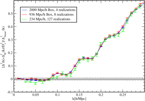
Figure 6: Comparison of power spectra from three different box sizes, $2000\,h^{-1}$Mpc (blue) and $936\,h^{-1}$Mpc (red), and $234\,h^{-1}$Mpc (green). We subtract the initial power spectrum scaled to $z=0$ from the final power spectrum, average over all realizations (4 for the big box, 8 for the medium box, and 127 for the small box), and divide the result by the smooth prediction from linear theory. The error bars show the standard deviation. The overall agreement of $\Delta^{2}(k)$ from the two large box sizes is better than 1% on scales below $k\sim 0.1\,h\,{\rm Mpc}^{-1}$ (the 1% limit is shown by the dotted lines). The small box result displays an overall suppression of the power spectrum at low $k$ (see text).

The choice of the box size depends on several factors. In principle, one should choose as large a volume as practicable, to ensure that the largest-scale modes are (accurately) linear at the redshift of interest (in our case between $z=1$ and $z=0$), improve the statistical sampling (especially for BAO), and to obtain accurate tidal forces. If the box volume is too small, the largest modes in the box may still appear linear at the redshift of interest, even though they should have already gone nonlinear. This leads to a delayed onset of the nonlinear turnover and the quasi-linear regime is treated incorrectly.

Practical considerations, however, add two restrictions to the box size arising from (i) the necessarily finite number of particles, and for the PM simulations, (ii) limitations on the force resolution. The storage requirements and run time for the N-body codes scale (close to) linearly with particle number, so running many smaller boxes “costs” as much as running one very large box with more particles. However the ability to move jobs through the queue efficiently and post-process the data all argue in favor of more smaller jobs than one very large job.

The CDM power spectrum peaks roughly at $k\sim 0.01\,h\,{\rm Mpc}^{-1}$, determined by the horizon scale at the epoch of matter-radiation equality. As the power falls relatively steeply below this value of $k$, a box size of $1\,(h^{-1}$Gpc)³, corresponding to a fundamental mode of $k\sim 0.006\,h\,{\rm Mpc}^{-1}$, is a reasonable candidate for comparing with linear theory on the largest scales probed in the box. [These considerations are of course redshift and $\sigma_{8}$-dependent: at $z=0$, small nonlinear mode-coupling effects can be seen below $k\sim 0.1\,h\,{\rm Mpc}^{-1}$ (cf. Figure 6). At higher redshifts, these effects move to higher $k$.] Of course, bigger boxes are even better (especially for improved statistics, although this is unrelated to linear theory considerations), and a convergence test in box size is described below.

The particle loading is particularly significant as it sets the maximum wavenumber below which the power spectrum can be accurately determined. As discussed in Section 6.2, the accuracy of the power spectrum degrades strongly beyond the Nyquist wavenumber, which depends on both the box size and particle number [see Eqn. (9)]. Therefore, a compromise has to be found between box size and particle loading. After having decided the size of the smallest scale of interest and the maximum number of particles that can be run, the box size is basically fixed. In our case, the optimal solution (considering computational resources) appears to be a box size of roughly 1 $h^{-1}$Gpc on a side and a particle loading of one billion particles – covering a wavenumber range $0.0067\,h\,{\rm Mpc}^{-1}<k<3.4\,h\,{\rm Mpc}^{-1}$ with the upper limit given by the Nyquist wavenumber.

The force resolution for PM codes is a direct function of the box size, once the size of the density (or PM) grid is fixed. While other codes do not have this restriction in principle, PM codes are very fast, and have predictable error properties. In order to obtain sufficient statistics and accuracy for determining $P(k)$, results from many large volume runs at modest resolution can be “glued” to those from fewer high resolution runs, providing an optimal way to sample the quasilinear and nonlinear regimes. PM simulations are very well suited to handling the quasilinear regime; for a Gpc³ box, a 2048³ grid provides enough resolution to match the high-resolution runs out to $k\sim 0.5\,h\,{\rm Mpc}^{-1}$.

In order to ensure that a Gpc³ box is sufficient to obtain accurate results on very large scales, we compare the results from 8 realizations in a (936 $h^{-1}$Mpc)³ box, 4 realizations in a (2000 $h^{-1}$Mpc)³ box, and 127 realizations in a (234 $h^{-1}$Mpc)³ box. The large volume runs were run with 1024³ particles on a 2048³ grid each, the smaller volumes were run with 512³ particles on a 1024³ grid. We subtract the power spectrum from the initial redshift scaled by the growth factor to $z=0$ from the final power spectrum, average over all realizations and divide by the linear theory answer. The results are shown in Figure 6. The agreement between the two sets of large volume simulations is much better than one percent. The agreement with linear theory on scales below $k\sim 0.1\,h\,{\rm Mpc}^{-1}$ is roughly at the percent level and much better than this for $k\sim 0.01\,h\,{\rm Mpc}^{-1}$. We note that for the cosmology used in our study, we do not observe a suppression of the power spectrum with respect to linear theory by $\sim 5\%$ on scales of $0.05\,h\,{\rm Mpc}^{-1}<k<0.075\,h\,{\rm Mpc}^{-1}$ as was reported in, e.g., Smith et al. (2007). The results for the smaller boxes is a few percent below linear theory at large scales and the onset of the nonlinear regime is captured inaccurately. Thus, small box simulations suffer from two defects: first, a large number of simulations is required to overcome finite sampling scatter at low $k$, and, second, all simulations are biased low due to the unphysical suppression of the power spectrum amplitude.

In a recent paper, Takahashi et al. (2008) discuss finite volume effects in detail and propose a way to use perturbation theory to eliminate these effects. They have two concerns: (i) A small simulation volume will lead to enhanced statistical scatter on large scales, if only a few realizations are considered. (ii) If the simulation volume is too small and the linear regime is not captured accurately, the result for the power spectrum will be biased low. We overcome the first difficulty by running many realizations of our cosmological model. In combination with our large simulation volume, we are able to keep the statistical noise below the percent level. The second concern is clearly valid if the simulation box is too small. With the Gpc³ and larger volumes we consider, no size-related bias is observed. The two different box sizes we investigate are in good agreement as can be seen in Figure 6. One concern with respect to the Takahashi et al. (2008) results is that they start their simulations rather late ($z_{\rm in}=30$) and investigate the results starting at $z=3$. As demonstrated in Figure 17 such a late start suppresses the power spectrum at quasilinear and nonlinear scales.

6.2 Mass Resolution

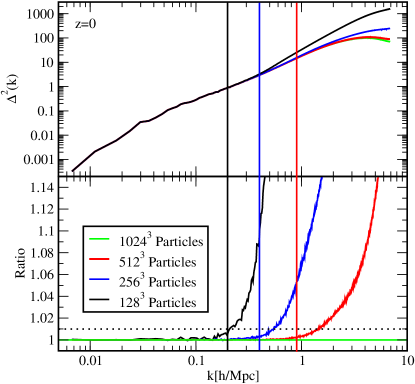
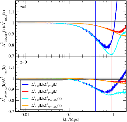
Figure 7: Importance of particle sampling for calculating the power spectrum. The underlying simulation is the GADGET-2 run with 1024³ particles. All power spectra are measured on a 2048³ grid. Upper panel: green – power spectrum from 1024³ particles at $z=0$, red – from the 512³ downsampled distribution, blue – from the 256³ downsampled distribution, black – from the 128³ downsampled distribution. Vertical lines denote $k_{\rm Ny}/2$ for the three cases: 128³ (black), 256³ (blue), 512³ (red). Lower plot: ratios of the downsampled power spectra with respect to the 1024³ particle power spectrum. The dotted line represents the 1$\%$ deviation limit.

Figure 8: Mass resolution test. The 1024³ particle ICs have been downsampled to 512³ and 256³ particles and run to $z=0$. The plot shows the ratio of the obtained power spectra at $z=1$ (upper panel) and $z=0$ (lower panel) with respect to the full 1024³ power spectrum at $z=0$ (blue, red) and the power spectra which are obtained by downsampling the particles at $z=0$ (turquoise, orange; see also Figure 8). The vertical lines mark $k=k_{\rm Ny}/2$ for the two cases.

We investigate the influence of the particle loading on the accuracy of the power spectrum by first asking the following question: How many particles are required to sufficiently sample the density field when calculating the power spectrum? To answer this question we start from one of the GADGET-2 simulations run with a ($936\,h^{-1}$Mpc)³ box and with 1024³ particles. We determine the power spectrum from this run at $z=0$. Next, we downsample the $1024^{3}$ particles to $512^{3}$, $256^{3}$, and $128^{3}$ particles by taking the particles which belong to every second (fourth, eight) grid point in each dimension. Since the particles are downsampled from a fully evolved simulation, evolution and sampling issues are separated.

In the upper panel of Figure 8 the resulting power spectra are shown. The lower panel shows the ratio of the power spectra from the downsampled distributions with respect to the 1024³ particle distribution. In addition, we have marked the Nyquist wavenumber divided by two for each power spectrum. The Nyquist wavenumber is set by the inter-particle separation on the initial grid:

$$k_{\rm Ny}=\frac{\pi}{\Delta_{p}}=\frac{\pi N_{p}}{L},$$ (9)

with $\Delta_{p}$ being the inter-particle spacing, $N_{p}$ the cube-root of the number of particles, and $L$, the box size ($936\,h^{-1}$Mpc)³. Values of $k_{\rm Ny}$ for the $1024^{3}$, $512^{3}$, $256^{3}$, and $128^{3}$ particle cases are 3.4, 1.71, 0.86, and $0.43\,h\,{\rm Mpc}^{-1}$, respectively. As shown in Figure 8, all power spectra agree to better than 1% for $k<k_{\rm Ny}/2$. The undersampled particle distributions lead to an overprediction of the power spectrum beyond this point due to the increase in particle shot noise. As mentioned earlier, a simple shot noise subtraction assuming Poisson noise as given in Eqn. (4) does not compensate for this increase. Detailed tests show that the shot noise which leads to the overprediction is scale-dependent and smaller than Poisson shot noise on the scales of interest. (A naive Poisson shot noise subtraction would alter the power spectrum at $k=1\,h\,{\rm Mpc}^{-1}$ by 0.2% at $z=0$ and by 1% at $z=1$ for 1024³ particles.) Thus we are led to conclude that, in the absence of shot noise modeling (a difficult and potentially uncontrolled procedure), the one-percent accuracy requirement on the power spectrum can only be satisfied for wavenumbers, $k<k_{\rm Ny}/2$. This quite restrictive limit likely comes from the fact that the power spectrum is sensitive to near-mean-density material which is not well modeled on scales smaller than the mean inter-particle separation.

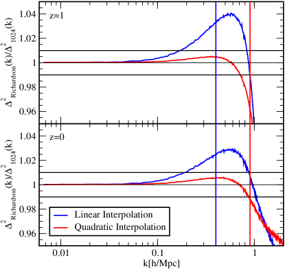
Figure 9: Richardson extrapolation test. Assuming linear [blue curve, Eqn. (B5)] and quadratic convergence [red curve, Eqn. (B7)], the 256³ and 512³ particle results are used to predict the power spectrum for the 1024³ particle run. Both plots show the ratio of the prediction with respect to the true result. The quadratic extrapolation works well in the regime below the half-Nyquist wavenumber, to sub-percent accuracy. At $k=1\,h\,{\rm Mpc}^{-1}$ the quality deteriorates due to the insufficient resolution of the two underlying runs (Cf. Figure 8). The vertical lines are the same as in Figure 8.

The next step is to investigate how the error from an “undersampled” initial particle distribution propagates through the numerical evolution. For this test we first downsample the initial particle distribution in the same way as before, at $z_{\rm in}=211$, from the original $1024^{3}$ particles to $512^{3}$ particles and $256^{3}$ particles. We then run the simulations to $z=0$ with the same settings in GADGET-2 as were used for the full run ($2048^{3}$ PM grid and a softening length of $50\,$kpc). We do not use the $128^{3}$ particle set for this test since the corresponding sampling error is too large. Results are shown in Figure 8 for outputs at $z=1$ and $z=0$. Ratios of the power spectra from the downsampled initial conditions (ICs) are shown with respect to: (i) the power spectrum from the full $1024^{3}$ run, and (ii) the power spectra correspondingly downsampled at $z=1$ and $z=0$ as shown in Figure 8.

There are two points to note here. First, restricting attention to case (i) above, there is a noticeable loss of power below $k_{\rm Ny}$, and second, a steep rise beyond this point. The loss of power is not due to the downsampling in the initial condition – as can be easily checked by comparing the power spectrum from the particles after the IC generation against the desired input power spectrum for the given realization – but is due to a discreteness effect: a reduction in the linear growth factor from its continuum value as $k\rightarrow k_{\rm Ny}$. As the evolution proceeds, this suppression is reduced due to the addition of nonlinear power, as can be seen by comparing the $z=1$ and $z=0$ results in Figure 8, and also by noting the smaller suppression for the case with $512^{3}$ particles for which the larger $k_{\rm Ny}$ means an enhancement in nonlinearity (cf. Figure 8). The steep rise is a manifestation of particle shot noise as can be seen by looking at the results for case (ii). For wavenumbers up to $k_{\rm Ny}/2$ there is no difference between the two ratios [case (i) vs. case (ii)] but beyond that point the results from case (ii) show a marked reduction ($z=1$) to almost a removal ($z=0$) of the enhancement, consistent with the stated hypothesis. We would like to re-emphasize that our convergence tests show that a Poisson shot noise subtraction alters the power spectrum in the wrong way at the scales of interest. It enhances the suppression of the power spectrum near the Nyquist wavenumber and overcorrects the power spectrum at higher wavenumbers.

The problem we now face is that the (IC downsampling) error at $k\sim k_{\rm Ny}/2$ is large: for the $256^{3}$ particle run at $z=1$ it is $\sim 20\%$, and for $512^{3}$ particles it is still $\sim 7\%$. At $z=0$, the error is $\sim 10\%$ for the $256^{3}$ run and $\sim 3\%$ for the $512^{3}$ run. Thus, one may wonder if the fiducial $1024^{3}$ particle run can itself yield results at $k=1\,h\,{\rm Mpc}^{-1}$ accurate to 1%.

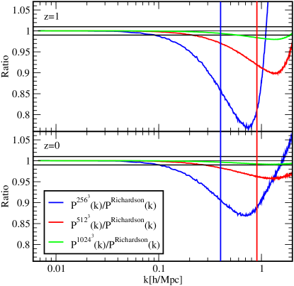
Figure 10: Mass resolution convergence study with respect to the extrapolation results at $z=1$ and $z=0$. The content of this figure is very similar to that of Figure 9, but here we show results with respect to the 2048³ particle prediction from the (quadratic) Richardson extrapolation. This allows us to investigate the convergence properties of the 1024³ particle runs (see text for details). The vertical lines are the same as in Figure 8.

A brute force approach would be to run with 2048³ particles and check convergence with respect to that simulation. To avoid the computational cost of the brute force approach, we take a different tack: We extrapolate from the two low-mass resolution runs to try and predict the results of the high-mass resolution run (see Appendix B). The success of Richardson extrapolation when applied to power spectra from different force resolution runs has been demonstrated by Heitmann et al. (2005). We now carry out a similar procedure, allowing for both linear or quadratic convergence.

Figure 9 shows the results for the extrapolation tests for $z=1$ and $z=0$. Following Eqns. (B5) and (B7), we assume linear and quadratic convergence respectively, and predict the power spectrum for the 1024³ particle run, displaying the ratio of the prediction with respect to the full 1024³ run. The quadratic extrapolation scheme works much better than the linear one – out to $k\simeq 0.8\,h^{-1}$Mpc the prediction is accurate to better than 1%. Obviously, the prediction will not work very well beyond the scale set by the mass resolution of the 256³ simulation. Nevertheless, the test shows that at $k=1\,h\,{\rm Mpc}^{-1}$ (which is close to $k_{\rm Ny}/2$ from the $512^{3}$ particle run and below $k_{\rm Ny}/2$ for the $1024^{3}$ particle run), we should obtain a reasonably accurate prediction for a $2048^{3}$ particle run.

Figure 10 shows that the $1024^{3}$ particle run is within 1% of the prediction for a $2048^{3}$ run to $k\simeq 1\,h\,{\rm Mpc}^{-1}$ at $z=0$ and within 2-3% at $z=1$ (but here the extrapolation scheme itself is being stretched to its limit – the actual result is likely to be better). This enables us to conclude that our mass resolution will allow a 1% accurate calculation at the scale of interest, without any need to extrapolate.

6.2.1 Aliasing Effects

To confirm the results of the tests in this section, we check here for possible aliasing artifacts which might arise since $N_{p}\neq N_{g}$ in the initial conditions ($N_{g}$ is the number of grid points per dimension). We will show briefly in the following that such effects are negligible.

As explained in Section 5.1, the initial conditions in our simulations are set in the following manner: (i) Implement a realization of a Gaussian random field initial condition for the density field in $k$-space, and also for the corresponding scalar potential and gradients of the potential. (ii) Using an inverse FFT, determine the gradient field in real space, and use it to move particles from their initial on-grid positions (where the potential gradient is exactly known) using the Zel’dovich approximation. Aliasing cannot enter in the first inverse FFT, but it can in the second, “particle move” step, since the particle grid is not constrained to be the same as the field grid.

In most simulations, with some exceptions, the typical choice for the initial condition is to take $\Delta_{p}=\Delta_{g}$ or $\Delta_{p}=2\Delta_{g}$ ($\Delta_{g}$ is the grid spacing) since there is not much point in adding field power that cannot be represented by the particle distribution (beyond a spatial frequency set by the particle Nyquist wavenumber $k_{\rm Ny}$). In addition there is a question that doing this could be a problem for simulations by leaking artifical “grid” power into the initial conditions.

In reality, the situation is relatively benign because of the rapid fall-off of the initial $P(k)$ at high $k$. This can be seen in results from earlier papers, e.g., Baugh et al. (1995), Fig. A.3. Modern simulations have much higher mass and force resolution, so it is important to check each time one runs simulations, that there is no problem with aliased or some other artificial power leaking back to lower $k$.

The central issue is the existence of the first particle grid peak in the power spectrum at $k_{p}=2\pi/\Delta_{p}$ which influences the computation of $P(k)$ close to it in a way that is hard to correct or compensate for, given that we are interested in percent level accuracy. For a chosen $k$ scale of interest, $k_{I}<k_{\rm Ny}$, one has to make sure that $k_{p}$ is sufficiently greater than $k_{I}$ at the redshift of interest [the lower the redshift the easier to satisfy this condition, since evolution boosts $P(k_{I})$ significantly compared to $P(k_{p})$].

In the specific mass resolution tests carried out above we investigate the case of a single realization with fixed $\Delta_{g}$ for different choices of $\Delta_{p}$. In order to show that potential aliasing effects do not alter our results we carry out the following additional test. We fix $N_{g}=1024$ and consider two cases with $N_{p}=512$ and $N_{p}=256$ (corresponding to $\Delta_{p}=2\Delta_{g}$ and $\Delta_{p}=4\Delta_{g}$). In addition to these runs we also run three simulations all with $\Delta_{p}=\Delta_{g}$ with $N_{p}=1024$, $N_{p}=512$, and $N_{p}=256$, explicitly setting all the high-$k$ modes to zero for the latter two cases, for the same $k$ space realization as in the first. Thus we have essentially the same phases but no power beyond $k_{\rm Ny}$ in all three cases. The results for $P(k)$ are shown at $z=0$ as a ratio against the $N_{g}=N_{p}=1024$ case in Figure 11. Note that the same suppression of power around $k_{\rm Ny}$ as noted in the previous section is seen here, independent of whether high $k$ power is present in the initial conditions or not. Thus any effect due to aliasing is negligible.

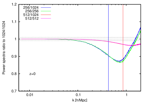
Figure 11: Ratio of power spectra showing insensitivity to the presence of $k>k_{\rm Ny}$ power in the initial conditions. Note the excellent agreement between the 256/256 and 256/1024 runs and the 512/512 and 512/1024 runs. The vertical lines denote $k_{\rm Ny}/2$ for the two cases.

6.3 Force Resolution

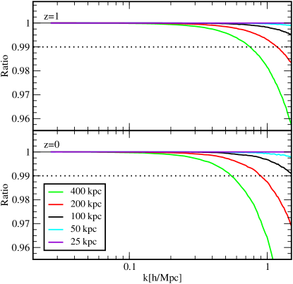
Figure 12: Force resolution convergence study at $z=1$ and $z=0$ with GADGET-2. The 512³ PM grid is the same in all five runs, and the force resolution is varied between 25 kpc and 400 kpc. At $k\sim 1\,h\,{\rm Mpc}^{-1}$, a force resolution of 100 kpc already leads to results converged well below 1% at both redshifts with respect to the 25 kpc resolution run.

As discussed in Section 3 we employ two $N$-body methods in this paper: PM simulations with grid sizes of 1024³ and 2048³ and tree-PM simulations. The force resolution of the PM runs is insufficient to resolve the power spectrum out to $k\sim 1\,h\,{\rm Mpc}^{-1}$ (see, e.g., Figure 14 for the shortfall of power in the PM runs). We therefore discuss only the convergence properties of the tree-PM algorithm out to $k~{}\sim 1\,h\,{\rm Mpc}^{-1}$. Since the GADGET-2 runs with $1024^{3}$ particles are computationally expensive, and the force softening primarily affects small scales, we chose to downscale the simulation box and number of particles for this test to $256^{3}$ particles in a $234\,h^{-1}$Mpc box (a reduction by a factor of 64 from the main runs). Following the practice in the larger runs, the PM force grid is set to twice the number of particles in one dimension, resulting in a $512^{3}$ PM mesh. All the other code settings are the same as for the large runs and we vary only the force softening to test for the effects of finite force resolution. The effective force resolution lengths range from $400\,$kpc to $25\,$kpc ($50\,$kpc is used in the large runs). The results for $z=0$ and $z=1$ are shown in Figure 12. At $k\sim 1\,h\,{\rm Mpc}^{-1}$, the difference between $50\,$kpc and $25\,$kpc is well below 0.1% for both redshifts, and therefore comfortably within our requirements. In fact, meeting the force resolution requirements at $k\sim 1\,h\,{\rm Mpc}^{-1}$ with the tree-PM algorithm is computationally much less demanding than meeting the mass resolution requirements. It may be that for power spectrum simulations a hybrid or adaptive PM code is the most computationally efficient route, though other uses of the simulations may be more sensitive to resolution.

The size of the PM mesh is a separate issue, and significant in its own right. If high accuracy is desired the mesh should not be chosen to be too small, as this increases the PM error and pushes the handover between the tree and the mesh to larger scales. In tests carried out to determine the size of the PM grid, we observed an unphysical suppression of the early-time power spectrum at quasi-linear scales for the smaller meshes.

6.4 Time Stepping

Most $N$-body codes use low-order – typically, second order – symplectic time-stepping schemes. (Full symplecticity is not achieved when adaptive time-stepping is employed.) The choice of the time variable itself can vary, although typically it is some function of the scale factor $a$, e.g., $a$ itself or the natural logarithm of $a$. PM codes most often use constant time stepping in $a$ or $\ln a$. Higher-resolution codes use adaptive, as well as individual particle time-stepping. Hybrid codes that mix grid and particle forces, such as tree-PM, have different criteria for time-stepping the long-range forces as compared to the short-range forces, where individual particle time-steps are often used. Because of these complexities, it is important to check that the time-stepping errors are sub-dominant at the length-scales of interest for computing the mass power spectrum.

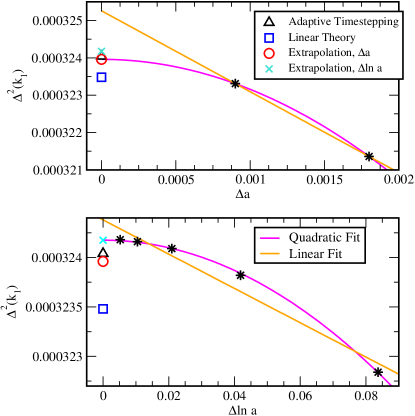
Figure 13: Time stepper convergence for $\Delta^{2}(k)$ using linear (upper plot) and logarithmic (lower plot) time-stepping in $a$ at $z=0$, as a function of number of time steps. The $k$ value chosen is for the largest mode in the box, $k=6.7\times 10^{-3}\,h\,{\rm Mpc}^{-1}$ (black stars). The black triangle shows the result from a GADGET-2 run with adaptive time stepping in $\ln a$, the blue box is the power spectrum from the initial condition scaled by the linear growth factor to $z=0$, the red circle the $\Delta^{2}(k)$ value for time-stepping linear in $a$ extrapolated to zero assuming quadratic convergence, and the turquoise cross the same quantity for $\ln a$. All (extrapolated) values from the simulations agree with linear theory to 0.2% or better, the simulations themselves agreeing to better than 0.04% taking the GADGET-2 run as the reference. The pink line shows a quadratic fit to the data points.

The GADGET-2 runs in this paper use $\ln a$ as the time variable. The PM calculations within GADGET-2 use a global time step; we found 256 time steps sufficient for this part. The tree algorithm for the short-range forces uses an adaptive time stepping scheme and our runs use a total of about 3000 time steps. The criterion for the adaptive time stepping is coupled to the softening length $\epsilon$ via : $\Delta t=\sqrt{2\eta\epsilon/|a|}$ where $\eta$ allows adjustments in the time stepping; we use $\eta=1\%$ (note that here $a$ is the acceleration). Detailed tests of the convergence of the time stepping employed by GADGET-2 can be found in Section 4 of Springel (2005).

We perform an additional test to verify the expected quadratic convergence, considering the largest mode in the box (in this case $k=6.7\times 10^{-3}\,h\,{\rm Mpc}^{-1}$). We compare the numerical results for $P(k)$ with that expected from linear theory, which should be reasonably accurate at these very large scales. By using the largest mode, one is insulated from errors due to the particle loading and small-scale force resolution.

We investigate both time variable choices, $\ln a$ and $a$. The results are shown in Figure 13. All the test runs are in pure PM mode on a $1024^{3}$ grid, with the tree switched off in GADGET-2 (there is no need for high force resolution in this test) and using global time-stepping. For steps linear in $a$ we show results for roughly 600 and 1,200 time steps, for the time stepper in $\ln a$ we show results for $\Delta\ln a\approx$ 0.005, 0.01, 0.02, 0.04, and 0.08. In addition, we fit two curves through the results assuming linear and quadratic convergence. As expected from a second order integrator, the quadratic fit is in very good agreement with the data points. Quadratic extrapolation of the results for the two time stepping schemes from finite $k$ to zero is in very good agreement with linear theory, to better than 0.2% – about the deviation expected given the dimensionless power at the fundamental mode of the box. If we take the adaptive time step run as the reference (rather than linear theory), the agreement is better than 0.04%. Adaptive time-stepping is expected to yield results very close to $\ln a$ stepping on large scales, since for the long-range force even the adaptive time-stepper run is constant in $\ln a$ with $\Delta\ln a=0.02$. The excellent agreement with time-stepping in $a$ confirms the robustness of the different schemes. Since our interest is in generating the power spectrum at percent accuracy at minimal computing cost, we conclude that the $\ln a$ time-stepping scheme with approximately 250 time steps is a good compromise for the PM runs to obtain an accurate power spectrum at quasi-linear scales (two orders of magnitude removed from scale set by the force resolution).

7 Matching low and high resolution power spectra and comparison with HaloFit

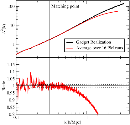
Figure 14: Matching of an ensemble of low resolution runs with one realization of a high-resolution GADGET-2 run. The upper panel shows the average from 16 realizations from the low resolution PM runs (red) and the power spectrum from the GADGET-2 run (black). The lower panel shows the ratio of the low resolution ensemble with respect to the GADGET-2 run. Out to $k\sim 0.5\,h\,{\rm Mpc}^{-1}$ the difference is less than one percent (disregarding the noise from the single realization). We match the two power spectra at $k\sim 0.3\,h\,{\rm Mpc}^{-1}$, at which point the noise in the single realization is small enough, yet the resolution of the PM runs is sufficient to accurately resolve the power spectrum.

Last, we compare our results with the standard fitting formula, HaloFit (Smith et al., 2003), currently used for analysis of e.g. weak lensing data (Jarvis et al., 2006; Massey et al., 2007; Benjamin et al., 2007; Fu et al., 2008) or for forecasts on the improvement of cosmological constraints from future surveys (Tang et al., 2008). HaloFit provides the nonlinear power spectrum over a range of cosmologies in a semi-analytic form. It is based on a combination of the halo model approach (for a review of the halo model, see e.g., Cooray & Sheth 2002) and an analytic description of the evolution of clustering proposed by Hamilton et al. (1991). In addition, the fit is tuned to simulations by introducing two new parameters: an effective spectral index on nonlinear scales, $n_{\rm eff}$, and a spectral curvature $C$. The combination of analytic arguments and tuning to results from $N$-body simulations has led to the most accurate fit for the nonlinear power spectrum to date (as we will show below, the fit is accurate to $\sim 5-10$%). As mentioned above, we use here the CAMB implementation of HaloFit.

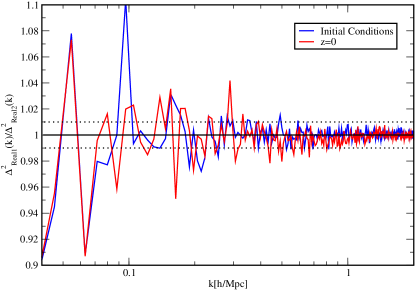
Figure 15: Ratio of power spectra from two independent realizations at initial and final redshifts. Both simulations are carried out with GADGET-2 at the standard setting. Results as shown have been smoothed by averaging over every five $k$-values. Beyond our matching point for low and high resolution simulations, $k=0.3$ $h$Mpc^-1, the results agree at the percent level, confirming that one realization of an $\sim h^{-1}$Gpc high-resolution run is sufficient.

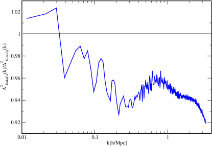
Figure 16: Comparison of the simulation power spectrum to HaloFit. Shown is the ratio of HaloFit with respect to the simulation result. The simulation result has been obtained by combining the PM runs and the GADGET-2 run at $k=0.3\,h\,{\rm Mpc}^{-1}$ and it has been smoothed by averaging over every five $k$-values to reduce the noise for the comparison. The HaloFit result is approximately 5% lower than the result from simulations.

In order to compare simulation results to a smooth fit, we first combine 16 realizations from the PM runs in the low $k$ region with one high-resolution run, as shown in Figure 14. At around $k=0.6\,h\,{\rm Mpc}^{-1}$ the lower resolution of the PM runs begins to become apparent and the result falls below that from GADGET-2. Conservatively, we match the two power spectra at $k=0.3\,h\,{\rm Mpc}^{-1}$. At this point, the variance from the single realization of the GADGET-2 run is small enough that the matching leads to a smooth power spectrum. (A more sophisticated matching procedure is described in Lawrence et al. 2009, Paper III.) One concern might be that a single realization is insufficient to capture the behavior on small scales accurately: Because of mode coupling it is not obvious that fluctuations on large scales do not also cause substantial effects on small scales. In Figure 15 we show that, due to the large box size, this is not a concern at least at the percent level of accuracy. The figure shows the ratio of two different realizations at the initial and final redshift. Both simulations are run with GADGET-2 at our standard settings. The variations at high $k$ (beyond the matching point $k=0.3\,h\,{\rm Mpc}^{-1}$ ) are at the percent level and appear to be free of systematic trends.

The ratio of the matched power spectrum to the prediction from HaloFit is shown in Figure 16. In this case, the HaloFit prediction falls roughly 5% below the simulation. The procedure for combining the simulation results can be seen to work very well, as there is no discontinuity at $k=0.3~{}h$Mpc^-1 from the matching. Our result is in good agreement with, e.g., Smith et al. (2008) as well as Ma (2007), who find a 5% supression for HaloFit at $k\sim 0.1~{}h$Mpc^-1. At larger $k$, however, the results in Ma (2007) may not be very accurate, due to limitations in force resolution in that work.

8 Conclusion and Outlook

The advent of precision cosmological observations poses a major challenge to computational cosmology. With observational results accurate to the percent level a significant uncertainty in extracting cosmological information from the data is due to inaccuracies in theoretical templates. At the required level of accuracy large scale simulations are unavoidable, since the nonlinear nature of the problem makes it impossible to derive analytic or semi-analytic expressions for statistics such as the matter power spectrum, at an accuracy better than $\sim 10\%$. While simulations in principle should yield results at sub-percent accuracy, in practice this is a non-trivial task due to uncertainties in the numerical implementation and modeling of relevant physical processes.

Motivated by this realization, we decided to carry out an end-to-end calculation of one of the simplest non-trivial problems we could imagine: a percent level computation of the nonlinear mass power spectrum to $k\sim 1\,h\,{\rm Mpc}^{-1}$ over the range $0<z<1$. This was a problem which appeared useful and timely as well as tractable (if not straightforward) while still providing a meaningful learning environment – by actually going through all of the steps we would map out the necessary infrastructure which would be required, find the most difficult pieces of the problem and present a proof-of-principle demonstration that meaningful, precision theoretical predictions could be used in support of future cosmological measurements.

We have broken the problem into three steps, to be presented in three publications. In this, first, paper we showed that it is possible to obtain a calibration of the nonlinear matter power spectrum at sub-percent/percent accuracy out to $k\sim 1\,h\,{\rm Mpc}^{-1}$ between $z=1$ and $z=0$. This wavelength regime is important for ongoing and near-future weak-lensing surveys. The restriction to these (large) length scales has two major advantages: baryonic effects are subdominant on these scales (e.g. White, 2004; Zhan & Knox, 2004; Jing et al., 2006; Rudd et al., 2008; Guillet, Teyssier & Colombi, 2009) and the numerical requirements in this regime remain rather modest. Each simulation can be carried out in a matter of days on parallel computers with several hundred processors and the data volume is manageable with arrays of inexpensive disk. Pushing beyond $k\sim 1\,h\,{\rm Mpc}^{-1}$ will require advances in our understanding of the implementation of baryonic physics, or self-calibration techniques, as well as advances in algorithms and computational power.

We derived a set of numerical requirements to obtain an accurate power spectrum by performing a large suite of convergence and comparison tests. The goal was a set of code settings which balance the need for precision and the limitation of computational resources. As shown here, the simulation volume and, especially, the particle loading are two major concerns in obtaining an accurate matter power spectrum. The simulation volume has to be in the $\sim$Gpc³ range, leading to a minimum requirement of $\sim 1$ billion particles. Further increase in volume would be helpful, but would require a concomitant increase in the number of particles, greatly adding to the computational burden. The 1 Gpc³/1 billion particle simulation is a good compromise between sufficient accuracy and computational cost.

Besides a large simulation volume and good particle sampling, initialization of the simulation also plays an important role. To guarantee converged results, the simulation must be started at a high enough redshift. We found that a starting redshift of $z_{\rm in}\simeq 200$ is sufficient to get accurate results between $z=1$ and $z=0$.

The results for the power spectrum are rather stable to changes in the number of time steps. This is clearly related to the fact that our resolution demands are relatively modest. For the PM runs, a few hundred time steps are sufficient, while for the tree-PM runs the overall number of time steps is a factor of ten larger. We emphasize that the simulation settings discussed here will lead to the required accuracy only up to $k\sim 1\,h\,{\rm Mpc}^{-1}$. While these settings can be used as a guideline for other simulation aims, they do not replace convergence tests that must be performed for each new problem, if one desires high precision results.

While weak lensing was a primary motivation for this study, our efforts are of wider interest as an exercise in precision “theoretical” cosmology. We demonstrated that it is possible to achieve 1% accuracy in the mass power spectrum in gravity only simulations on relatively large scales for a limited range of cosmological models. Had this not been the case the field would have needed to rethink its demands on theory. The non-trivial computational and human cost of even this “first step” argues for increased efforts in these directions in order to satisfy the increasingly stringent demands of future observations.

Having established the ability to generate power spectra with sufficient accuracy from $N$-body simulations, the next major question that arises is how to use these costly simulations for parameter estimation, e.g., via Markov Chain Monte Carlo. To address this problem, we have recently introduced the cosmic calibration framework (Heitmann et al., 2006; Habib et al., 2007; Schneider et al., 2008) which is based on an interpolation scheme for the power spectrum (or any other statistic of interest) derived from a relatively small number of training runs.

The next step in generating precise predictions for the matter power spectrum is to determine the minimum number of cosmological models needed to build an accurate emulator and then to construct the emulator from a set of high-precision simulations. In the second paper of this series we establish that 30-40 cosmological models are sufficient to explore the parameter space for $w$CDM cosmologies (constant $w$) given the current constraints on parameter values. The third and final paper will present results from the simulation suite designed and discussed in the second paper, and will include a power spectrum emulator that will be publicly released.

Appendix A Convergence Tests for Initial Conditions

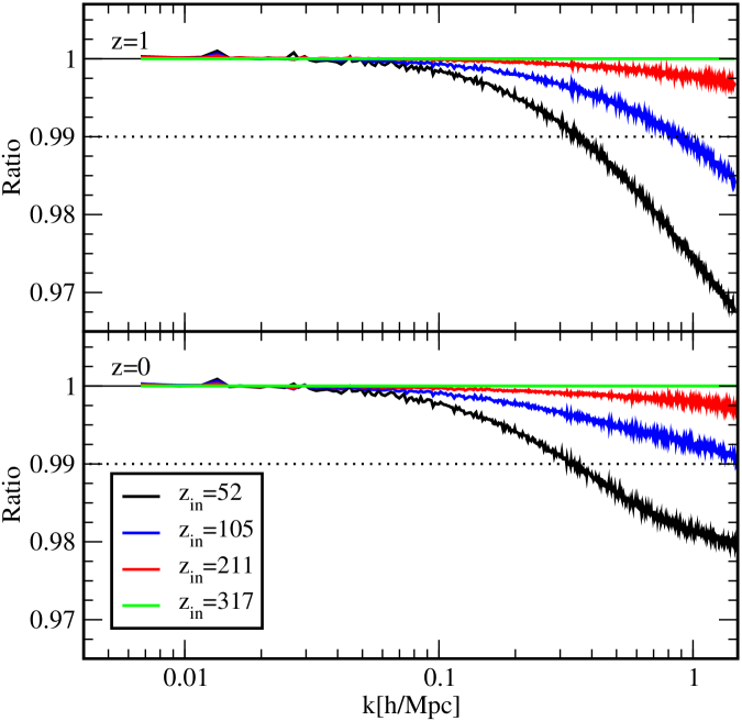
Figure 17: Comparison of ratios of the dimensionless power spectra at $z=1$ (upper panel) and $z=0$ (lower panel) when evolved using a PM code from initial conditions generated using the Zel’dovich approximation at the starting redshifts indicated. The rms displacement for the starts is 0.335, 0.168, 0.084, and 0.055 times the mean inter-particle spacing (for $z_{\rm in}=52$, 105, 211 and 317). The dotted lines mark the 1% limit. If the code is started at $z_{\rm in}=52$, we see a suppression of the power spectrum by $\sim 3\%$ at $z=1$ and $\sim 2\%$ at $z=0$.

The initial conditions for $N$-body simulations are usually generated by displacing particles from a regular grid using the Zel’dovich approximation. This amounts to a first order expansion in Lagrangian perturbation theory. In order to verify that our criteria for the initial redshift, explained in Section 5, are sufficient to guarantee one percent accuracy between $z=1$ and $z=0$ we carry out a convergence study.

The first step is indicated in Figure 17, which shows that the power spectrum between $z=1$ and 0 converges as we increase $z_{\rm in}$ and is well converged by $z=0$ given $z_{\rm in}$ satisfying our criteria. Our results are in very good agreement with similar tests carried out by, e.g., Ma (2007). We carried out numerous other tests with very similar results including tests for different cosmologies. By starting when $D(z_{\rm in})/D(z=1)=0.01$ our results are converged to better than $1\%$ for all $0\leq z\leq 1$.

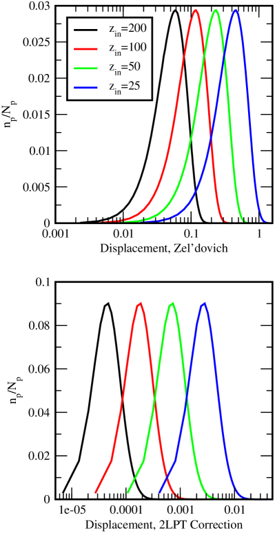
Figure 18: Upper panel: distribution of the initial displacements of all particles at different starting redshifts ($z_{\rm in}=200,~{}100,~{}50,~{}25)$. The displacement is measured with respect to the mean inter-particle spacing. For $z_{\rm in}=200$, the rms displacement is approximately 0.05, while for $z_{\rm in}=25$ it increases by a factor of ten. Lower plot: 2LPT correction. The distributions show the additional contribution in the initial move to the Zel’dovich approximation. For $z_{\rm in}=200$ this additional move is on average $4\cdot 10^{-5}$ and for $z_{\rm in}=25$ it is 0.004 of the mean inter-particle spacing. In both cases this is a small fraction with respect to the Zel’dovich move. In both plots, the $y$-axis is scaled with respect to all particles.

Figure 19: Power spectra ratios for four different initial redshifts. The initial power spectrum obtained from Zel’dovich initial conditions is divided by the power spectrum from the 2LPT initial conditions. Overall, the Zel’dovich initial conditions have slightly less power on the smallest scales. Results are shown out to $k_{\rm Ny}/2=\pi N_{p}/2L=1.57\,h\,{\rm Mpc}^{-1}$. Remarkably, even if the initial conditions are generated as late as $z_{\rm in}=25$, the difference in the power spectra is below 1% at the smallest scales. For $z_{\rm in}=200$, the difference on all scales is far below one percent. Nishimichi et al. (2008) found a similar result: sub-percent agreement between power spectra from the Zel’dovich approximation and 2LPT initial conditions at $z=127$.

The second step is to show that the results as $z_{\rm in}\to\infty$ are converging to the desired answer. One way to check this is to compare the ZA scheme to a higher order Lagrangian approximation, e.g. $2^{\rm nd}$ order Lagrangian perturbation theory: 2LPT. (The use of a higher order Lagrangian approximation scheme to set up initial conditions has been suggested recently, e.g., Crocce et al. 2006.) For small initial perturbations 2LPT should be more accurate than ZA, and generates transients which decay much faster with the expansion of the Universe ($a^{-2}$ rather than $a^{-1}$). In the 2LPT formalism, the particle displacement is obtained in second order Lagrangian perturbation theory, an additional contribution being added to that from the Zel’dovich approximation as given in Eqn. (5):

$$\bf x(\bf q) = {\bf q}-D_{1}{\bf\nabla}_{q}\phi^{(1)}+D_{2}{\bf\nabla}_{q}\phi^{(2)},$$ (A1)

$$\bf v = \frac{d{\bf x}}{dt}=-D_{1}f_{1}H{\bf\nabla}_{q}\phi^{(1)}+D_{2}f_{2}H{\bf\nabla}_{q}\phi^{(2)},$$ (A2)

where $\phi^{(2)}$ is obtained from solving

$${\bf\nabla}^{2}_{q}\phi^{(2)}({\bf q})=\sum_{i>j}\left\{\phi_{,ij}^{(1)}({\bf q})\phi^{(1)}_{,ij}({\bf q})-[\phi^{(1)}_{,ij}({\bf q})]^{2}\right\}$$ (A3)

and $D_{2}$ is the second order growth function. In the following, we investigate the contributions from the second terms in the positions and velocities of the particles at different redshifts.

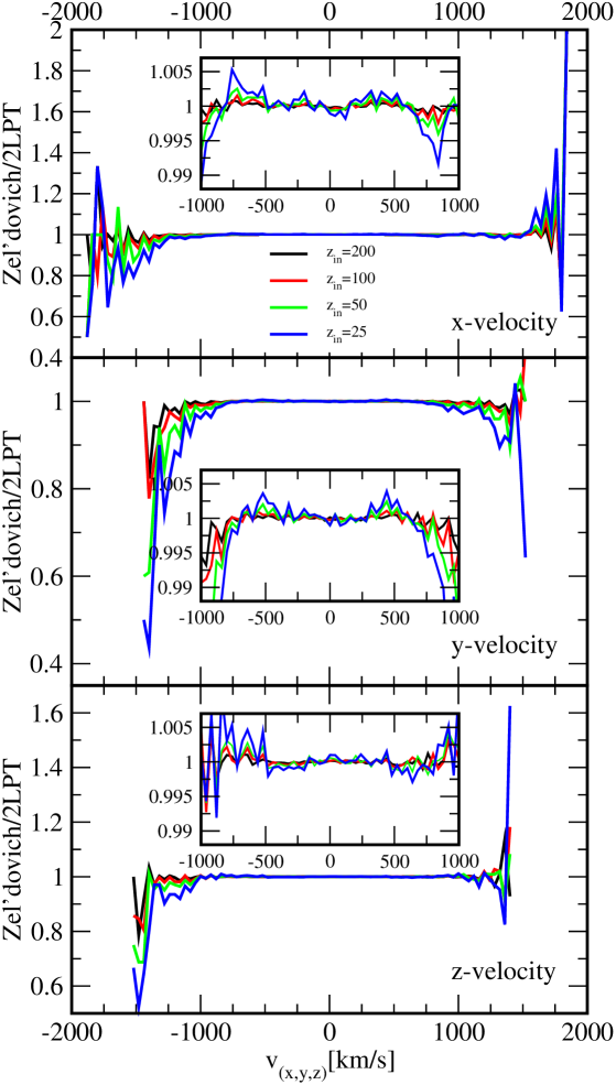
Figure 20: Ratio of histograms of the three velocity components from the Zel’dovich approximation and the 2LPT approach. The insets show the regimes between -1000 km/s and 1000 km/s where the large majority of the particles reside. Here the difference is sub percent. The different colors represent different starting redshifts, the difference becoming smaller for higher redshift starts.

Crocce et al. (2006) have made a serial 2LPT code publicly available. Their code uses approximations for the growth functions in first and second order. (In contrast, the ZA initialization routine used for this paper solves the differential equation for the linear growth function directly, without making approximations.) For a $\Lambda$CDM cosmology these approximations are given by:

$$D_{1} \approx \frac{5}{2}a\Omega_{m}\left[\Omega_{m}^{4/7}-\Omega_{\Lambda}+\left(1+\frac{\Omega_{m}}{2}\right)\left(1+\frac{\Omega_{\Lambda}}{70}\right)\right]^{-1},$$ (A4)

$$D_{2}(\tau) \approx \frac{3}{7}D_{1}^{2}(\tau)\Omega_{m}^{-1/143}\approx-\frac{3}{7}D^{2}_{1}(\tau),$$ (A5)

with $\tau$ being conformal time. The approximation for $D_{1}$ can be found in Carroll et al. (1992). For $f_{1}$ and $f_{2}$ the following approximations are made:

$$f_{1}\approx\Omega_{m}^{5/9},~{}~{}~{}f_{2}\approx 2\Omega_{m}^{6/11}.$$ (A6)

A detailed discussion of the exact differential equations for the growth function up to third order and the reliability of these approximations is given in Bouchet et al. (1995). In order to limit computational expense, we restrict our tests using this code to 256³ particles in a $256\,h^{-1}$Mpc volume. This choice is sufficient to study the general question, as the inter-particle spacing is the same as in the main runs. In keeping with our general philosophy of redundancy and cross-checking we also independently implemented a 2LPT initial conditions generator (with numerical computation of the growth functions, rather than approximations) which gave essentially the same results as that of Crocce et al. (2006).

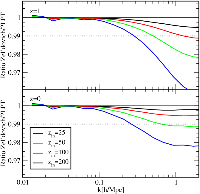
Figure 21: Comparison of the power spectra from simulations started from Zel’dovich initial conditions and 2LPT initial conditions at $z=1$ (upper panel) and $z=0$ (lower panel). Shown are the ratios of power spectra from starts at redshift $1+z_{\rm in}=200,100,50,25$. The start at $1+z_{\rm in}=200$ leads to an agreement of the power spectra better than 0.5% at $k\sim 1~{}h$Mpc^-1 and better than 0.2% at $z=0$. At larger scales, $k<0.1\,h\,{\rm Mpc}^{-1}$, the agreement is basically perfect. Therefore, the Zel’dovich initialization scheme started at $1+z_{\rm in}=200$ fulfills our accuracy requirements comfortably.

We generate four sets of initial conditions at $z_{\rm in}=200$, 100, 50 and 25. All of the initial conditions have the same phases and can therefore be compared directly. First, we measure the displacement from the Zel’dovich approximation; results are shown in the upper panel of Figure 18. For this one realization, the rms displacement at $z_{\rm in}=200$, which is the starting redshift for our main simulations, is around 5% of the mean interparicle spacing. By delaying the start until $z_{\rm in}=25$, the rms displacement grows by a factor of ten. The 2LPT correction, given by the second term in Eqn. (A1), is negligible at $z_{\rm in}=200$, being smaller than $10^{-4}$ on average. In fact at this point numerical accuracy might be questioned, since the approximations for the growth functions might not be accurate at this level. Figure 19 shows the ratio of the initial power spectra from the Zel’dovich and the 2LPT approximations. As for the displacements, convergence with increased redshift is very apparent. At a starting redshift of $z_{\rm in}=200$, both power spectra agree to better than 0.02%. Even starting at very late times ($z_{\rm in}=25$) only leads to a 1% difference between the initial power spectra.

Next we measure the differences in the initial velocities from the two approximations. The results are shown in Figure 20. We display the three velocity components $v_{x}$, $v_{y}$, and $v_{z}$ separately. The main difference occurs in the tails of the velocity distributions. Independent of redshift a negligible number of particles (fewer than 0.5%) live in these tails with absolute initial velocities larger than $1000\,$km/s. Ignoring these tails (see the insets in Figure 20), the difference in the velocities between 2LPT and ZA starting at different redshifts is below 1%. At $z_{\rm in}=200$ the difference is less than 0.1%. At this precision, the inaccuracy from the approximations for the growth function at first and second order is probably larger than the error from the Zel’dovich approximation.

The velocity differences are highly correlated with density however (see also Figure 5), and to understand this effect we evolve initial conditions created from the ZA and 2LPT forward to $z=0$. We use our parallel 2LPT code, which does not rely on an approximation for the growth function, to generate initial conditions with $512^{3}$ particles in a $468\,h^{-1}$Mpc box – downscaling our main runs by a factor of eight. The ICs are generated at four different redshifts, $1+z_{\rm in}=200$, 100, 50 and 25 and evolved to $z=0$ using a tree-PM code. We measure the power spectrum of the evolved particles at $z=1$ and $z=0$. The results are shown in Figure 21, where we see a shortfall in power at high $k$ in the ZA starts as compared to the 2LPT starts but convergence as $z_{\rm in}$ is increased. At $k\sim 1\,h\,{\rm Mpc}^{-1}$ the evolved power spectra from both sets of initial conditions at $1+z_{\rm in}=200$ show excellent agreement, better than 0.5% at $z=1$ and 0.25% at $z=0$. We therefore conclude that our starting redshift, $1+z_{\rm in}=200$, is high enough to avoid any problems arising from possible inadequacies of the Zel’dovich approximation.

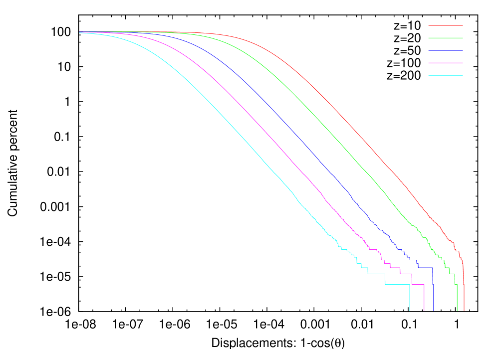
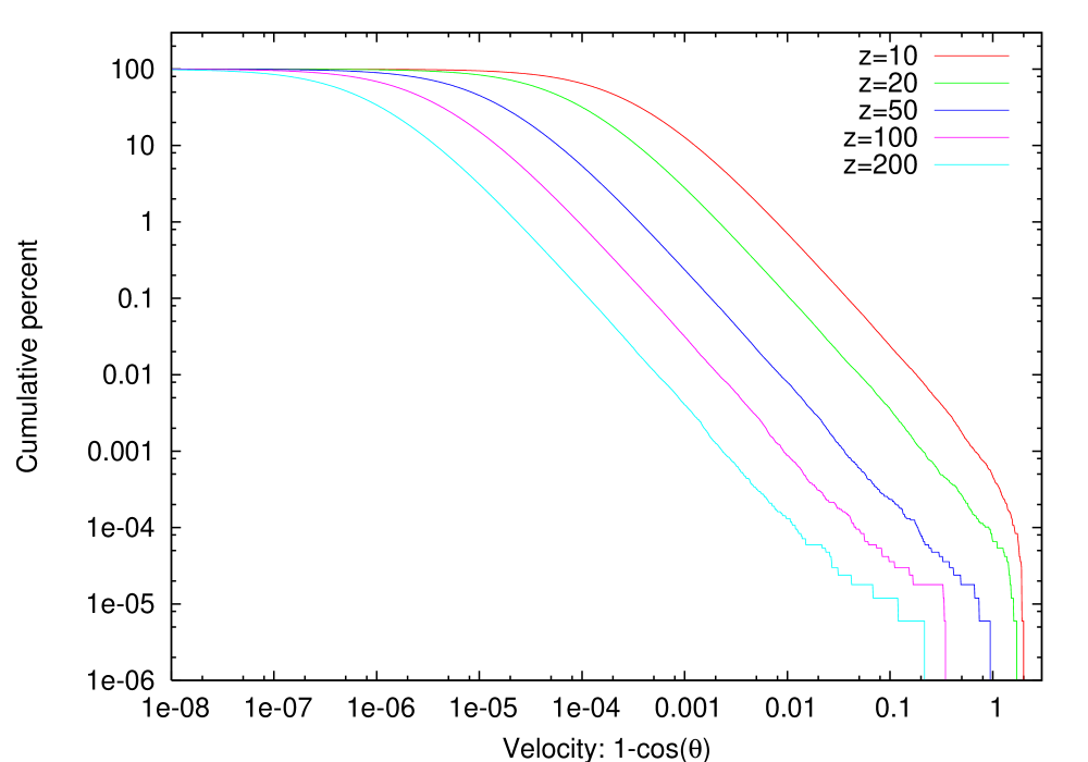
Figure 22: Cumulative distribution of the alignment angles $\cos(\theta)$ between the Zel’dovich and 2LPT displacement vectors (upper panel) and the velocity vectors (lower panel) at five different starting redshifts between $z=200$ and $z=10$. The test was carried out with 256³ particles in a $(1~{}h^{-1}$Gpc$)^{3}$ box. It is clear from these plots that the curvature in the path is a sub-dominant effect.

An argument as to why 2LPT might be preferable over the Zel’dovich approximation is that it can capture the displacement curvature, since it takes into account derivative terms (e.g., Bouchet et al. 1995, Fig. 1). In order to test this hypothesis we measure the distribution of misalignment angles: $\cos(\theta)$ between the Zel’dovich and 2LPT velocity and displacement vectors (Figure 22). When starting at high redshift ($z>50$) more than $\sim$99% of the particles have paths which differ in direction by less than about $1^{\circ}$. Hence the curvature in the path is a small effect for the vast majority of particles.

A more intuitive understanding of the difference between the Zel’dovich approximation and 2LPT (in part motivated by Fig. 5 of the velocity field around massive halos in different $z$-start simulations) is that 2LPT yields a slightly more convergent velocity toward regions of higher density. This slightly accelerates massive halo formation compared to the Zel’dovich approximation, resulting in the change in the mass function and power spectrum observed. This picture is supported by the fact that the most massive halos form about the largest density peaks where one might expect the assumption of small $\delta$ to hold the least well.

Appendix B Richardson Extrapolation

Richardson extrapolation is a method to compute the limiting value of a function that is assumed to have a smooth behavior for small deviations around the evaluation point. Suppose we have such a function $f$, then it is plausible to assume that

$$f(0+\Delta)=f(0)+c_{1}\Delta+c_{2}\Delta^{2}+c_{3}\Delta^{3}+\cdots.$$ (B1)

For many quantities derived from numerical simulations, it is not often a priori obvious what the convergence structure, i.e., the values of the coefficients, $c_{i}$, happens to be, even to the extent of knowing which of the coefficients are zero or non-zero. Nevertheless, for small enough values of the deviation, $\Delta$, one can numerically establish the values of the leading order coefficients. This allows one to bound the error from a given simulation, and could even (in principle) allow one to improve estimates for the desired limiting value $f(0)$ using Richardson extrapolation.

As a simple example, consider the case of non-zero $c_{1}$ (linear convergence) for some quantity, say the power spectrum at a given value of $k$, as a function of the mesh spacing in a PM code. Then, if we write, for a $256^{3}$ mesh,

$$f(2\Delta)\simeq f(0)+2c_{1}\Delta,\\$$ (B2)

for $512^{3}$ and $1024^{3}$ meshes we would have,

$$f(\Delta) \simeq f(0)+c_{1}\Delta,$$ (B3)

$$f\left(\frac{\Delta}{2}\right) \simeq f(0)+c_{1}\frac{\Delta}{2},$$ (B4)

where $\Delta$ has been taken to be the mesh spacing for the $512^{3}$ grid. Eqns. (B2) and (B3) then predict an estimated value for the 1024³ run

$$f\left(\frac{\Delta}{2}\right)\simeq\frac{3}{2}f(\Delta)-\frac{1}{2}f(2\Delta),$$ (B5)

which can be used to test whether linear convergence is holding for the particular range of values of $\Delta$. If the test is successful, one could then proceed to obtain an estimate for the continuum prediction ($\Delta=0$) from the 512³ and the 1024³ simulations, via

$$f(0)\simeq 2f\left(\frac{\Delta}{2}\right)-f(\Delta).$$ (B6)

We shall require simply that such a prediction differ from our highest resolution estimate by a negligible amount, to avoid explicit extrapolation.

For the case of quadratic convergence ($c_{1}=0$, $c_{2}\neq 0$), the extrapolation from the 256³ and the 512³ mesh to the 1024³ mesh reads:

$$f\left(\frac{\Delta^{2}}{4}\right)\simeq\frac{5}{4}f(\Delta^{2})-\frac{1}{4}f(4\Delta^{2}),$$ (B7)

and the estimate for the continuum from the 512³ simulation and the 1024³ simulation is given by:

$$f(0)\simeq\frac{4}{3}f\left(\frac{\Delta^{2}}{4}\right)-\frac{1}{3}f(\Delta^{2}).$$ (B8)

Given 3 simulations one can choose to estimate two non-zero coefficients, and test the assumed convergence model. As above, we shall require that such a prediction differ from our highest resolution estimate by a negligible amount, to avoid explicit extrapolation.

References

- Baugh et al. (1995) Baugh, C.M., Gaztanaga, E., & Estathiou, G., 1995, MNRAS, 274, 1049
- Benjamin et al. (2007) Benjamin J., et al., 2007, MNRAS, 381, 702
- Bernardeau et al. (2002) Bernardeau F., Colombi S., Gaztanaga E., Scoccimarro R., 2002, Phys. Rep. 367, 1
- Bouchet et al. (1995) Bouchet, F.R., Colombi, S., Hivon, E., & Juszkiewicz, R. 1995, A&A, 296, 575
- Carlson et al. (2009) Carlson J.W.G., White M., Padmanabhan N., 2009, Phys. Rev. D., in press [arxiv:0905.0479]
- Carroll et al. (1992) Carroll, S.M., Press, W.H., & Turner, E.L. 1992, Ann. Rev. Astron. Astrophys. 30 499
- Colombi et al. (2008) Colombi, S., Jaffe, A., Novikov, D., & Pichon, C., 2008, arXiv:0811.0313
- Cooray & Sheth (2002) Cooray, A. & Sheth, R. 2002, Phys. Rep., 372, 1
- Crocce et al. (2006) Crocce, M., Pueblas, S., & Scoccimarro, R. 2006, MNRAS 373, 369
- Dunkley et al. (2008) Dunkley, J. et al. 2008, arXiv:0803.0586
- Fu et al. (2008) Fu L., et al., 2008, A&A, 479, 9
- Gottlöber & Klypin (2008) Göttlober, S. & Klypin, A. 2008, in ”High Performance Computing in Science and Engineering Garching/Munich 2007”, Eds. Wagner, S.; Steinmetz, M.; Bode, A.; Brehm, M. Springer-Verlag 2008, p.29-43, arXiv:0803.4343
- Guillet, Teyssier & Colombi (2009) Guillet T., Teyssier R., Colombi S., 2009, submitted to A&A [arxiv:0905.2615]
- Habib et al. (2007) Habib, S., Heitmann, K., Higdon, D., Nakhleh, C., & Williams B. 2007, Phys. Rev. D, 76, 083503
- Hamilton et al. (1991) Hamilton, A.J.S., Kumar, P., Lu, E., & Matthews, A. 1991, ApJ, 3744, L1
- Haroz et al. (2008) Haroz, S., Liu, K.-W., & Heitmann, K. 2008, IEEE Pacific Visualization Symposium 2008, 4-7 March 2008, Kyoto, Japan; p.207-14 arxiv:0801.2405
- Haroz & Heitmann (2008) Haroz, S. & Heitmann, K. 2008, IEEE Computer Graphics and Applications, 28, 37
- Heitmann et al. (2005) Heitmann, K., Ricker, P.M., Warren, M.W. & Habib, S. 2005, ApJS, 28, 160.
- Heitmann et al. (2006) Heitmann, K., Higdon, D., Nakhleh, C., & Habib, S. 2006, ApJ 646, L1
- Heitmann et al. (2007) Heitmann, K. et al. 2008, Computational Science and Discovery, 1, 015003
- Heitmann et al. (2009) Heitmann, K., Higdon, D., White, M., Habib, S., Williams, B.J., Lawrence, E, & Wagner, C. 2009, ApJ (to appear)
- Hilbert et al. (2008) Hilbert, S., Hartlap, J., White, S.D.M., & Schneider, P. 2008, arXiv:0809.5035
- Hockney & Eastwood (1989) Hockney, R.W. & Eastwood, J.W., “Computer Simulation Using Particles”, Publ.: Taylor & Francis (1989)
- Hu & White (1997) Hu, W. & White, M. 1997, Phys. Rev. D, 56, 596
- Hu et al. (1998) Hu, W., Seljak, U., White, M., & Zaldarriaga, M. 1998, Phys. Rev. D, 57, 3290
- Huterer & Takada (2005) Huterer, D. & Takada, M. 2005, Astroparticle Phys. 23, 369
- Jarvis et al. (2006) Jarvis, M., Jain, B., Bernstein, G., and Dolney, D. 2006, ApJ 644, 71
- Jeong & Komatsu (2006) Jeong, D. & Komatsu, E. 2006, ApJ, 651, 619
- Jing et al. (2006) Jing, Y.P., Zhang, P., Lin W.P., Gao L., & Springel, V. 2006, ApJ 640, L119
- Joyce et al. (2008) Joyce, M., Marcos, B., & Baertschiger, T., arXiv:0805.1357v1
- Kilbinger et al. (2008) Kilbinger, M. et al., arXiv:0810.5129
- Kravtsov et al. (1997) Kravtsov, A.V., Klypin, A.A., & Khokhlov, A. M. 1997, ApJS 111, 73
- Lawrence et al. (2009) Lawrence, E., White, M., Higdon, D., Wagner, C., Heitmann, K., Habib, S., & Williams, B.J. 2009 (in preparation) ‘
- Lukić et al. (2007) Lukić, Z., Heitmann, K., Habib, S., Bashinsky, S., & Ricker, P.M. 2007, ApJ 671, 1160
- Ma (2007) Ma, Z. 2007, ApJ, 665, 887
- Massey et al. (2007) Massey R., et al., 2007, 172, 239
- Nishimichi et al. (2008) Nishimichi, T. et al., arXiv:0810.0813
- Peacock (1999) Peacock, J.A., “Cosmological Physics”, Pub.: Cambridge University Press (1999)
- Peacock & Dodds (1996) Peacock, J.A. & Dodds, S.J. 1996, MNRAS, 280, L19
- Rudd et al. (2008) Rudd, D.H., Zentner, A.R., & Kravtsov, A.V. 2008, ApJ, 672, 19
- Schneider et al. (2008) Schneider, M., Knox, L., Habib, S., Heitmann, K., Higdon, D., & Nakhleh, C., 2008, Phys. Rev. D, 78, 063529
- Scoccimarro (1998) Scoccimarro, R. 1998, MNRAS 299, 1097
- Seljak et al. (2003) Seljak, U., Sugiyama, N., White, M., & Zaldarriaga, M. 2003, Phys. Rev. D, 68, 083507
- Smith et al. (2003) Smith, R.E. et al. [The Virgo Consortium Collaboration], 2003, MNRAS 341, 1311
- Smith et al. (2007) Smith, R.E., Scoccimarro, R., & Sheth, R.K. 2007, Phys. Rev. D, 75, 063512
- Smith et al. (2008) Smith, R.E., Scoccimarro, R., & Sheth, R.K. 2008, Phys. Rev. D, 77, 043525
- Springel (2005) Springel, V., 2005, MNRAS 364 1105.
- Tang et al. (2008) While there are a large number of “forecast” papers, this is one of the most recent: Tang, J., Abdalla, F.B., and Weller, J., arXiv:0807.3140 [astro-ph].
- Takahashi et al. (2008) Takahashi, R., Yoshida, N., Matsubara, T., Sugiyama, N., Kayo, I., Nishimichi, T., Shirata, A., Taruya, A., Saito, S., Yahata, K., & Suto Y. 2008, MNRAS, 389, 1675
- White & Scott (1996) White, M. & Scott, D. 1996, ApJ, 459, 415
- White (2002) White, M. 2002, ApJS, 143, 241
- White (2004) White, M. 2004, Astropart. Phys. 22, 211
- Wong et al. (2008) Wong W.Y., Moss A., Scott D., 2008, MNRAS, 386, 1023
- Zel’dovich (1970) Zel’dovich, Y.B. 1970, A&A, 5, 84
- Zhan & Knox (2004) Zhan, H. & Knox, L. 2004, ApJ, 616, L75