Phenomenology of One-Dimensional Quantum Liquids Beyond the Low-Energy Limit

Abstract

We consider zero temperature behavior of dynamic response functions of 1D systems near edges of support in momentum-energy plane $(k,\omega).$ The description of the singularities of dynamic response functions near an edge $\varepsilon(k)$ is given by the effective Hamiltonian of a mobile impurity moving in a Luttinger liquid. For Galilean-invariant systems, we relate the parameters of such an effective Hamiltonian to the properties of the function $\varepsilon(k).$ This allows us to express the exponents which characterize singular response functions of spinless bosonic or fermionic liquids in terms of $\varepsilon(k)$ and Luttinger liquid parameters for any $k.$ For an antiferromagnetic Heisenberg spin$-1/2$ chain in a zero magnetic field, $SU(2)$ invariance fixes the exponents from purely phenomenological considerations.

One of the central problems in condensed matter theory is the development of an effective phenomenological description of complicated many-body systems, the microscopic details of which are often not known. The description of low energy properties of interacting electrons in normal metals, for example, is provided by the theory of Fermi liquid Nozieres , while in one-dimensional systems Luttinger liquid (LL) theory Haldane ; Giamarchibook ; GNT plays a similar role. These phenomenological theories do not rely on specific microscopic details, but predict certain low energy properties of many-body systems in terms of few measurable parameters. For example, LL theory assumes a linear spectrum of low energy excitations, and relates long-range behavior of correlation functions to the dimensionless LL parameter $K.$ However, the linear spectrum approximation is not sufficient for finding dynamic response functions (DRFs) even in low energy limit universal . In this Letter we show, that for a wide class of 1D systems one can phenomenologically predict certain properties of DRFs in terms of other measurable quantities even beyond the low energy limit.

The nonlinearity of the excitation spectrum affects transport phenomena, such as Coulomb drag drag and momentum-resolved tunneling of electrons Yacoby_science between quantum wires. In addition, neutron scattering on spin chains NS , ARPES on quasi-1D materials ARPES , and photoemission spectroscopy photo_Jin of 1D ultracold atomic gases directly measure DRFs, and are not limited to low energies. Evaluation of DRFs of 1D quantum systems with generic excitation spectrum is also a test bed for rapidly developing methods of numerical simulations of many-body dynamics DMRG ; Affleck2007 . Recently some progress was achieved in the analytical treatment of correlation functions beyond linear spectrum approximation universal ; Affleck2007 ; Pustilnik2006Fermions ; Khodas2006Fermions ; Pereira_bosons ; ImambekovGlazman_PRL ; CheianovPustilnik ; ZCG ; Arikawa ; Carmelo ; PustilnikCS ; KG ; bratskayamogila . The majority of analytical work however relied on solutions of microscopic models, using perturbation theory methods Pustilnik2006Fermions ; Khodas2006Fermions or integrability of models with specially tuned parameters Affleck2007 ; Pereira_bosons ; ImambekovGlazman_PRL ; CheianovPustilnik ; ZCG ; Arikawa ; Carmelo ; PustilnikCS . In contrast, the phenomenology developed in this Letter does not require any special property of the underlying microscopic interaction, while it provides relations between different experimentally observable quantities, such as the energy spectrum and the exponents of DRF singularities; see Eqs. (9) and (12).

For spinless fermionic Galilean-invariant systems, the DRFs have a sharp edge of support $\varepsilon(k)$ in the thermodynamic limit at $T=0;$ see Fig. 1. Hamiltonian describing singularities of DRFs, such as dynamic structure factor (DSF) $S(p,\omega)$ and spectral function $A(p,\omega)$ [defined below by Eqs. (1)-(2)], is the effective Hamiltonian of a mobile impurity moving in a LL Affleck2007 ; Pustilnik2006Fermions ; Khodas2006Fermions ; impurity ; Balents2000 ; see Eqs. (3)-(5) below. Singularities of DRFs at the edges of support are the main subject of this Letter. We show that their exponents for Galilean-invariant systems with interactions decaying faster than $\propto 1/x$ can be expressed as functions of $\varepsilon(k)$ and LL parameters. Phenomenological considerations allow us also to resolve the discrepancy Affleck2007 ; CheianovPustilnik regarding antiferromagnetic spin$-1/2$ XXZ model in zero magnetic field in favor of Ref. Affleck2007 .

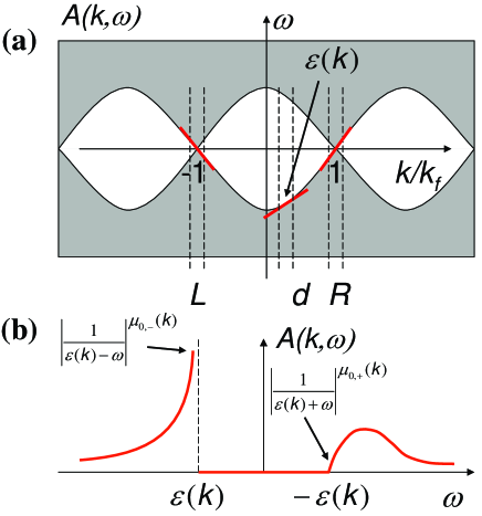
Figure 1: (Color online) (a) Spectral function $A(k,\omega)$ for spinless fermions in momentum-energy plane at $T=0.$ Shaded areas indicate the regions where $A(k,\omega)\neq 0,$ and $\varepsilon(k)$ is the edge of the support in the basic region $|k|<k_{f},\omega<0,$ where $k_{f}$ is Fermi momentum. Edges in other regions can be obtained from $\varepsilon(k)$ by combinations of shifts and inversions. (b) A sketch of constant $k$ scan of the spectral function for $|k|<k_{f}.$ Singularity of $A(k,\omega)$ near $\omega\approx\varepsilon(k)$ can be described using three-subband model of a mobile impurity moving in a Luttinger liquid, Eqs. (3)-(6), and the answer is given by Eqs. (9),(12).

We are interested in the zero temperature DSF

$$S(k,\omega)=\int\!dx\,dt\,e^{i(\omega t-kx)}\,\bigl{\langle}\rho(x,t)\rho(0,0)\bigr{\rangle},$$ (1)

and spectral function $A(k,\omega)=-\frac{1}{\pi}{\rm Im}G(k,\omega)\,{\rm sign}\omega,$ where Green’s function $G(k,\omega)$ is defined by AGD

$$G(k,\omega)=-i\int\int dxdte^{i(\omega t-kx)}\bigl{\langle}T\left(\Psi(x,t)\Psi^{\dagger}(0,0)\right)\bigr{\rangle}.$$ (2)

Here $\Psi(x,t)$ and $\rho(x,t)$ are annihilation and density operators, respectively, and $T$ denotes time ordering. Energy $\omega$ is measured from chemical potential, so $A(k,\omega)$ for $\omega>0\;(\omega<0)$ describes the response of the system to an addition of an extra particle (hole).

To be specific, we first discuss singularities of fermionic spectral function in the region $|k|<k_{f},\omega<0,$ where $k_{f}$ is Fermi momentum. Singularity can be described Pustilnik2006Fermions ; Khodas2006Fermions ; Affleck2007 by the effective Hamiltonian

$$H_{0}=\frac{v}{2\pi}\int dx\;\left[K(\nabla\theta)^{2}+\frac{1}{K}(\nabla\phi)^{2}\right],$$ (3)

$$H_{d}=\int dx\;d^{\dagger}(x)\left[\varepsilon(k)-iv_{d}\frac{\partial}{\partial x}\right]d(x),$$ (4)

$$H_{int}=\int dx\left[V_{R}\rho_{R}(x)+V_{L}\rho_{L}(x)\right]\rho_{d}(x)$$

$$=\int dx\left(V_{R}\nabla\frac{\theta-\phi}{2\pi}-V_{L}\nabla\frac{\theta+\phi}{2\pi}\right)d(x)d^{\dagger}(x).$$ (5)

Here $v$ is the sound velocity, and fields $\theta$ and $\phi$ describe low energy excitations and have a commutation relation $[\phi(x),\nabla\theta(x^{\prime})]=i\pi\delta(x-x^{\prime})$ (we use the notation of Ref. Giamarchibook ). Operator $d(x)$ creates a mobile hole of momentum $k$ and velocity $v_{d}=\partial\varepsilon(k)/\partial k,$ and operator $\rho_{d}(x)=d(x)d^{\dagger}(x)$ is the hole density. In terms of hole operator $d(x,t),$ The singular part of the spectral function near $\varepsilon(k)$ is given by

$$A(k,\omega)\propto\int dxdte^{i\omega t}\langle d^{\dagger}(x,t)d(0,0)\rangle_{H_{0}+H_{d}+H_{int}}.$$ (6)

Canonical transformation $\phi=\tilde{\phi}\sqrt{K},\theta=\tilde{\theta}/\sqrt{K}$ diagonalizes $H_{0},$ while the term $H_{int}$ can be removed Balents2000 by unitary transformation $U^{\dagger}(H_{0}+H_{d}+H_{int})U,$ where

$$U^{\dagger}=e^{-i\int dx\left\{\frac{\delta_{+}(k)}{2\pi}[\tilde{\theta}(x)-\tilde{\phi}(x)]-\frac{\delta_{-}(k)}{2\pi}[\tilde{\phi}(x)+\tilde{\theta}(x)]\right\}d(x)d^{\dagger}(x)}.$$

Momentum dependent phase shifts $\delta_{+}(k),\delta_{-}(k)$ are related to the parameters of $H_{int}$ as

$$\left(V_{L}-V_{R}\right)/\sqrt{K}=-\delta_{-}(k)(v_{d}+v)+\delta_{+}(k)(v_{d}-v),$$ (7)

$$\left(V_{L}+V_{R}\right)\sqrt{K}=-\delta_{-}(k)(v_{d}+v)-\delta_{+}(k)(v_{d}-v).$$ (8)

Calculating $U^{\dagger}d(x)U$ together with Eq. (6), one obtains

$$A(k,\omega)\propto\theta(\varepsilon(k)-\omega)\left|\frac{1}{\varepsilon(k)-\omega}\right|^{1-\left[\frac{\delta_{+}(k)}{2\pi}\right]^{2}-\left[\frac{\delta_{-}(k)}{2\pi}\right]^{2}}.$$ (9)

To obtain phase shifts, one needs to fix $V_{R}$ and $V_{L}$ in Eq. (5). We relate $V_{R}$ and $V_{L}$ to $\varepsilon(k)$ by calculating in two ways the shift of the position of the edge under uniform density and current variations.

Uniform density variation $\delta\rho$ results in a finite expectation value $\langle\nabla\varphi\rangle=-\pi\delta\rho.$ Evaluating the shift of $\varepsilon(k)$ in two ways, we obtain

$$-\frac{V_{R}+V_{L}}{2}=\frac{\partial\varepsilon(k)}{\partial\rho}+\frac{\partial\mu}{\partial\rho}=\frac{\partial\varepsilon(k)}{\partial\rho}+\frac{v\pi}{K}.$$ (10)

The left-hand side follows from the effective Hamiltonian given by Eqs. (3)-(5), while the right-hand side follows from the evaluation of the edge position from its thermodynamic definition [taking into account that energy $\varepsilon(k)$ is measured with respect to chemical potential $\mu$].

Uniform current through the system results in a finite value of $\langle\nabla\theta\rangle,$ which for Galilean-invariant systems corresponds to a motion with constant velocity $u=\langle\nabla\theta\rangle/m,$ where $m$ is the bare mass of the constituent particles. Then following the argument of Refs. Baym ; KG , one can use Galilean invariance to evaluate the change of $\varepsilon(k).$ Comparing it with the change evaluated using Eqs. (3)-(5) leads to

$$\frac{V_{L}-V_{R}}{2\pi}=\frac{k}{m}-\frac{\partial\varepsilon(k)}{\partial k}.$$ (11)

Combining now Eqs. (7) and (8) with Eqs. (10) and (11), we obtain the central result of this Letter

$$\frac{\delta_{\pm}(k)}{2\pi}=\frac{\frac{1}{\sqrt{K}}\left(\frac{k}{m}-\frac{\partial\varepsilon(k)}{\partial k}\right)\pm\sqrt{K}\left(\frac{1}{\pi}\frac{\partial\varepsilon(k)}{\partial\rho}+\frac{v}{K}\right)}{2\left(\pm\frac{\partial\varepsilon(k)}{\partial k}-v\right)}.$$ (12)

On the basis of Galilean invariance, it establishes a model-independent phenomenological relation between the edge position $\varepsilon(k)$ and other measurable quantities, such as the exponent of spectral function, Eq. (9). Even for usual LL theory Galilean-invariant systems are special. For them, LL parameter $K$ can be expressed Haldane as a renormalization of sound velocity compared to Fermi velocity $v_{f}$ in the absence of interactions, $K=v_{f}/v=\pi\rho/(mv).$ Our results are a generalization of the special properties of Galilean systems beyond low energy limit.

While Eq. (11) doesn’t hold on a lattice, Eq. (10) still works, and will be used below for the XXZ model. One can formulate an analog of Eq. (11) for LLs on lattices using the derivative of $\varepsilon(k)$ with respect to total flux through the system under periodic boundary conditions. Energies are easier to evaluate numerically than correlation functions, so our results can be used as a benchmark for numerical methods for evaluation of DRFs.

Away from the basic region $|k|<k_{f},\omega<0,$ positions of edges can be obtained from $\varepsilon(k)$ in the basic region by a combination of inversions and shifts. States which define the positions of the edges are given by a hole and excitations near Fermi points. Exponents of divergences can also be obtained using the three-subband model given by Eqs. (3)-(5), and here we only summarize the results.

For the spectral function momentum $k$ in the region $(2n-1)k_{f}<k<(2n+1)k_{f},$ hole momentum equals $k_{n}=k-2nk_{f}.$ Near the edges for $\omega>0(\omega<0),$ the spectral function is defined by

$$A(k,\omega)\propto\theta(\varepsilon(k_{n})\pm\omega)\left|\frac{1}{\omega\pm\varepsilon(k_{n})}\right|^{\mu_{n,\pm}(k)},$$ (13)

$$\mu_{n,\pm}(k)=1-\frac{1}{2}\left(2n\sqrt{K}-\frac{\delta_{+}(k_{n})+\delta_{-}(k_{n})}{2\pi}\right)^{2}$$

$$-\frac{1}{2}\left(\frac{1\pm 1}{\sqrt{K}}+\frac{\delta_{+}(k_{n})-\delta_{-}(k_{n})}{2\pi}\right)^{2}.$$ (14)

DSF $S(k,\omega)$ is non-vanishing only for $\omega>0,$ and for $2nk_{f}<k<2(n+1)k_{f}$ hole momentum is given by $k_{n}^{*}=(2n+1)k_{f}-k.$ The exponent of DSF $\mu_{n}(k)$ is defined by

$$S(k,\omega)\propto\theta(\omega+\varepsilon(k^{*}_{n}))\left|\frac{1}{\omega+\varepsilon(k^{*}_{n})}\right|^{\mu_{n}(k)},$$ (15)

$$\mu_{n}(k)=1-\frac{1}{2}\left[(2n+1)\sqrt{K}+\frac{\delta_{+}(k^{*}_{n})+\delta_{-}(k^{*}_{n})}{2\pi}\right]^{2}$$

$$-\frac{1}{2}\left(\frac{1}{\sqrt{K}}+\frac{\delta_{+}(k^{*}_{n})-\delta_{-}(k^{*}_{n})}{2\pi}\right)^{2}.$$ (16)

For bosons, spectral function has divergences at $\mp\varepsilon(k^{*}_{n})$ for $\omega>0(\omega<0),$ and exponents equal

$$\mu^{b}_{n,\pm}(k)=1-\frac{1}{2}\left[(2n+1)\sqrt{K}-\frac{\delta_{+}(k^{*}_{n})+\delta_{-}(k^{*}_{n})}{2\pi}\right]^{2}$$

$$-\frac{1}{2}\left(\frac{1\pm 1}{\sqrt{K}}+\frac{\delta_{+}(k^{*}_{n})-\delta_{-}(k^{*}_{n})}{2\pi}\right)^{2}.\;\;$$ (17)

Let us now discuss several cases where one can explicitly check our phenomenological predictions. The shift of the position of $\varepsilon(k)$ can be evaluated using perturbation theory in interaction strength for any momenta, and predictions following from our theory coincide with results of Refs.  Pustilnik2006Fermions ; Khodas2006Fermions . By using approximation $\varepsilon(k)\approx v(k-k_{f})$ for any interaction strength in the vicinity of the right Fermi point, from Eqs. (8) and (10) one can recover the universal phase shift  universal

$$\frac{\delta_{-}(k_{f}-0)}{2\pi}=\frac{1}{2\sqrt{K}}-\frac{\sqrt{K}}{2},$$ (18)

which holds irrespective of Galilean invariance. One can also obtain $\delta_{+}(k_{f}-0)$ from Eq. (12). For that, one has to use the expansion $\varepsilon(k)\approx v(k-k_{f})+(k-k_{f})^{2}/(2m_{*}),$ and the expression for $1/m_{*}$ obtained in Ref. Pereira_bosons , which is valid for Hamiltonians with interactions decaying faster than $\propto 1/x^{2}.$ For Galilean-invariant systems, it simplifies to $1/m_{*}=[\sqrt{K}/(2\pi)]\partial{v}/\partial{n}+1/(2m\sqrt{K}),$ and after some simple algebra with Eq. (12) one reproduces universal phase shift universal $\delta_{+}(k_{f}-0)/(2\pi)=1-1/(2\sqrt{K})-\sqrt{K}/2.$ One can also explicitly check, that exponents for Lieb-Liniger Lieb and Calogero-Sutherland BM models evaluated from their excitation spectra reproduce the results of Refs. ImambekovGlazman_PRL and  Khodas2006Fermions ; PustilnikCS , respectively.

The crucial step in the calculation of the exponents is the identification of the spectral function $A(k,\omega)$ defined in terms of constituent particles, Eq. (2), with the correlation function of operator $d$ in Eq. (6). Comparison with solvable cases above shows that such identification indeed holds in the vicinity of Fermi points for any interactions, as well as for any momentum for weak interactions. While we cannot prove that it holds for any strongly interacting Galilean-invariant system, we expect it to be valid as long as the position of the edge satisfies

$$\left|\frac{\partial\varepsilon(k)}{\partial k}\right|<v\;\;\mbox{for}\;|k|<k_{f},$$ (19)

and interactions decay faster than $\propto 1/x.$ Equation (19) guarantees that phases in Eq. (12) are continuous functions of momentum, and the state which corresponds to the edge of the basic region of the spectral function support does not contain particle-hole excitations near left or right Fermi points.

Let us now discuss how considerations of this Letter can resolve a discrepancy between results of Refs. Affleck2007 and CheianovPustilnik for correlations of the XXZ model in zero magnetic field. In our notations, these references predict $\delta^{PWA}_{-}(k)/(2\pi)=-\delta^{PWA}_{+}(k)/(2\pi)=(1/\sqrt{K}-\sqrt{K})/2$ and $\delta^{CP}_{-}(k)/(2\pi)=-\delta^{CP}_{+}(k)/(2\pi)=(1-K)/2,$ respectively. Identification of these phase shifts was based on the analysis of finite size corrections to energies obtained from the exact solution. Their interpretation for the XXZ model in zero magnetic field is ambiguous, since the half-filled lattice is a special point for the Bethe Ansatz solution KBI . On the other hand, our approach constrains phase shift via $\varepsilon(k),$ which is well defined in the thermodynamic limit, and resolves the discrepancy.

First, we note that $\delta^{PWA}_{-}(k)$ satisfies universal relation given by Eq. (18), while $\delta^{CP}_{-}(k)$ does not. Second, Eqs. (7),(8) and (10) hold on the lattice for any $k,$ and one can easily evaluate excitation spectrum of the XXZ model numerically from the exact solution KBI . This way, we have verified that $\delta^{PWA}_{\pm}(k)$ satisfy them, while $\delta^{CP}_{\pm}(k)$ do not. Third, one can use $SU(2)$ invariance to independently derive results of Ref. Affleck2007 at the XXX point. The argument is very similar to the reasoning which fixes LL parameter $K=1/2$ at $XXX$ point Giamarchibook ; GNT by requiring that long distance asymptotes of $\langle S^{z}(x)S^{z}(0)\rangle$ and $\langle S^{-}(x)S^{+}(0)\rangle$ coincide. But $SU(2)$ symmetry also establishes a relation between spin DRFs $S^{zz}(k,\omega)$ and $S^{-+}(k,\omega)$ in entire momentum-energy plane, including the edges of supports. There $S^{zz}(k,\omega)$ behaves as the sum of different power laws (up to logarithmic corrections)

$$S^{zz}(k,\omega)\propto\sum_{l}\left|\frac{1}{\omega-\varepsilon(k)}\right|^{\mu^{zz}_{l}}.$$ (20)

Different power laws appear because of the umklapp processes that are allowed on a half-filled lattice. $SU(2)$ symmetry implies that the same set of exponents should apply for $S^{-+}(k,\omega)$ as well. These exponents can be evaluated in terms of $\delta_{\pm}(k)$ and $K$ for any $l,$ and the coincidence of two sets of exponents unambiguously fixes

$$\frac{\delta_{\pm}(k)}{2\pi}=\mp\frac{1}{2\sqrt{2}},$$ (21)

as in Ref. Affleck2007 for $K=1/2.$ Full sequence of exponents is

$$\mu^{zz}_{l}=3/4-(4l+1)^{2}/4.$$ (22)

Note, that we did not use integrability in the argument for the XXX model, so Eq. (22) should apply for $SU(2)$ invariant models with longer range interactions as well, if the spin chain remains a gapless LL.

To summarize, we have considered zero temperature dynamic response functions of 1D systems near edges of support in the momentum-energy plane. Continuous symmetries can be used to fix the exponents of power law divergences of dynamic response functions near the edges. For spinless Galilean-invariant systems of fermions or bosons, we have obtained phenomenological expressions, Eqs. (12),(14),(16), and (17), which establish model-independent relations of the exponents of dynamic response functions to the position of the edge of support $\varepsilon(k).$ For a spin$-1/2$ anitferromagnetic Heisenberg chain in zero magnetic field, $SU(2)$ symmetry dictates exponents given by Eq. (22) for all momenta regardless of the interaction range.

We thank A. Kamenev and A. Lamacraft for useful discussions, and NSF Grant DMR-0754613 for support.

References

- (1) P. Nozières, Theory of Interacting Fermi Systems (Addison-Wesley, Reading, MA, 1997).
- (2) F.D.M. Haldane, Phys. Rev. Lett. 47, 1840 (1981); J. Phys. C 14, 2585 (1981).
- (3) T. Giamarchi, Quantum Physics in One Dimension (Oxford University Press, New York, 2004).
- (4) A. Gogolin, A. Nersesyan, and A. Tsvelik, Bosonization and Strongly Correlated Systems (Cambridge University Press, Cambridge, England, 1998).
- (5) A. Imambekov and L.I. Glazman, Science 323, 228 (2009).
- (6) M. Pustilnik et al., Phys. Rev. Lett. 91, 126805 (2003); M. Yamamoto et al., Science 313, 204 (2006).
- (7) O.M. Auslaender et al., Science 295, 825 (2002).
- (8) B. Lake et al., Nature Mater. 4, 329 (2005).
- (9) B.J. Kim et al., Nature Phys. 2, 397 (2006).
- (10) J.T. Stewart, J.P. Gaebler, and D.S. Jin, Nature 454, 744 (2008).
- (11) S.R. White and I. Affleck, Phys. Rev. B 77, 134437 (2008); A.E. Feiguin and D. Huse, arXiv:0809.3024.
- (12) R. G. Pereira, S. R. White, and I. Affleck, Phys. Rev. Lett. 100, 027206 (2008).
- (13) M. Pustilnik et al., Phys. Rev. Lett. 96, 196405 (2006).
- (14) M. Khodas et al., Phys. Rev. B 76, 155402 (2007).
- (15) R.G. Pereira et al., Phys. Rev. Lett. 96, 257202 (2006); J. Stat. Mech. (2007) P08022.
- (16) A. Imambekov and L.I. Glazman, Phys. Rev. Lett. 100, 206805 (2008).
- (17) V.V. Cheianov and M. Pustilnik, Phys. Rev. Lett. 100, 126403 (2008).
- (18) M. B. Zvonarev, V. V. Cheianov, and T. Giamarchi, Phys. Rev. Lett. 99, 240404 (2007); arXiv:0811.2676.
- (19) T. Yamamoto et al., Phys. Rev. Lett. 84, 1308 (2000); M. Arikawa, Y. Saiga, and Y. Kuramoto, ibid. 86, 3096 (2001).
- (20) M. Pustilnik, Phys. Rev. Lett. 97, 036404 (2006).
- (21) J.M. Carmelo et al., Phys. Rev. Lett. 83, 3892 (1999); J.M.P. Carmelo, K. Penc, and D. Bozi, Nucl. Phys. B725, 421 (2005); J. Phys. Condens. Matter 20, 415103 (2008).
- (22) A. Kamenev, L.I. Glazman, arXiv:0808.0479v1.
- (23) M. Khodas et al., Phys. Rev. Lett. 99, 110405 (2007); K. A. Matveev and A. Furusaki, ibid. 101, 170403 (2008); A. V. Rozhkov, Phys. Rev. B 74, 245123 (2006); D. N. Aristov, ibid. 76, 085327 (2007); S. Akhanjee and Y. Tserkovnyak, ibid. 76, 140408 (2007); D. B. Gutman, ibid. 77, 035127 (2008); A.V. Rozhkov, ibid. 77, 125109 (2008); M. Khodas, A. Kamenev, L. I. Glazman, Phys. Rev. A 78, 053630 (2008).
- (24) T. Ogawa, A. Furusaki, and N. Nagaosa, Phys. Rev. Lett. 68, 3638 (1992); S. Sorella and A. Parola, ibid. 76, 4604 (1996); Phys. Rev. B 57 6444 (1998); A. Friedrich et al., ibid. 75, 094414 (2007); A. Lamacraft, arXiv:0810.4163.
- (25) L. Balents, Phys. Rev. B 61, 4429 (2000).
- (26) A.A. Abrikosov, L.P. Gorkov, and I.E. Dzyaloshinski, Methods of Quantum Field Theory in Statistical Physics, (Dover, New York, 1963).
- (27) G. Baym and C. Ebner, Phys. Rev. 164, 235 (1967).
- (28) E.H. Lieb and W. Liniger, Phys. Rev. 130, 1605 (1963); E.H. Lieb, ibid. 130, 1616 (1963).
- (29) B. Sutherland, Beautiful Models (World Scientific, Singapore, 2004).
- (30) V.E. Korepin, N.M. Bogoliubov, and A.G. Izergin, Quantum Inverse Scattering Method and Correlation Functions (Cambridge University Press, Cambridge, England, 1993).