Crossover transition in bag-like models

Abstract

We formulate a simple model for a gas of extended hadrons at zero chemical potential by taking inspiration from the compressible bag model. We show that a crossover transition qualitatively similar to lattice QCD can be reproduced by such a system by including some appropriate additional dynamics. Under certain conditions, at high temperature, the system consist of a finite number of infinitely extended bags, which occupy the entire space. In this situation the system behaves as an ideal gas of quarks and gluons.

I Introduction

The phase transition of strongly interacting matter has been intensively studied for many years. As early as 1960s, before the discovery of QCD, there was speculation about a possible new phase of strongly interacting matter, based on studies of the thermodynamics of a hadron gas. Particularly, in the Statistical Bootstrap Model Hagedorn:1972gv , the asymptotically exponential mass spectrum of hadrons implied the existence of a limiting temperature of about $170$ MeV (the Hagedorn temperature) above which hadrons cannot exist.

After the discovery of QCD and in particular asymptotic freedom, the discussion focused on the ideas of a Quark Gluon Plasma (QGP), a system of weakly interacting quarks and gluons, and a possible transition between a pion gas and a quark gluon plasma. The physical picture for such a transition was that at the critical temperature the additional degrees of freedom carried by the quarks and gluons would be released leading to a rapid increase of the entropy, energy-density and pressure. This was supported by first Lattice QCD (LQCD) calculations creutz . Lately, however, the hadron resonance gas experienced a renaissance mainly due to its successful description of hadron yields in heavy ion and also elementary particle collisions BraunMunzinger:1995bp ; Cleymans:1996cd ; Broniowski:2002nf ; Becattini:2005xt ; Andronic:2008gm ; Manninen:2008mg ; Becattini:1995if ; Becattini:1996gy ; Becattini:1997rv ; Becattini:2001fg . In addition it was realized that the sharp rise of the entropy density near the transition temperature, as observed in lattice QCD calculations, could be accounted for by a hadron resonance gas as well Karsch:2003vd ; Cheng:2007jq . The success of the hadron resonance gas below the transition temperature $T_{c}$, however, changes the physical interpretation for the QCD phase transition. Instead of releasing additional degrees of freedom at $T_{c}$, the system has to reduce the number of active degrees of freedom at the transition temperature, because a hadron gas has many more than a Quark Gluon plasma. In case of a Hagedorn exponential mass spectrum, the entropy density actually diverges at the Hagedorn temperature. But even if the number of hadrons is restricted to those needed for a successful description of hadronic final states in heavy ion and elementary particle collisions, the entropy quickly exceeds that observed on the lattice.

Meanwhile many papers have addressed this issue ranging from QCD-based approaches (see for example Karsch:2003vd ; Rischke:1987xe ; Mingmei:2007jx ) to various generalizations of the hadron gas Hagedorn:1980cv ; Rafelski:1980rk ; Kapusta:1981ay ; Gorenstein:1981fa ; Kagiyama:1992kt ; Gorenstein:1998am ; Kagiyama:2002rm ; Gorenstein:2005rc ; Zakout:2006zj ; Bugaev:2007ww ; Zakout:2007nb . In this article we will study the transition region, and we will provide a simple and intuitive modification to the hadron gas model in order to qualitatively reproduce the crossover transition observed in Lattice QCD Aoki:2006we . Our calculations are based on the ideas proposed in Gorenstein:1998am , where it was shown that under certain circumstances a gas of extended hadrons could produce phase transitions of the first or second order, and also a smooth crossover transition that might be qualitatively similar to that of lattice QCD.

We first observe that for the typical particle density at the transition the size of hadrons needs to be taken into account as it leads to a considerable suppression of the available phase space. As a result the number of effective degrees of freedom is reduced. This suppression alone, however, does not explain the ideal gas behavior of lattice QCD at high temperatures, above $T_{c}$. Additional model assumptions have to be made. For example one could explicitly introduce a deconfined phase and then match the two different phases. For this exercise to work, however, rather detailed assumptions about the intrinsic nature of hadrons have to be made in order to avoid the occurrence of an actual phase transition Mingmei:2007jx . In this paper, we follow a different route. We adopt the philosophy that the same partition function should describe both “phases”. To this end we need to introduce appropriate dynamics in order to model the crossover observed on the lattice. This approach is similar in spirit to Gorenstein:1998am . We find that the MIT bag model Chodos:1974je of the hadrons is well suited for our purposes, because it embodies confined and deconfined phases from the very beginning. Thus, we will describe hadrons as extended bags of QGP and we will assume an infinite mass spectrum of the Hagedorn’s type. The additional dynamics needed to describe the transition are simply the elastic interactions between hadrons. They give rise to a kinetic pressure that in turn “squeezes” the bag-like hadrons. We find that the behavior of our system depends sensitively on the choice of parameters for the mass spectrum. One can obtain either a real phase transition  Gorenstein:1981fa ; Gorenstein:1998am or, as we shall show, a crossover. In addition, in the latter case the specific parametrization for the mass spectrum affects the microscopic structure of the gas of “compressible” hadrons at high temperatures ($T>T_{c}$). One finds either a high temperature phase that is populated by one or few infinitely large bags, consistent with the usual picture of a QGP. Or, for a different choice of parameters, one obtains a system of many, densely packed heavy hadrons, which nonetheless exhibit the thermodynamic properties of a QGP of massless quarks and gluons.

On first sight, our approach appears to be similar to the ideas of percolation models percth1 ; Coniglio:1980zz ; Fortunato:1999wr ; Fortunato:2000ge ; Fortunato:2000hg ; Fortunato:2000vf . The finite size corrections to the statistical ensemble remove all the configurations with overlapping hadrons, resulting in large hadronic states dominating the partition function. This is similar to percolation. However, there are quite some differences in the specific implementation. First, in our model, we do not consider an explicit coupling between the bags as it is done in the percolation model of Fortunato:1999wr ; Fortunato:2000ge ; Fortunato:2000hg ; Fortunato:2000vf . Instead, we take the effect of the kinetic pressure onto the bag sizes into account, resulting in a self-consistency relation for the effective bag pressure. This is more in the spirit of a mean field description, although we do not introduce an additional interaction but simply consider the kinetic pressure. Second, in contrast to purely geometric percolation, in our model the number of hadrons and their sizes are not independent quantities. In a given multihadron state, melting two or more hadrons together (to form a bigger one) results in a different kinetic pressure and, in turn, in the rearrangement of the sizes of all the hadrons.

Throughout this paper, we will maintain a simple schematic approach to highlight the main features of the model leaving a more detailed quantitative analysis and further generalizations to future work. We will confine ourselves to the simplest case of nonrelativistic Boltzmann particles and we will neglect subtleties such as surface effects and van der Waals type residual interaction among the bags.

This paper is organized as follows: in Section II we introduce the main ideas of the model and derive the grand-canonical partition function for the gas of compressible hadrons. In Section III we will use the corresponding isobaric partition function to perform a comprehensive numerical analysis. We will study the pressure, the energy density and the entropy density of the system. We will further analyze particles number, the filling fraction and the average mass of particles in the system.

II The partition function

In this section we will set up the general formalism for our model. Let us start with the partition function $Z(V,T)$ of an ideal gas of Boltzmann particles of mass $m$ and degeneracy $g$ in the nonrelativistic limit. For the subsequent discussion it is advantageous to express the partition function $Z(V,T)$ in a multiplicity expansion, i.e. as a sum of partition functions $Z_{N}(V,T)$ for fixed particle numbers $N$:

$$Z(V,T)\equiv\sum_{N=0}^{\infty}Z_{N}(V,T)\equiv\sum_{N=0}^{\infty}\frac{1}{N!}\left(gV\right)^{N}\phi(m,T)^{N}\;,$$ (1)

with

$$\phi(m,T)\equiv\frac{1}{(2\pi)^{3}}\int{\rm d}^{3}{\rm p}\exp{\left[-\left(\frac{{\rm p}^{2}}{2mT}+\frac{m}{T}\right)\right]}=\exp{\left[-\frac{m}{T}\right]}\left(\frac{mT}{2\pi}\right)^{3/2}\;.$$ (2)

Here $V$ and $T$ are the volume and the temperature of the system, respectively. The function $Z$ is the grand-canonical partition function with vanishing chemical potentials. In the context of this paper we shall refer to $Z_{N}$ as the canonical partition function keeping in mind that this notation deviates from the conventions for relativistic hadron gases, where the canonical ensemble has fixed Abelian charges (such as electric charge, strangeness, baryon number), but no constraints on the number of particles. Eq. (1) can be easily generalized to a multispecies gas of particles. If we label with $j=1,\ldots,K$ the various particle species we have:

$$Z(V,T)=\prod_{j=1}^{K}\left[\sum_{N_{j}=0}^{\infty}\frac{1}{N_{j}!}\left(g_{j}V\right)^{N_{j}}\phi(m_{j},T)^{N_{j}}\right]=\exp{\left[V\sum_{j=1}^{K}g_{j}\phi(m_{j},T)\right]}\;.$$ (3)

In case of $K\rightarrow\infty$, it is convenient to replace the discrete index $j$ with a continuous spectrum density $\rho(m)$ so that the number of species in the mass interval $[m,m+{\rm d}m]$ is given by $\rho(m){\rm d}m$. Formally, we make the substitution:

$$\sum_{j=1}^{\infty}g_{j}\phi(m_{j},T)\rightarrow\int{\rm d}m\rho(m)\;\phi(m,T)\;.$$ (4)

By expanding the exponential in Eq. (3) the partition function can then be written as:

$$Z(V,T)=\sum_{N=0}^{\infty}\frac{V^{N}}{N!}\left[\prod_{i=1}^{N}\int_{0}^{\infty}{\rm d}m_{i}\rho(m_{i})\;\phi(m_{i},T)\right]\;.$$ (5)

Because a hadron gas, or, more precisely, a Hagedorn gas is characterized by an exponential mass spectrum, we set

$$\rho(m)=c_{0}\frac{\textrm{e}^{m/T_{0}}}{m^{\alpha}}\;,$$ (6)

where the parameters $c_{0}$ and $\alpha$ will be determined from empirical data. In the case of gas-of-bags models, which also have an exponential mass spectrum, the parameters $c_{0}$ and $\alpha$ will have to be determined from the underlying (dynamical) model parameters, such as bag pressure, and so on. We note that $c_{0}$ has dimensions of $[\rm mass]^{\alpha-1}$ and $\alpha$ typically ranges from $\alpha=0$ to $\alpha\sim 7$ depending on the model. In Eq. (6), $T_{0}$ simply parametrizes the mass spectrum. In the context of the MIT bag model, $T_{0}$ can be interpreted as the effective “temperature” inside the bag, as will be discussed in section II.1. By substituting Eq. (6) in Eq. (5) we arrive at the following partition function for a hadron gas

$$Z(V,T) = \sum_{N=0}^{\infty}\left(\frac{T}{2\pi}\right)^{3N/2}\frac{(Vc_{0})^{N}}{N!}\left[\prod_{i=1}^{N}\int_{0}^{\infty}{\rm d}m_{i}\;m_{i}^{3/2-\alpha}\right]$$

$$\times\exp{\left[\frac{\sum_{i=1}^{N}m_{i}}{T_{0}}-\frac{\sum_{i=1}^{N}m_{i}}{T}\right]}\;.$$

This partition function $Z(V,T)$ (and also $Z_{N}(V,T)$) is divergent for $T>T_{0}$ as already pointed out by Hagedorn. Although an upper limit in the mass spectrum $\rho(m)$ regulates the divergences, it will not prevent the system from having a much higher entropy density than that observed on the lattice.

An exponential mass spectrum without any cutoff may certainly be an oversimplification and a more realistic calculation may take into account discrete states as well as a mass spectrum that grows less than exponential above a certain mass. However, empirically the known hadronic states do indeed grow exponentially up to a mass of $m\sim 2\,\rm GeV$. Above that, very few states are known and it is not clear if this is an indication of a saturating density of states or simply the lack of experimental data on higher mass resonances. Therefore, working with an exponential mass spectrum without any cutoff appears to be an approximation as good as any other. Furthermore, because we are interested only in bulk thermodynamic quantities such as energy density and pressure, the use of a continuous mass spectrum should be a reasonable approximation as all these quantities represent integrals/sums over the mass spectrum. Therefore, in this paper we will assume that the mass spectrum is of the Hagedorn type and will discuss a dynamical scenario in the framework of the MIT bag model, which will regulate the partition function.

II.1 The regularized partition function

To develop the partition function of our model, we need to recall some of the basic features of the MIT bag model Chodos:1974je . In its simplest formulation, hadrons can be considered as bags of partonic fields confined in a spatial region with a constant potential energy per unit volume $B$, where $B$ is commonly referred as the bag constant or bag pressure. The total energy, i.e. the mass $m$ of a bag with volume $V_{b}$ is then given by Chodos:1974je :

$$m=U+BV_{b}\;,$$ (8)

where $U$ is the internal energy of the field inside the bag. When its linear extension is larger than the wavelengths of the partons (the quanta of the inner field), we can approximate the bag by a gas of free massless particles confined to its volume Chodos:1974je . For a sufficiently large $V_{b}$, the internal energy is then given by the relation:

$$U=3p_{r}V_{b}\;,$$ (9)

where $p_{r}$ is the pressure of the gas. For a single hadron the stability condition requires:

$$p_{r}\equiv B\;,$$ (10)

which then gives

$$m=4BV_{b}\;.$$ (11)

The effective temperature of the bag is related to the bag pressure by the relation $T_{0}\equiv kB^{1/4}$, where $k$ is a dimensionless constant whose value depends on the number of internal degrees of freedom of the gas inside the bag. For large $V_{b}$, the entropy $S$ of a bag, is the entropy of a massless gas with internal energy $U$ and pressure $B$ Chodos:1974je , therefore,

$$S=\frac{4U}{3kB^{1/4}}\equiv\frac{4U}{3T_{0}}=\frac{m}{T_{0}}\;.$$ (12)

From Eq. (12) one can derive the level density

$$\rho(m)\propto\textrm{e}^{S}\propto\textrm{e}^{m/T_{0}}\;.$$ (13)

Note that the generic spectrum introduced in Eq. (6), has an additional contribution: $m^{-\alpha}$. This factor can be interpreted as a logarithmic correction to the entropy of the bag. In what follows, we will retain the spectrum in Eq. (6) and we will analyze different values of $\alpha$. Of course, Eq. (13) will correspond to the case $\alpha=0$.

Once the temperature $T$ of the gas of bags approaches $T_{0}$, the average masses and hence the volume (see Eq. (11)) of the bags grow very fast. Therefore, the bag-like hadrons tend to occupy more and more of the available space and, eventually, they will overlap. To avoid multiple counting of the phase space, configurations with overlapping bags need to be excluded from the partition function. For a finite system of volume $V$ this can be achieved with an excluded volume correction, where the total volume $V$ is replaced by the available volume $(V-\sum_{i=1}^{N}V_{i})^{N}$, where $V_{i}$ is the volume of the $i-$th particle. In addition the volume of all bags $\sum_{i=1}^{N}V_{i}$ should not exceed the total volume $V$. Following Ref. Gorenstein:1981fa , this leads to the modified $N$-particle phase space integral

$$\left[\prod_{i=1}^{N}\frac{V}{(2\pi)^{3}}\int{\rm d}^{3}{\rm p}\right]\rightarrow\left[\prod_{i=1}^{N}\frac{1}{(2\pi)^{3}}\int{\rm d}^{3}{\rm p}\right]\left(V-\sum_{i=1}^{N}V_{i}\right)^{N}\Theta{\left(V-\sum_{i=1}^{N}V_{i}\right)}\;.$$ (14)

This modified phase space integral results in a well-defined and finite partition function at every temperature

$$Z(V,T)=\sum_{N=0}^{\infty}\left(\frac{T}{2\pi}\right)^{3N/2}\frac{c_{0}^{N}}{N!}\left[\prod_{i=1}^{N}\int_{0}^{\infty}{\rm d}m_{i}\;m_{i}^{3/2-\alpha}\right]$$ (15)

$$\times\exp{\left[\frac{\sum_{i=1}^{N}m_{i}}{T_{0}}-\frac{\sum_{i=1}^{N}m_{i}}{T}\right]}\left(V-\sum_{i=1}^{N}V_{i}\right)^{N}\Theta{\left(V-\sum_{i=1}^{N}V_{i}\right)}\;.$$

It can be shown that such a system of extended hadrons leads to a constant value for the energy-density $\varepsilon$, in contradiction with Lattice QCD, where the energy density is found to increase with the fourth power of the temperature, $\epsilon_{\rm Lattice}\sim T^{4}$. In fact, for $T\rightarrow\infty$, the most favorite configurations are those where the hadrons occupy all the available space. In this case, the energy density of the system correspond to $\varepsilon=4B$, i.e. the inner density of the hadrons (see Eq. (11)). The underlying reason for this behavior is that the system is not able to pick up additional kinetic energy once the entire volume is filled with bags, as the bags have no more room to move.

Obviously some additional dynamics needs to be included to allow for the system to pick up more energy as the temperature is increased. To this end we adopt the idea of compressible bags Kagiyama:2002rm . More precisely, we will allow the volume of the hadrons to vary under the effect of the pressure generated by their own thermal motion in a self-consistent way. Consequently, as the temperature and hence the pressure increase, the bags will be compressed and acquire a higher internal mass/energy density. We will show that the system does not exhibit any limiting value of the energy density, and, under appropriate conditions, exhibits the desired increase of the energy density and entropy.

To illustrate the underlying mechanism, let us consider a gas of many hadrons. For small temperatures, $T\ll T_{0}$, the system is dilute ($V\gg\sum_{i=1}V_{i}$) and behaves like a gas of noninteracting point-particles. With increasing temperature, the average mass, and hence the spatial extent of the hadrons, increases and as $T$ approaches $T_{0}$ the dilute-gas approximation seizes to be valid. The pressure exerted by the other particles becomes sizable and its effect on the hadrons properties, such as the size, can no longer be ignored. In other words, in addition to the bag pressure $B$, every particle in the system will feel an additional kinetic pressure $p_{k}$ that is generated by the thermal motion of the other hadrons in the gas. In this situation, the stability condition, Eq. (10), needs to be modified by taking onto account the contribution of the kinetic pressure $p_{k}$. Microscopically, the pressure $p_{k}$ can be interpreted as the consequence of elastic collisions. The effect of inelastic collisions, which are certainly present in a hadron gas, in our approach are accounted by the infinite mass spectrum of hadrons without enforcing any constraint on the number of particles $N$. In this way all the possible configurations with few large hadrons or many small ones are included. This is analogous to the hadron-resonance gas model, where a large part of the inelastic interaction is taken into account by adding resonances as free particles in the gas.

Neglecting any surface effect, the simplest generalization of the stability condition, Eq. (10), is

$$p_{r}=B+p_{k}(V,T)\;.$$ (16)

A pictorial illustration of the pressure balance in the last equation is given in Fig. (1).

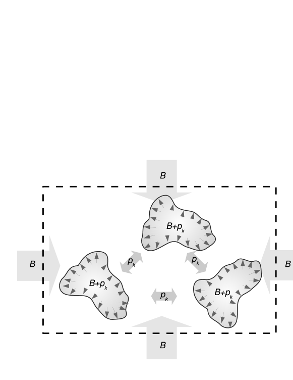
Figure 1: Pictorial representation of the pressure balance in a gas of compressible hadrons. The internal hadron pressure must be equal to the sum of the constant bag pressure $B$ plus the pressure $p_{k}$ generated by the thermal motion of the hadrons themselves.

Each hadron in the gas is characterized by the same internal pressure $p_{r}$. But instead of being a constant (as in the case of a single hadron in the vacuum where $p_{r}\equiv B$), $p_{r}$ now depends on $T$ and $V$, and must be evaluated in a self-consistent fashion from the partition function itself.

It is clear that the number of hadrons, their sizes and the kinetic pressure are all connected by the above self-consistency relation. Accordingly, as we have already pointed out, if we split or combine two or more hadrons, the pressure, and thus the volume of all the hadrons in the system, changes. This new state corresponds to a distinct state of the ensemble that cannot be obtained by a simple geometrical clustering procedure as usually done in percolation models percth1 ; Coniglio:1980zz ; Fortunato:1999wr ; Fortunato:2000ge ; Fortunato:2000hg ; Fortunato:2000vf .

To account for this additional dynamics, we need to generalize the partition function, Eq. (15). To this end, we write the explicit dependence of volumes and the masses of the bags on the pressure $p_{r}$

$$V_{i} = \frac{U_{i}}{3p_{r}}$$ (17)

$$m_{i} = U_{i}+BV_{i}=U_{i}\left(1+\frac{B}{3p_{r}}\right)\;.$$

We also rewrite the exponential mass spectrum, $\sim e^{m_{i}/T_{0}}$ in terms of the general expression for the entropy

$$S_{i}=\frac{4U_{i}}{3kp_{r}^{1/4}}\;,$$ (18)

leading to the substitution

$$\textrm{e}^{m_{i}/T_{0}}\qquad\rightarrow\qquad\textrm{e}^{4U_{i}/3kp_{r}^{1/4}}$$ (19)

Finally, because the bag masses depend on $p_{r}$, instead of integrating on ${\rm d}m_{1}\ldots{\rm d}m_{N}$ as in Eq. (15) we will perform the integral over the internal energies, i.e. we substitute

$$\int{\rm d}m_{i}\qquad\rightarrow\qquad\frac{4}{3}\int{\rm d}U_{i}\;.$$ (20)

The factor $4/3$ in the previous formula ensures that we recover the partition function, Eq. (15) in the limit of $p_{k}\rightarrow 0$, i.e. in the dilute gas limit. With the replacements in Eq. (17) to (20), the modified grand-canonical partition function can now be written on the basis of Eq. (15) and reads:

$$Z(V,T)=\sum_{N=0}^{\infty}\left(\frac{4}{3}\right)^{N}\left(\frac{T}{2\pi}\right)^{3N/2}\frac{c_{0}^{N}}{N!}$$ (21)

$$\times\left[\prod_{i=1}^{N}\int{\rm d}U_{i}\left(U_{i}+B\frac{U_{i}}{3p_{r}}\right)^{3/2-\alpha}\right]\exp{\left\{\left[\frac{4}{3kp_{r}^{1/4}}-\frac{1}{T}\left(1+\frac{B}{3p_{r}}\right)\right]\sum_{i=1}^{N}U_{i}\right\}}$$

$$\times\left(V-\sum_{i=1}^{N}\frac{U_{i}}{3p_{r}}\right)^{N}\Theta{\left(V-\sum_{i=1}^{N}\frac{U_{i}}{3p_{r}}\right)}\;.$$

The new partition function $Z(V,T)$ is identical (by construction) to Eq. (15) when $p_{r}\equiv B$. Conversely, for a given set $\{U_{i}\}$, the effect of a finite kinetic pressure $p_{k}>0$ is to squeeze each bag to a smaller size (see Eq. (17)), and as a result, the effective bag temperature $T_{b}\equiv kp_{r}^{1/4}$ increases. The Eq. (21) can be made more familiar by substituting

$$U_{i}\rightarrow\eta_{i}=4U_{i}/3$$ (22)

leading to

$$Z(V,T) = \sum_{N=0}^{\infty}\left(\frac{T}{2\pi}\right)^{3N/2}\frac{c_{0}^{N}}{N!}\left[\prod_{i=1}^{N}\int{\rm d}\eta_{i}\left(\frac{3}{4}\eta_{i}+B\frac{\eta_{i}}{4p_{r}}\right)^{3/2-\alpha}\right]$$ (23)

$$\times \exp{\left\{\left[\frac{1}{kp_{r}^{1/4}}-\frac{1}{T}\left(\frac{3}{4}+\frac{B}{4p_{r}}\right)\right]\sum_{i=1}^{N}\eta_{i}\right\}}$$

$$\times\left(V-\sum_{i=1}^{N}\frac{\eta_{i}}{4p_{r}}\right)^{N}\Theta{\left(V-\sum_{i=1}^{N}\frac{\eta_{i}}{4p_{r}}\right)}\;.$$

Obviously, in the dilute gas limit, $p_{k}\rightarrow 0$ $\eta_{i}\rightarrow m_{i}$.

We further introduce a lower bound $m_{c}$ for the integrals over $\{{\rm d}\eta_{i}\}$. This is needed because, for $\alpha>0$, the spectrum in Eq. (6) has a pole in $m=0$, resulting in a divergent partition function for $\alpha\geq 5/2$. Because there are no hadrons lighter than the pion, we will set $m_{c}\equiv m_{\pi}=0.139$ GeV.

III The isobaric partition function

Because the pressure $p_{k}$ is thermally generated, it must be calculated from the partition function itself, resulting in a self-consistency relation. This is best achieved by introducing the isobaric partition function, which is defined as the Laplace transform of $Z(V,T)$ over the variable $V$:

$$\widehat{Z}(T,s)\equiv\int_{0}^{\infty}{\rm d}VZ(V,T)\exp{\left[-sV\right]}\;.$$ (24)

The quantity $sT$ in Eq. (24) plays the role of a constant external pressure. Accordingly, the equilibrium condition requires

$$p_{k}=sT\;.$$ (25)

The integral in Eq. (24) can be solved analytically (see Appendix A) and gives:

$$\widehat{Z}(T,s)=\frac{1}{s}\sum_{N=0}^{\infty}\left[\frac{f(T,s)}{s}\right]^{N}=\frac{1}{s-f(T,s)}$$ (26)

with

$$f(T,s) = c_{0}\left(\frac{T}{2\pi}\right)^{3/2}\int_{m_{c}}^{\infty}{\rm d}\eta\left(\frac{3}{4}\eta+B\frac{\eta}{4(B+sT)}\right)^{3/2-\alpha}$$ (27)

$$\times \exp{\left[\frac{\eta}{k(B+sT)^{1/4}}-\frac{\eta}{T}\right]}\;.$$

In the limit $V\rightarrow\infty$ the asymptotic behavior of $Z(V,T)$ is defined by the singularity of $\widehat{Z}(T,s)$ with the largest real part Gorenstein:1981fa . We have two distinct cases: $\alpha\leq 5/2$ and $\alpha>5/2$. For $\alpha\leq 5/2$ the transform $\widehat{Z}(T,s)$ in Eq. (26) has two kinds of singularities: the first, $s_{0}(T)$, is given by the pole of $1/(s-f(T,s))$, i.e.

$$s_{0}(T)=f(T,s_{0}(T))\;,$$ (28)

whose solution is the pressure of the system according to Eq. (25). The second singularity, $s_{f}(T)$, corresponds to a divergence of the function $f$ itself. This happens if the exponent of the integrand of $f(T,s)$ in Eq. (27) vanishes, i.e.

$$s_{f}(T)=\frac{T^{3}}{k^{4}}-\frac{B}{T}\;.$$ (29)

The situation is schematically represented by the leftmost curve in Fig. (2).

Figure 2: Schematic representation of two possible curves $f(T,s)$. When $\alpha\leq 5/2$ the solution of Eq. (28) always corresponds to the rightmost singularity (denoted with the black dot), whereas for $\alpha>5/2$ the function $f(T,s_{f}(T))$ is finite, and when $T>T_{0}$ it can happen that $s_{f}(T)$ is the only singularity (denoted with the X). The figure is adapted from Gorenstein:1981fa ; Gorenstein:1998am .

The solid line represents the function $f(T,s)$ for a given temperature and the $45^{\circ}$’s dashed line corresponds to $s$. The intersection between the dashed and the solid line corresponds to the solution $s=s_{0}(T)$ of Eq. (28) and is denoted by a black dot. The function $f(T,s)$, is a positive function of $s$ that goes to infinity for $s=s_{f}(T)$ and tends to zero as $s\rightarrow\infty$. Consequently, there is always a solution for Eq. (28) and the pole $s=s_{0}(T)=p_{k}(\infty,T)/T$ corresponds to the rightmost singularity. Thus the pressure has always a solution. For $\alpha>5/2$ the situation is different, however. In this case the function $f$ has an essential discontinuity at $s_{f}(T)$: it is finite at $s=s_{f}(T)$, and diverges for $s<s_{f}(T)$. Since $s_{f}(T)$ increases with temperature (see Eq. (29)) and $f(T,s)\rightarrow 0$ as $s\rightarrow\infty$, for sufficiently large $T$, $f(T,s_{f}(T))<s_{f}(T)$, and, consequently, Eq. (28) does not have a solution. This situation is illustrated by the rightmost curve in Fig. (2) where $f(T,s_{f}(T))$ (denoted by a X) lies below the diagonal. Both these cases, have been discussed in Gorenstein:1981fa ; Gorenstein:1998am where the absence of the solution $s_{0}(T)$ was identified with the onset of a phase transition. Here, we analyze in detail the case of a crossover transition, i.e. $\alpha\leq 5/2$.

Before we proceed, let us fix the model parameters. In what follows, we set $k=0.68$ and we keep the product

$$T_{0}\equiv kB^{1/4}=0.17\;{\rm GeV}$$ (30)

fixed. This yields a bag pressure $B=3.9\cdot 10^{-3}$ GeV⁴ (i.e. $B^{1/4}=250$ MeV) which is a plausible value for the bag model parameter. The constant $k$ has been chosen in order to obtain roughly the same value for $\varepsilon/T^{4}$ as LQCD for large $T$ (see Fig. (3)). Its value can also be estimated by counting the degrees of freedom of a thermal system of independent quarks and gluons . Our choice lies between the values for the lightest quark doublet u, d ($k=0.70$) and for u, d and s quark ($k=0.66$). The values for the remaining parameter $c_{0}$ have been fixed by fitting the shape of the actual hadron mass spectrum over the mass range of $1\,-\,2\,\rm GeV$. They are given in Table 1.

$\alpha$	$0$	$1/2$	$1$	$3/2$	$2$	$5/2$
$c_{0}$ (GeVα-1)	$0.157$	$0.199$	$0.252$	$0.318$	$0.400$	$0.502$

Table 1: Standard values of the parameter $c_{0}$ for different choices of $\alpha$.

Of course a different mass range or a different choice for $T_{0}$ would affect these fits. However, for our schematic considerations here, a fine tuning of the model parameters is rather meaningless. In the same spirit we also ignore the $\sim 10\%$ deviation of the LQCD result for $\varepsilon/T^{4}$ from the free gas (Stefan-Boltzmann) limit Cheng:2007jq .

In Fig. (3a) we plot the pressure $p_{k}(\infty,T)/T^{4}\equiv s_{0}(T)/T^{3}$ evaluated with the isobaric partition function, Eq. (28).

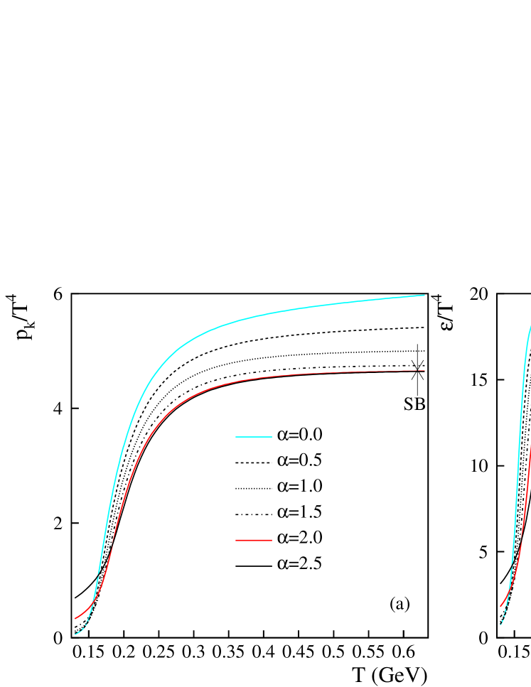
Figure 3: (Color online) Left panel (a): The ratio $p_{k}(\infty,T)/T^{4}$ calculated with the isobaric partition function for various values of $\alpha$. Above $T_{0}$, the curves at $\alpha=2.0$ and $\alpha=2.5$ are practically coincident. Right panel (b): The corresponding value of $\varepsilon/T^{4}$.

As one can see, the results depend on the choice of $\alpha$. For $\alpha=0$ and $1/2$, the curves grow with the temperature with larger slopes for smaller $\alpha$’s. Instead, for $1\leq\alpha\leq 5/2$, they settle onto constant asymptotic values (as we have verified numerically up to $T\sim 6$ GeV). As $\alpha$ change from $1$ to $5/2$ the asymptotic value converges very fast to $1/k^{4}=4.67$ (the Stefan-Boltzmann limit) from above. As shown in the plot, the curves practically coincide with the Stefan-Boltzmann limit already for $\alpha=2$. This behavior can be understood by inspecting the solution $s_{0}(T)=p_{k}(\infty,T)/T$ for the pressure. Because $s_{0}(T)$ is always larger than $s_{f}(T)$, we have

$$p_{k}(\infty,T)>\frac{T^{4}}{k^{4}}-B\;$$ (31)

and for $T\rightarrow\infty$

$$\frac{p_{k}(\infty,T)}{T^{4}}\gtrsim\frac{1}{k^{4}}\;.$$ (32)

The pressure $p_{k}(\infty,T)$ converges to $T^{4}/k^{4}$ only for sufficiently large values of $\alpha$, when the solutions $s_{0}(T)$ and $s_{f}(T)$ get closer and closer as $T\rightarrow\infty$.

In Fig. (3b), we plot the ratio $\varepsilon/T^{4}$, where $\varepsilon$ has been evaluated numerically by using the relation:

$$\varepsilon=T\frac{\partial p_{k}}{\partial T}-p_{k}\;.$$ (33)

Again this quantity converges to a finite asymptotic limit only for $1\leq\alpha\leq 5/2$ and, as before, coincides with the massless gas limit $3/k^{4}\sim 14$ for $\alpha=2$ and $\alpha=5/2$. The overall behavior is roughly the same as LQCD except for a small “horn” right above $T_{0}$. A closer look reveals that this is due to the constant bag pressure $B$ that produces a contribution $\sim B$ to the energy density of the system. Being a constant term its contribution to $\epsilon/T^{4}$ becomes negligible at high temperatures.

In Fig. (4a), the ratio $(\varepsilon-3p_{k})/T^{4}$ is plotted up to $T=0.6$ GeV. This quantity corresponds to the trace of the energy-momentum tensor $\Theta^{\mu\mu}(T)/T^{4}$, which is actually the fundamental quantity calculated in LQCD Cheng:2007jq . In Fig. (4b), we plot the ratio $s/T^{3}\equiv(\varepsilon+p_{k})/T^{4}$, where $s$ is the entropy density. Again, for $\alpha=0$ and $1/2$, the curves do not converge to a constant value, as expected from the previous results for $\varepsilon$ and $p_{k}$.

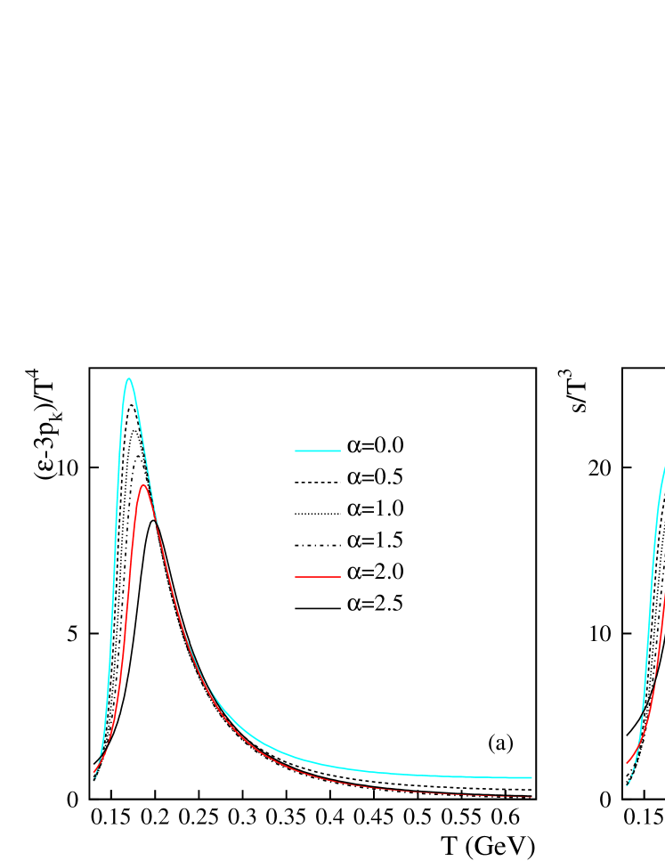
Figure 4: (Color online) Left panel (a): the ratio $(\varepsilon-3p_{k})/T^{4}$. Right panel (b): The ratio $s/T^{3}$, where $s$ is the entropy-density.

In our scheme, the pressure $p_{k}$ (and thus the energy density and the entropy) exceeds the corresponding Stefan-Boltzmann limit, except for $\alpha=2$ and $5/2$ where it converges to it. To obtain a lower pressure (at least at finite temperatures) one needs to further reduce the effective degrees of freedom of the system. This could be possibly achieved by introducing a surface energy term. In addition to the fact that part of the energy of the system would be spent to create the bags surface, such a contribution would favor spherically shaped bags, resulting in a further suppression of the accessible phase space. Probably, a similar effect could be also obtained including some residual repulsive interaction of the van der Waals type.

We stress that the general behavior of our model for the pressure, energy- and entropy-density cannot be obtained by simply introducing an upper mass-cutoff on the exponential spectrum in Eq. (II): the entropy-density would considerably exceed that obtained from LQCD even if we kept only masses up to $2$ GeV. In addition, the system would reach the massless gas limit only at temperatures much higher than the cutoff itself. On the other hand, in our model it is absolutely essential to assume an infinite mass spectrum. Otherwise the flat behavior in Fig. (3) and on Fig. (4b) would be spoiled and all these quantities would decrease with the temperature.

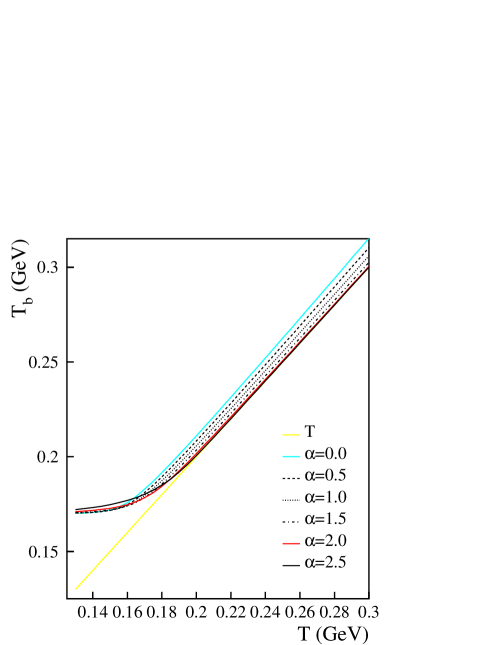
Figure 5: (Color online) The average effective bag temperature. The $45^{\circ}$’s straight line corresponds to the system temperature $T$.

It is also interesting to plot the average bag effective “temperature” $T_{b}\equiv k(p_{k}+B)^{1/4}$. As shown in Fig. (5), for $\alpha=2$ and $\alpha=5/2$ this converges to $T$ very quickly above $T_{0}$. For $\alpha=3/2$ or smaller the effective bag temperature is always larger than the system temperature. This fact is a direct consequence of the inequality in Eq. (31) that gives

$$T_{b}=k(p_{k}+B)^{1/4}>T\;,$$ (34)

Notice also that in the region $T<T_{0}$, $T_{b}\approxeq T_{0}$ for any value of $\alpha$. In other words, the pressure $p_{k}$ is negligible with respect to $B$ and the system behaves as a standard hadron gas. It is worth mentioning that in our framework the compressible hadrons can exchange energy only through a mechanical work (compression). They are, therefore, thermally insulated from the rest of the system and the bag temperature, as well as the entropy, must be understood as quantities that measure the degeneracy of the hadronic states.

Finally, for $1\leq\alpha\leq 5/2$, our model seems to produce a smooth crossover transition toward a new regime whose features are very similar to those of a gas of massless particles, even though no deconfined states are included in the partition function. To better understand this behavior it is useful to study the particles density $\langle n\rangle\equiv\langle N\rangle/V$ (Fig. (6a)) and the filling fraction ($f.f.$) (Fig. (6b)) which is defined as:

$$f.f.\equiv\frac{\langle V_{\rm hadrons}\rangle}{V}\;,$$ (35)

where $\langle V_{\rm hadrons}\rangle$ is the average volume occupied by the hadrons (for a rigorous definition and formula see Appendix B). The particles density can be calculated from the isobaric partition function by introducing a fictitious fugacity $\lambda$ (to be set to 1 afterward) for each particle in the system, i.e. replacing $Z(V,T)$ with

$$Z(V,T,\lambda)\equiv\sum_{N=0}^{\infty}\lambda^{N}Z_{N}(V,T)\;.$$ (36)

Accordingly, the isobaric partition function in Eq. (26) becomes

$$\widehat{Z}(T,s,\lambda)=\frac{1}{s-\lambda f(T,s)}$$ (37)

and the corresponding solution for the pressure $p_{k}\equiv p_{k}(\infty,T,\lambda)$. In the infinite volume limit, the particles density can be then obtained as:

$$\langle n\rangle=\lim_{V\rightarrow\infty}\frac{1}{V}\left.\frac{\partial\ln Z(V,T,\lambda)}{\partial\lambda}\right|_{\lambda=1}=\frac{1}{T}\left.\frac{\partial p_{k}(\infty,T,\lambda)}{\partial\lambda}\right|_{\lambda=1}$$ (38)

where in the last equality we have used the known relation $\ln Z=pV/T$.

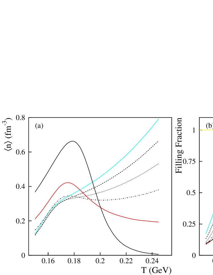
Figure 6: (Color online) Left panel (a): average number of particles per unit volume. Right panel (b): The filling fraction ($f.f.$). The horizontal line $f.f.=1$ has been drawn for reference.

As shown in Fig. (6a), the particles density grows very rapidly as $T$ approaches $T_{0}$ from below. This is qualitatively what one expects for the hadron gas, where the average number of particles shows a monotonically growing behavior. Conversely, for $T>T_{0}$ this quantity depends very strongly on the choice of the parameter $\alpha$. For $\alpha=0$, $1/2$ and $1$ we observe a change in the slope, but the curves still grow monotonically. For $\alpha=1.5$ and $2$ the particles density has a local minimum at $T\sim 0.2$ GeV and $T\sim 0.27$ GeV, respectively (the latter lies outside the plotted region), and then it starts growing again with smaller slopes for larger values of $\alpha$. For $\alpha=5/2$ the local minimum has disappeared, and after a sharp maximum at $T\sim 0.18$ GeV the particles density goes to zero. This is the effect of the finite size of hadrons, which tends to saturate the available system volume. In fact, as shown in Fig. (6b), when $T<T_{0}$ the filling fraction, Eq. (35), is relatively small, whereas for higher temperatures, the system is almost totally filled by extended particles, i.e. $\langle V_{\rm hadrons}\rangle\sim V$. In this scenario, the space and the phase space available is strongly suppressed, and the system tends to be populated by a smaller number of heavy particles. This effect is strongest for $\alpha=5/2$ (the filling fraction converges very fast to 1) and therefore $\langle n\rangle\rightarrow 0$. For smaller values of $\alpha$ this saturation effect becomes slightly less pronounced. A closer inspection reveals that for $\alpha<1$ the filling fraction has a maximum at very high temperature and then decreases with a very small slope, whereas for $\alpha=1$ it seems to settle to a constant value $f.f.\sim 0.98$. The phase space, therefore, is never entirely suppressed.

The behavior of the system changes continuously by varying $\alpha$. A numerical analysis indicates that there exist a value $\alpha_{0}$ between $2.12$ and $2.13$ such that, at high $T$, the particles density vanishes for any $\alpha_{0}<\alpha\leq 2.5$. In this range, the system is populated by one or few infinitely extended hadrons that occupy the entire space, filling the system with their inner QGP matter, which is a possible scenario for the deconfined phase. Conversely, for $1\leq\alpha\leq\alpha_{0}$, we find many, rather heavy,“squeezed” hadrons, which nonetheless mimic an ideal gas of massless particles. The number of particles, however, might be affected by the introduction of a surface energy term in the spectrum in Eq. (6). Such a term would result in an energy cost associated with the splitting of a large hadron into many smaller ones and might then widen the range of values for $\alpha$ that lead to $\langle n\rangle\simeq 0$ at temperatures above $T_{0}$.

Note that, even though $\langle n\rangle$ can have a minimum or even vanish, the entropy of the system always increases monotonically with the temperature (see Fig. (4b)). This is due to the fact that the dominant contribution (already at $T\sim T_{0}$) comes from the bags entropies. This has been checked by using the classical expression for a gas with $\langle N\rangle$ particles (with the excluded volume correction) and degeneracy $g$:

$$S\sim S_{\rm class}(\langle N\rangle,g)=S_{\rm class}(\langle N\rangle,g\equiv 1)+\langle N\rangle\ln g\;.$$

The contribution $\langle N\rangle\ln g$ corresponds to the sum of the bag entropies in Eq. (18), and it is dominant at high $T$.

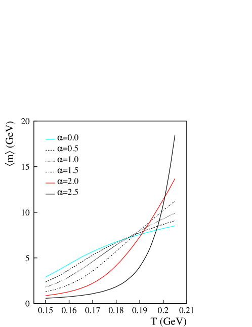
Figure 7: (Color online) Average hadrons mass.

Another interesting quantity is the average hadron mass $\langle m\rangle$, shown in Fig. (7) that has been evaluated according to

$$\langle m\rangle=\frac{\varepsilon}{\langle n\rangle}-\frac{3}{2}T\;$$ (39)

As one can see, smaller values of $\alpha$ correspond to higher $\langle m\rangle$ at low temperature, whereas the situation is reversed at high $T$. This follows from Eq. (39) as a direct consequence of the behavior of $\langle n\rangle$ (Fig. (6a)). For $\alpha=5/2$ the average mass $\langle m\rangle$ grows with the temperature with the maximum slope and diverges when $\langle n\rangle\rightarrow 0$, i.e. when the system is populated by a finite number of infinite “hadrons”.

In the vicinity of the transition region $\langle m\rangle$ varies from $4.34$ GeV (for $\alpha=0$) to $0.75$ GeV (for $\alpha=5/2$) at $T=0.16$ GeV, and from $5.70$ GeV to $1.08$ at $T=0.17$ GeV, for $\alpha=0$ and $5/2$, respectively. These values will somewhat depend on the choice of the model parameters. They would depend even more on an eventual upper mass cutoff. In fact, the high value of $\langle m\rangle$ for $\alpha=0$ results from our assumption of an infinite mass spectrum and already at $T=0.16$ GeV it falls outside the region of the known hadrons. Our estimates are, however, lower than what one obtains for an exponential spectrum of point-like hadrons as in Eq. (II). In such a case, for $\alpha=0$ the average mass is $\langle m\rangle=6.80$ GeV at $T=0.16$ GeV and infinity at $T=T_{0}=0.17$ GeV (the partition function itself is divergent). A mass cutoff at $2.0$ GeV would reduce these numbers to $\langle m\rangle=1.36$ GeV and $\langle m\rangle=1.43$ GeV at $T=0.16$ GeV and $T=0.17$ GeV, respectively.

III.1 Consistency check

As a final remark, we want to discuss the consistency of the model. To check this point we must make sure that quantities such as the energy density (that we have evaluated from the pressure by using Eq. (33)) correspond to a thermal average of the form

$$\varepsilon=\frac{1}{V}\frac{\sum_{\rm states}E_{\rm state}\textrm{e}^{-E_{\rm state}/T}}{\sum_{\rm states}\textrm{e}^{-E_{\rm state}/T}}\;.$$ (40)

A first hint in this direction, is given, a posteriori, by the results shown in this section, particularly, by quantities such as the filling fraction. The $f.f.$ has been evaluated by making use of the relation in Eq. (39) (see Appendix B) that implicitly relies on a form like Eq. (40) for the energy density. Indeed, a wrong thermodynamical interpretation of $\varepsilon$ would likely have lead to dramatic consequences on the filling fraction, which contrarily assumes only physical values in the interval $[0,1]$. However, to make a more direct test, we will provide an approximate expression for the grand-canonical partition function and we will compare $\varepsilon$ in Fig. (3b) with its corresponding value obtained as in Eq. (40). This can be done for the case $\alpha=3/2$. For this particular value of $\alpha$ the multiple integrals over $\{{\rm d}\eta_{i}\}$ in Eq. (23) can be reduced to an unidimensional integral (see Appendix C) that greatly facilitates the numerical treatment. Although, as demonstrated in this section, results do depend on the choice of $\alpha$, for the range of $0\leq\alpha\leq 5/2$, one can hope that the following arguments will be still valid.

Using $\alpha=3/2$ in Eq. (23) we get for the partition function

$$Z(V,T)=\sum_{N=0}^{\infty}Z_{N}(V,T)$$ (41)

with

$$Z_{N}(V,T)=\left[c_{0}\left(\frac{T}{2\pi}\right)^{3/2}\right]^{N}\frac{1}{N!}\left[\prod_{i=1}^{N}\int_{m_{c}}^{\infty}{\rm d}\eta_{i}\right]$$

$$\times\exp{\left\{\left[\frac{1}{kp_{r,N}^{1/4}}-\frac{1}{T}\left(\frac{3}{4}+\frac{B}{4p_{r,N}}\right)\right]\sum_{i=1}^{N}\eta_{i}\right\}}$$ (42)

$$\times\left(V-\sum_{i=1}^{N}\frac{\eta_{i}}{4p_{r,N}}\right)^{N}\Theta{\left(V-\sum_{i=1}^{N}\frac{\eta_{i}}{4p_{r,N}}\right)}\;.$$

Here we have added the suffix $N$ to $p_{r}$ to indicate the dependence of the pressure $p_{r,N}$ on the particle number in the canonical ensemble. The pressure $p_{r,N}$ is now just a parameter of the model. To determine its value, we need to find the value of $p_{r,N}$ that maximizes the logarithm of the integrand in Eq. (III.1):

$$\Phi=\left[\frac{1}{kp_{r,N}^{1/4}}-\frac{1}{T}\left(\frac{3}{4}+\frac{B}{4p_{r,N}}\right)\right]\sum_{i=1}^{N}\eta_{i}+N\log\left(V-\sum_{i=1}^{N}\frac{\eta_{i}}{4p_{r,N}}\right)\;,$$ (43)

where (for the moment) we omit the $\Theta$ function. The above expression depends on $\mathscr{M}\equiv\sum_{i=1}^{N}\eta_{i}$. To simplify the following derivation, we will introduce an approximation. Instead of solving $\partial\Phi/\partial p_{r,N}=0$ for a generic set $\eta_{1},\ldots,\eta_{N}$, we find a solution for the most important configurations defined by the value $\tilde{\mathscr{M}}$ that maximizes the integrand. In other words, we solve the system of equations:

$$\left\{\begin{array}[]{rl}&\frac{\partial\Phi}{\partial\mathscr{M}}=0\\ &\frac{\partial\Phi}{\partial p_{r,N}}=0\end{array}\right.\;.$$ (44)

Note that the second condition ensures that $\varepsilon=T^{2}(\partial\ln Z/\partial T)/V$ has the form of Eq. (40) as any implicit dependence on $T$ of $p_{r,N}$ do not contribute to $\partial\ln Z/\partial T$. In fact, if we denote with $\partial^{*}\ln Z/\partial T$ the derivative performed only on the explicit $T$ dependence of $\ln Z$ we have

$$\frac{\partial\ln Z}{\partial T}=\frac{\partial^{*}\ln Z}{\partial T}+\frac{1}{Z}\sum_{N=0}^{\infty}\frac{\partial Z_{N}}{\partial p_{r,N}}\frac{\partial p_{r,N}}{\partial T}$$ (45)

where the second term vanishes because of the second condition in Eq. (44). The Eq. (44) results in (see Appendix D):

$$\tilde{p}_{r,N}=B+\frac{NT}{\left(V-\frac{\tilde{\mathscr{M}}}{4\tilde{p}_{r,N}}\right)}\;.$$ (46)

The interpretation of the above expression is straightforward. Writing $\tilde{p}_{r,N}\equiv B+\tilde{p}_{k,N}$ one obtains the equivalent equation:

$$\tilde{p}_{k,N}\equiv\frac{NT}{V-\frac{\tilde{\mathscr{M}}}{4(B+\tilde{p}_{k,N})}}\;.$$ (47)

Here, the right-hand side of Eq. (47) is simply the canonical pressure of an ideal gas of $N$ particles with the total volume $V$ replaced by the available volume $(V-\sum_{i}^{N}V_{i})$. It is then natural to identify $p_{k,N}$ with the kinetic pressure in the canonical ensemble. Of course, once averaged over $N$ and over $\{\eta_{i}\}$, for a sufficiently large $V$, this pressure must coincide with $p_{k}(\infty,T)$ evaluated with the isobaric partition function. Eq. (47) has the form of a self-consistency relation, as $\tilde{p}_{k,N}$ appears also in the right-hand side in the excluded volume term. Eq. (47) is a quadratic form and has two solutions: a negative and positive one, and the negative corresponds to the situation where volume of hadrons exceeds the total volume, $\sum_{i=1}^{N}V_{i}>V$. The positive solution on the other hand ensures $\sum_{i=1}^{N}V_{i}\leq V$ and therefore the condition for the $\Theta$ function in Eq. (III.1) is always fulfilled. In what follows, we will adopt the positive solution of the Eq. (47) for any $\{\eta_{1},\ldots,\eta_{N}\}$ (not only for the most probable set $\sum_{i}^{N}\eta_{i}=\tilde{\mathscr{M}}$) and we will integrate numerically $Z_{N}(V,T)$ in the variables $\{\eta_{i}\}$. The partition function $Z(V,T)$ is then evaluated by summing over the particle number $N$ up to a cutoff $N_{cut}$

$$Z(V,T)=\sum_{N=0}^{N_{cut}}Z_{N}(V,T)$$ (48)

where $N_{cut}$ is sufficiently large to ensure the accuracy of our calculations. Finally we test the consistency of our picture by comparing the ratios $p_{k}/T^{4}$ and $\varepsilon/T^{4}$ with the results obtained with the isobaric partition function.

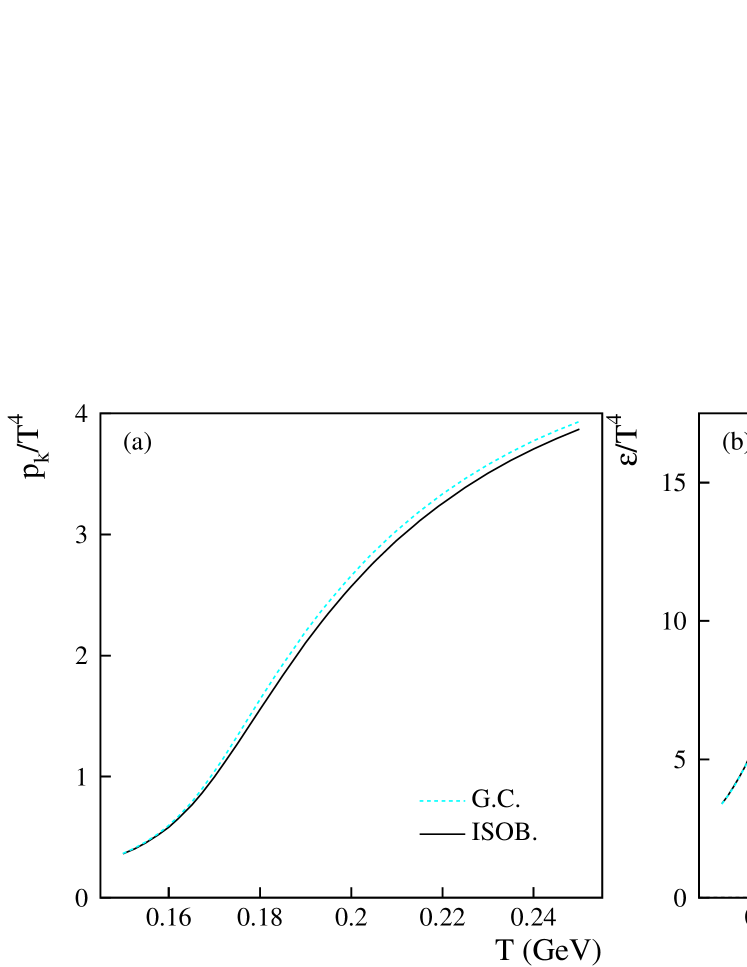
Figure 8: (Color online) Left panel (a): Comparison between the ratio $p_{k}/T^{4}$ evaluated with the isobaric partition function (solid line) and with the grand canonical partition function (dashed line). Right panel (b): The same as in the left panel for the corresponding ratio $\varepsilon/T^{4}$.

In Fig. (8), the ratios $p_{k}/T^{4}$ (left panel) and $\varepsilon/T^{4}$ (right) have been evaluated with the isobaric partition function (solid line) and with the grand canonical partition function (dashed line) for a volume $V=6.4\cdot 10^{4}$ GeV^-3, which is, as we checked, a good approximation of the infinite volume limit. As one can see, in both cases the two curves are very close, actually for the energy density they are practically coincident. The small (expected) difference between the isobaric and the grand-canonical result reflects the quality of our approximation. The same test has been also performed on the entropy density, the particles density and the filling fraction. For all these quantities we have observed an equally good agreement.

IV Conclusions and Discussion

In this article, we have studied the crossover transition of the gas of bags Gorenstein:1998am . We have found that the behavior of the system depends sensitively on the parameter $\alpha$ of the Hagedorn-like mass spectrum $\rho(m)=c_{0}m^{-\alpha}\exp{\{m/T_{0}\}}$. The system exhibits a crossover transition for $0\leq\alpha\leq 5/2$ and an actual phase transition for larger values. In the range $0\leq\alpha\leq 5/2$ we made a coarse scan of $\alpha$, setting $\alpha=0$, $1/2$, $1$, $3/2$, $2$ and $5/2$. For $1\leq\alpha\leq 5/2$ the gas of bags undergoes a sharp (yet, continuous) transition qualitatively similar to lattice QCD. In this range, the asymptotic values of $p/T^{4}$, $\varepsilon/T^{4}$, $s/T^{3}$, coincide with the Stefan Boltzmann limit for $\alpha=2$ and $\alpha=5/2$, whereas they settle to slightly larger values for $\alpha=3/2$ and $1$. For $\alpha=0$ and $1/2$, these quantities grow indefinitely with the temperature with small, decreasing, slopes going from $\alpha=0$ to $\alpha=1/2$. We have also studied the (strong) dependence of the particles density $\langle n\rangle=\langle N\rangle/V$ (where $V\rightarrow\infty$) on $\alpha$. We have found that there exist a limiting value $\alpha_{0}$ between $2.12$ and $2.13$ such that for $\alpha_{0}<\alpha\leq 5/2$ the particles density vanishes at high temperature. The system is then populated by one (or few) infinite bag(s) that occupies the entire volume. Conversely, for $\alpha<\alpha_{0}$, $\langle n\rangle$ grows with the temperature. In the range $1\leq\alpha<\alpha_{0}$, the ideal gas behavior is mimicked by a number of heavy extended bags that saturates the phase space forming a dense system. A pictorial representation summarizing the various high-temperature phases of the model is given in Fig. (9).

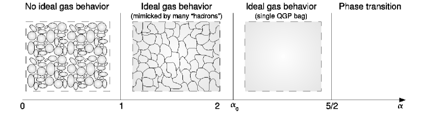
Figure 9: Pictorial representation of the various high-temperature phases of the model as a function of $\alpha$. The scale has been distorted for visual reasons.

In this work we have explored a simple, intuitive model for a gas of hadrons in the vicinity of the transition at vanishing baryochemical potential. To this end, we have adopted the idea of the MIT bag model and we have described hadrons as extended QGP bags. We have shown that, in the vicinity of $T_{0}$ (which is directly related to the transition temperature of our model), elastic interactions among hadrons play a fundamental role. In our schematic approach, they are quantified by the thermal pressure $p_{k}$. The effect of $p_{k}$ is to squeeze the hadrons, and for a certain set of model parameters, $1\leq\alpha\leq 5/2$, the ideal gas behavior at high temperature can be reproduced. At the same time, the effective inner “temperature”, or rather degeneracy parameter, $T_{b}$, of the bags increases with $p_{k}$, resulting in a temperature-dependent mass spectrum. Above $T_{0}$, the physical picture of the QGP phase corresponds to a number $\sim 1$ of infinite bags that occupy the entire space. This is indeed the situation for $\alpha_{0}<\alpha\leq 5/2$. On the other hand, a large number of independent QGP bags (such as for $\alpha<\alpha_{0}$) would contradict the lattice findings of vanishing flavor-flavor correlations Koch:2005vg ; Allton:2005gk ; Gavai:2005yk . However, in order to define precisely the range of values of $\alpha$ that lead to a consistent QGP scenario, it is fundamental to study the effect of a surface energy term. This contribution disfavors configurations with a large number of particles (they are more “expensive” in terms of surface energy) and might reduce the number of bags in the high-temperature phase, widening the range of possible values for $\alpha$.

Future work will likely concentrate on the effect of surface energy terms in addition to the study of van der Waals type residual interactions. It would be also interesting to analyze in detail the behavior of the system at finite baryochemical potential. This could be done starting from the formalism developed in Gorenstein:2005rc .

V Acknowledgments:

The authors thank M. I. Gorenstein for a critical reading of the manuscript and for useful suggestions. This work is supported by the Director, Office of Energy Research, Office of High Energy and Nuclear Physics, Divisions of Nuclear Physics, of the U.S. Department of Energy under Contract No. DE-AC02-05CH11231.

Appendix A

By using the equations (16) and (25), the isobaric partition function in Eq. (24) can be conveniently written as:

$$\widehat{Z}(T,s)=\sum_{N=0}^{\infty}\frac{1}{N!}\left[\prod_{i=1}^{N}\int_{m_{c}}^{\infty}{\rm d}\eta_{i}\right]h_{N}(\{\eta_{i}\},T,s)$$ (49)

$$\times\int_{0}^{\infty}{\rm d}V\exp{\left[-sV\right]}\left(V-\sum_{i=1}^{N}\frac{\eta_{i}}{4(B+sT)}\right)^{N}\Theta{\left(V-\sum_{i=1}^{N}\frac{\eta_{i}}{4(B+sT)}\right)}$$

where

$$h_{N}(\{\eta_{i}\},T,s)\equiv\left(\frac{T}{2\pi}\right)^{3N/2}c_{0}^{N}\left[\prod_{i=1}^{N}\left(\frac{3}{4}\eta_{i}+B\frac{\eta_{i}}{4(B+sT)}\right)^{3/2-\alpha}\right]$$

$$\times\exp{\left\{\left[\frac{1}{k(B+sT)^{1/4}}-\frac{1}{T}\left(\frac{3}{4}+\frac{B}{4(B+sT)}\right)\right]\sum_{i=1}^{N}\eta_{i}\right\}}\;.$$ (50)

The integral over ${\rm d}V$ can be carried out

$$\int_{0}^{\infty}{\rm d}V\exp{\left[-sV\right]}\left(V-\sum_{i=1}^{N}\frac{\eta_{i}}{4(B+sT)}\right)^{N}\Theta{\left(V-\sum_{i=1}^{N}\frac{\eta_{i}}{4(B+sT)}\right)}$$ (51)

$$=\frac{N!}{s^{N+1}}\exp{\left\{-\sum_{i=1}^{N}\eta_{i}\frac{s}{4(B+sT)}\right\}}\;.$$

and Eq. (49) becomes:

$$\widehat{Z}(T,s)=\frac{1}{s}\sum_{N=0}^{\infty}\left[\prod_{i=1}^{N}\int_{m_{c}}^{\infty}{\rm d}\eta_{i}\right]\frac{h_{N}(\{\eta_{i}\},T,s)}{s^{N}}\exp{\left\{-\sum_{i=1}^{N}\eta_{i}\frac{s}{4(B+sT)}\right\}}\;.$$ (52)

The multiple integral in the last equation, can be factorized as:

$$\left[\prod_{i=1}^{N}\int_{m_{c}}^{\infty}{\rm d}\eta_{i}\right]h_{N}(\{\eta_{i}\},T,s)\exp{\left\{-\sum_{i=1}^{N}\eta_{i}\frac{s}{4(B+sT)}\right\}}\equiv f(T,s)^{N}\;.$$ (53)

One then obtains Eq. (26) with $f(T,s)$ given by Eq. (27).

Appendix B

By using Eq. (17), we write the average volume occupied by hadrons as

$$\langle V_{\rm hadrons}\rangle=\langle N\rangle\frac{\langle U\rangle}{3p_{r}}=\langle N\rangle\frac{\langle m\rangle}{3p_{r}+B}=\langle N\rangle\frac{\langle m\rangle}{3p_{k}+4B}\;,$$ (54)

where we used the stability condition $p_{r}=p_{k}+B$. In turn, the average mass $\langle m\rangle$ reads (see also Eq. (39)):

$$\langle m\rangle=\frac{\varepsilon}{\langle n\rangle}-\frac{3}{2}T\;.$$ (55)

The filling fraction $f.f.$ can then be expressed in terms of $\varepsilon$, $p_{k}$ and the particles density $\langle n\rangle$ as:

$$f.f\equiv\frac{\langle V_{\rm hadrons}\rangle}{V}=\frac{\varepsilon-3/2\langle n\rangle T}{3p_{k}+4B}\;.$$ (56)

Appendix C

The partition function of $N$ particles can be reduced to a unidimensional integral when $\alpha=3/2$ as the factor $\left(3/4\eta_{i}+BV_{i}\right)^{3/2-\alpha}$ reduces to 1. Let us begin by making the substitution: $\eta_{i}\rightarrow y^{2}_{i}+m_{c}$ that gives for $Z_{N}$ in Eq. (III.1):

$$Z_{N}=\left[2c_{0}\left(\frac{T}{2\pi}\right)^{3/2}\right]^{N}\frac{1}{N!}\left[\prod_{i=1}^{N}\int_{0}^{\infty}{\rm d}y_{i}\;y_{i}\right]\left(V-\frac{Nm_{c}}{4p_{r,N}}-\sum_{i=1}^{N}\frac{y^{2}_{i}}{4p_{r,N}}\right)^{N}$$

$$\times\exp{\left\{\left[\frac{1}{kp_{r,N}^{1/4}}-\frac{1}{T}\left(\frac{3}{4}+\frac{B}{4p_{r,N}}\right)\right]\left(\sum_{i=1}^{N}y^{2}_{i}+Nm_{c}\right)\right\}}\;.$$ (57)

It is now convenient to rewrite our integral by using $N$-dimensional hyperspherical coordinates by setting:

$$y_{1} = r\cos{\phi_{1}}$$ (58)

$$y_{2} = r\sin{\phi_{1}}\cos{\phi_{2}}$$

$$y_{3} = r\sin{\phi_{1}}\sin{\phi_{2}}\cos{\phi_{3}}$$

$$\vdots$$

$$y_{N} = r\sin{\phi_{1}}\sin{\phi_{2}}\ldots\sin{\phi_{N-1}}\;,$$

and

$${\rm d}^{N}r=r^{N-1}\sin^{N-2}{\phi_{1}}\sin^{N-3}{\phi_{2}}\ldots\sin{\phi_{N-2}}\;{\rm d}r\;{\rm d}\phi_{1}\ldots{\rm d}\phi_{N-1}\;.$$ (59)

with

$$r^{2}\equiv\sum_{i}^{N}y^{2}_{i}\;.$$ (60)

We now note that, apart from ${\rm d}y_{i}\;y_{i}$, the integrand in Eq. (57) depends only on $r^{2}$. This is true also for the pressure $p_{r,N}=B+p_{k,N}$, where $p_{k,N}$ is given by the equations (47) and, in the new variables, reads:

$$p_{k,N}=\frac{1}{6V}\left(\xi+\sqrt{36B\,T\,N\,V+\xi^{2}}\right)$$ (61)

where

$$\xi=3TN+\frac{3}{4}\left(r^{2}+Nm_{c}\right)-3BV\;.$$ (62)

Eq. (57) can now be written as:

$$Z_{N}=\left[2c_{0}\left(\frac{T}{2\pi}\right)^{3/2}\right]^{N}$$

$$\times\frac{1}{N!}\int_{0}^{\infty}{\rm d}r\;r^{N-1}\int_{0}^{\frac{\pi}{2}}{\rm d}\phi_{1}\ldots\int_{0}^{\frac{\pi}{2}}{\rm d}\phi_{N-1}\sin^{N-2}{\phi_{1}}\sin^{N-3}{\phi_{2}}\ldots\sin{\phi_{N-2}}$$

$$\times r^{N}\left[\prod_{i=1}^{N-1}\cos{\phi_{i}}\right]\sin^{N-1}{\phi_{1}}\sin^{N-2}{\phi_{2}}\ldots\sin{\phi_{N-1}}\left(V-\frac{Nm_{c}}{4p_{r,N}}-\frac{r^{2}}{4p_{r,N}}\right)^{N}$$

$$\times\exp{\left\{\left[\frac{1}{kp_{r,N}^{1/4}}-\frac{1}{T}\left(\frac{3}{4}+\frac{B}{4p_{r,N}}\right)\right]\left(r^{2}+Nm_{c}\right)\right\}}\;.$$ (63)

Next we separate Eq. (Appendix C) into an angular integral, $A_{N}$, and a radial integral, $I_{N}$, such that:

$$Z_{N}=\left[2c_{0}\left(\frac{T}{2\pi}\right)^{3/2}\right]^{N}\frac{1}{N!}A_{N}I_{N}$$ (64)

where:

$$A_{N}=\int_{0}^{\frac{\pi}{2}}{\rm d}\phi_{1}\ldots\int_{0}^{\frac{\pi}{2}}{\rm d}\phi_{N-1}\sin^{N-2}{\phi_{1}}\sin^{N-3}{\phi_{2}}\ldots\sin{\phi_{N-2}}$$ (65)

$$\times\left[\prod_{i=1}^{N-1}\cos{\phi_{i}}\right]\sin^{N-1}{\phi_{1}}\sin^{N-2}{\phi_{2}}\ldots\sin{\phi_{N-1}}\;,$$

and

$$I_{N}=\int_{0}^{\infty}{\rm d}r\;r^{2N-1}\left(V-\frac{Nm_{c}}{4p_{r,N}}-\frac{r^{2}}{4p_{r,N}}\right)^{N}$$ (66)

$$\times\exp{\left\{\left[\frac{1}{kp_{r,N}^{1/4}}-\frac{1}{T}\left(\frac{3}{4}+\frac{B}{4p_{r,N}}\right)\right]\left(r^{2}+Nm_{c}\right)\right\}}\;.$$

The angular integral $A_{N}$ can be solved by applying the following recursion relation:

$$A_{N}=A_{N-1}\int_{0}^{\frac{\pi}{2}}{\rm d}\phi\sin^{2N-3}{\phi}\;\cos{\phi}=\frac{A_{N-1}}{2(N-1)}\;.$$ (67)

yielding

$$A_{N}=\frac{A_{N-1}}{2(N-1)}=\frac{A_{N-2}}{2^{2}(N-1)(N-2)}=\frac{A_{N-3}}{2^{3}(N-1)(N-2)(N-3)}\;.\ldots$$ (68)

Accordingly, by using $A_{2}=1/2$ one obtains:

$$A_{N}=\frac{1}{2^{N-1}(N-1)!}\;.$$ (69)

The Eq. (Appendix C) then reduces to:

$$Z_{N}=\left[2c_{0}\left(\frac{T}{2\pi}\right)^{3/2}\right]^{N}\frac{1}{N!}\frac{1}{2^{N-1}(N-1)!}\int_{0}^{\infty}{\rm d}r\;r^{2N-1}$$ (70)

$$\times\left(V-\frac{Nm_{c}}{4p_{r,N}}-\frac{r^{2}}{4p_{r,N}}\right)^{N}\exp{\left\{\left[\frac{1}{kp_{r,N}^{1/4}}-\frac{1}{T}\left(\frac{3}{4}+\frac{B}{4p_{r,N}}\right)\right]\left(r^{2}+Nm_{c}\right)\right\}}\;.$$

Appendix D

Performing the derivatives, the system in Eq. (44) reads

$$\left\{\begin{array}[]{rl}&\frac{1}{kp_{r,N}^{1/4}}=\frac{N}{4p_{r,N}}\frac{1}{\left(V-\frac{\mathscr{M}}{4p_{r,N}}\right)}+\frac{1}{T}\left(\frac{3}{4}+\frac{B}{4p_{r,N}}\right)\\ &\frac{1}{kp_{r,N}^{1/4}}=\frac{B}{Tp_{r,N}}+\frac{N}{p_{r,N}}\frac{1}{\left(V-\frac{\mathscr{M}}{4p_{r,N}}\right)}\end{array}\right.\;.$$ (71)

By subtracting the first equation from the second equation, one easily obtains Eq. (46).

References

- (1) R. Hagedorn, in Erice 1972, Proceedings of the Study Institute On High Energy Astrophysics (Cambridge University Press, Cambridge, 1974), pp. 255-296.
- (2) M. Creutz, L. Jacobs and C. Rebbi, Phys. Rev. D 20, 1915 (1979).
- (3) P. Braun-Munzinger, J. Stachel, J. P. Wessels and N. Xu, Phys. Lett. B 365, 1 (1996).
- (4) J. Cleymans, D. Elliott, H. Satz and R. L. Thews, Z. Phys. C 74, 319 (1997).
- (5) W. Broniowski, A. Baran and W. Florkowski, Acta Phys. Polon. B 33, 4235 (2002).
- (6) F. Becattini, J. Manninen and M. Gazdzicki, Phys. Rev. C 73, 044905 (2006).
- (7) A. Andronic, P. Braun-Munzinger, K. Redlich and J. Stachel, J. Phys. G 35, 104155 (2008).
- (8) J. Manninen and F. Becattini, Phys. Rev. C 78, 054901 (2008).
- (9) F. Becattini, Z. Phys. C 69, 485 (1996).
- (10) F. Becattini, in Proceedings of XXXIII Eloisatron Workshop on Universality Features in Multihadron Production and the leading effect edited by A. Zichichi (1996), pp. 74-104, hep-ph/9701275
- (11) F. Becattini and U. W. Heinz, Z. Phys. C 76, 269 (1997).
- (12) F. Becattini and G. Passaleva, Eur. Phys. J. C 23, 551 (2002).
- (13) F. Karsch, K. Redlich and A. Tawfik, Eur. Phys. J. C 29, 549 (2003).
- (14) M. Cheng et al., Phys. Rev. D 77, 014511 (2008).
- (15) D. H. Rischke, H. Stoecker, W. Greiner and B. L. Friman, J. Phys. G 14, 191 (1988).
- (16) M. Xu, M. Yu and L. Liu, Phys. Rev. Lett. 100, 092301 (2008).
- (17) R. Hagedorn and J. Rafelski, From Hadron Gas To Quark Matter. 1 CERN TH 2947 (1980).
- (18) J. Rafelski and R. Hagedorn, From Hadron Gas To Quark Matter. 2 CERN TH 2969 (1980).
- (19) J. I. Kapusta, Phys. Rev. D 23, 2444 (1981).
- (20) M. I. Gorenstein, V. K. Petrov and G. M. Zinovev, Phys. Lett. B 106, 327 (1981).
- (21) S. Kagiyama, A. Minaka and A. Nakamura, Prog. Theor. Phys. 89, 1227 (1993).
- (22) M. I. Gorenstein, W. Greiner and S. N. Yang, J. Phys. G 24, 725 (1998).
- (23) S. Kagiyama, S. Kumamoto, A. Minaka, A. Nakamura, K. Ohkura and S. Yamaguchi, Eur. Phys. J. C 25, 453 (2002), and references therein.
- (24) M. I. Gorenstein, M. Gazdzicki and W. Greiner, Phys. Rev. C 72, 024909 (2005).
- (25) I. Zakout, C. Greiner and J. Schaffner-Bielich, Nucl. Phys. A 781, 150 (2007).
- (26) K. A. Bugaev, Phys. Rev. C 76, 014903 (2007).
- (27) I. Zakout and C. Greiner, Phys. Rev. C 78, 034916 (2008).
- (28) Y. Aoki, G. Endrodi, Z. Fodor, S. D. Katz and K. K. Szabo, Nature 443, 675 (2006).
- (29) A. Chodos, R. L. Jaffe, K. Johnson, C. B. Thorn and V. F. Weisskopf, Phys. Rev. D 9, 3471 (1974).
- (30) F. Becattini and L. Ferroni, Eur. Phys. J. C 35, 243 (2004).
- (31) D. Stauffer, A. Aharony, Introduction to Percolation Theory, Taylor & Francis, London 1994.
- (32) A. Coniglio and W. Klein, J. Phys. A 13, 2775 (1980).
- (33) S. Fortunato and H. Satz, Phys. Lett. B 475, 311 (2000).
- (34) S. Fortunato and H. Satz, Nucl. Phys. A 681, 466 (2001).
- (35) S. Fortunato, F. Karsch, P. Petreczky and H. Satz, Nucl. Phys. Proc. Suppl. 94, 398 (2001).
- (36) S. Fortunato, F. Karsch, P. Petreczky and H. Satz, Phys. Lett. B 502, 321 (2001).
- (37) V. Koch, A. Majumder, and J. Randrup Phys. Rev. Lett. 95 182301 (2005).
- (38) C. R. Allton et al. Phys. Rev. D71 054508 (2005).
- (39) R. V. Gavai and S. Gupta Phys. Rev. D73 014004 (2006).