$\sqrt{\hat{s}}_{min}$: a global inclusive variable for determining the mass scale of new physics in events with missing energy at hadron colliders

Abstract:

We propose a new global and fully inclusive variable $\hat{s}^{1/2}_{min}$ for determining the mass scale of new particles in events with missing energy at hadron colliders. We define $\hat{s}^{1/2}_{min}$ as the minimum center-of-mass parton level energy consistent with the measured values of the total calorimeter energy E and the total visible momentum $\vec{P}$. We prove that for an arbitrary event, $\hat{s}^{1/2}_{min}$ is simply given by the formula $\hat{s}^{1/2}_{min}=\sqrt{E^{2}-P_{z}^{2}}+\sqrt{\not\!\!E_{T}^{2}+M_{inv}^{2}}$, where $M_{inv}$ is the total mass of all invisible particles produced in the event. We use $t\bar{t}$ production and several supersymmetry examples to argue that the peak in the $\hat{s}^{1/2}_{min}$ distribution is correlated with the mass threshold of the parent particles originally produced in the event. This conjecture allows an estimate of the heavy superpartner mass scale (as a function of the LSP mass) in a completely general and model-independent way, and without the need for any exclusive event reconstruction. In our SUSY examples of several multijet plus missing energy signals, the accuracy of the mass measurement based on $\hat{s}^{1/2}_{min}$ is typically at the percent level, and never worse than $10\%$. After including the effects of initial state radiation and multiple parton interactions, the precision gets worse, but for heavy SUSY mass spectra remains $\sim 10\%$.

1 Introduction

The ongoing Run II of the Fermilab Tevatron and the imminent run of the Large Hadron Collider (LHC) at CERN are on the hunt for new physics beyond the Standard Model (BSM) at the TeV scale. Arguably the most compelling phenomenological evidence for BSM particles and interactions at the TeV scale is provided by the dark matter problem [1], whose solution requires new particles and interactions BSM. A typical particle dark matter candidate does not interact in the detector and can only manifest itself as missing energy. At hadron colliders, where the total center of mass energy in each event is unknown, the missing energy is inferred from the imbalance of the total transverse momentum of the detected visible particles, and is commonly referred to as “missing transverse energy” (MET). The dark matter problem therefore greatly motivates the study of MET signatures at the Tevatron and the LHC [2].

While the MET class of BSM signatures is probably the best motivated one from a theoretical point of view, it is also among the most challenging from an experimental point of view. On the one hand, to get a good MET measurement, one needs to have all detector components working properly, since the mismeasurement of any one single type of objects would introduce fake MET. In addition, there are complications from cosmics, pile-up, beam halo, noise, etc. Therefore, establishing a MET signal due to some new physics is a highly non-trivial task [2, 3].

At the same time, interpreting a missing energy signal of new physics is quite challenging as well. The main stumbling block is the fact that we are missing some of the kinematical information from each event, namely the energies and momenta of the missing invisible particles. What is worse, a priori we cannot be certain about the exact number of missing particles in the event, or their identity, e.g. are they SM neutrinos, new BSM dark matter particles, or some combination of both? These difficulties are illustrated in Fig. 1, where we show the generic topology of the missing energy events that we are considering in this paper.

1.5 1.0   

Figure 1: The generic event topology under consideration in this paper. Black (red) lines correspond to SM (BSM) particles. The solid lines denote SM particles $X_{i}$, $i=1,2,\ldots,n_{vis}$, which are visible in the detector, e.g. jets, electrons, muons and photons. The SM particles may originate either from initial state radiation (ISR), or from the hard scattering and subsequent cascade decays (indicated with the green-shaded ellipse). The dashed lines denote neutral stable particles $\chi_{i}$, $i=1,2,\ldots,n_{inv}$, which are invisible in the detector. In general, the set of invisible particles consists of some number $n_{\chi}$ of BSM particles (indicated with the red dashed lines), as well as some number $n_{\nu}=n_{inv}-n_{\chi}$ of SM neutrinos (denoted with the black dashed lines). The identities and the masses $m_{i}$ of the BSM invisible particles $\chi_{i}$, ($i=1,2,\ldots,n_{\chi}$) do not necessarily have to be all the same, i.e. we allow for the simultaneous production of several different species of dark matter particles. The global event variables describing the visible particles are: the total energy $E$, the transverse components $P_{x}$ and $P_{y}$ and the longitudinal component $P_{z}$ of the total visible momentum $\vec{P}$. The only experimentally available information regarding the invisible particles is the missing transverse momentum $\not\!\!\vec{P}_{T}$.

As can be seen from the figure, we are imagining a completely general setup – each event will contain a certain number $n_{vis}$ of Standard Model (SM) particles $X_{i}$, $i=1,2,\ldots,n_{vis}$, which are visible in the detector, i.e. their energies and momenta are in principle measured. Examples of such visible SM particles are the basic reconstructed objects, e.g. jets, photons, electrons and muons. The visible particles $X_{i}$ are denoted in Fig. 1 with solid black lines and may originate either from initial state radiation (ISR), or from the hard scattering and subsequent cascade decays (indicated with the green-shaded ellipse). On the other hand, the missing energy $\not\!\!E_{T}$ (or more appropriately, the missing transverse momentum $\not\!\!\vec{P}_{T}$) will arise from a certain number $n_{inv}$ of stable neutral particles $\chi_{i}$, $i=1,2,\ldots,n_{inv}$, which are invisible in the detector. In general, the set of invisible particles in any event will consist of a certain number $n_{\chi}$ of BSM particles (indicated with the red dashed lines), as well as a certain number $n_{\nu}=n_{inv}-n_{\chi}$ of SM neutrinos (denoted with the black dashed lines). The missing energy measurement alone does not tell us the number $n_{inv}$ of missing particles, nor how many of them are neutrinos and how many are BSM (dark matter) particles. Notice that in this general setup the identities and the masses $m_{i}$ of the BSM invisible particles $\chi_{i}$, ($i=1,2,\ldots,n_{\chi}$) do not necessarily have to be all the same, i.e. we allow for the simultaneous production of several different species of dark matter particles [4, 5, 6, 7]. On the other hand, we shall always take the neutrino masses to be zero

$$m_{i}=0,\quad{\rm for}\ i=n_{\chi}+1,n_{\chi}+2,\ldots,n_{inv}\ .$$ (1)

Most previous studies of MET signatures have assumed a particular BSM scenario and investigated its consequences in a rather model-dependent setup. The results from those studies would seem to indicate that in order to make any progress towards determining what kind of new physics is being discovered, and in particular towards mass and spin measurements, one must attempt at least some partial reconstruction of the events, by assuming a particular production mechanism, and then identifying the decay products from a suitable decay chain [8, 9, 10, 11, 12, 13, 14, 15, 16, 17, 18, 19, 20, 21, 22, 23, 24, 25, 26, 27, 28, 29, 30, 31, 32, 33, 34, 35, 36, 37, 38, 39, 40, 41, 42, 43, 44, 45, 46, 47, 48, 49, 50, 51, 52, 53, 54, 55, 56]. In doing so, one inevitably encounters a combinatorial problem whose severity depends on the new physics model and the type of discovery signature. For example, complex event topologies with a large number $n_{vis}$ of visible particles, and/or a large number of jets but few or no leptons, will be rather difficult to decipher, especially in the early data. Therefore, it is fair to ask whether one can say something about the newly discovered physics and in particular about its mass scale, using only inclusive and global event variables, before attempting any event reconstruction.

In this paper, therefore, we shall concentrate on the most general topology exhibited in Fig. 1 and we shall make no further assumptions about the underlying event structure. For example, we shall not specify anything about the production mechanism. In particular, we shall not make the usual assumption that the BSM particles are pair produced and, consequently, that there are two and only two BSM decay chains resulting in $n_{\chi}=2$ identical dark matter particles with equal masses $m_{1}=m_{2}$. Accordingly, we shall not make any attempt to group the observed SM objects $X_{i}$, $i=1,2,\ldots,n_{vis}$, into subsets corresponding to individual decay chains. Furthermore, we shall in principle allow for the presence of SM neutrinos which could contribute towards the measured MET. In this sense our approach will be completely general and model-independent.

Given this very general setup, our first goal will be to define a global event variable which is sensitive to the mass scale of the particles that were originally produced in the event of Fig. 1, or more generally, to the typical energy scale of the event. Since we are not attempting any event reconstruction, this variable should be defined only in terms of the global event variables describing the visible particles $X_{i}$, namely, the total energy $E$ in the event, the transverse components $P_{x}$ and $P_{y}$ and the longitudinal component $P_{z}$ of the total visible momentum $\vec{P}$ in the event. In the same spirit, the only experimentally available information regarding the invisible particles that we are allowed to use is the missing transverse momentum $\not\!\!\vec{P}_{T}$ (see Fig. 1). Of course, the missing transverse momentum $\not\!\!\vec{P}_{T}$ is related to the transverse components $P_{x}$ and $P_{y}$ of the total visible momentum $\vec{P}$ as

$$\not\!\!\vec{P}_{T}=-\left(P_{x}\vec{e}_{x}+P_{y}\vec{e}_{y}\right)=-\vec{P}_{T},$$ (2)

so that we can use $\not\!\!\vec{P}_{T}$ and $\vec{P}_{T}\equiv P_{x}\vec{e}_{x}+P_{y}\vec{e}_{y}$ interchangingly. Then, the commonly used missing energy $\not\!\!E_{T}$ is nothing but the magnitude $\not\!\!P_{T}$ of the measured missing momentum $\not\!\!\vec{P}_{T}$:

$$\not\!\!E_{T}\equiv\ \not\!\!P_{T}=P_{T}=\sqrt{P_{x}^{2}+P_{y}^{2}}\ .$$ (3)

The main idea of this paper is to propose a new global and inclusive variable $\hat{s}_{min}$ defined as follows. $\hat{s}_{min}$ is simply the minimum value of the parton-level Mandelstam variable $\hat{s}$ which is consistent with the observed set of $E$, $P_{z}$ and $\not\!\!P_{T}$ in a given event. Correspondingly, its square root $\hat{s}^{1/2}_{min}$ is the minimum parton level center-of-mass energy, which is required in order to explain the observed values of $E$, $P_{z}$ and $\not\!\!E_{T}$. Our main result, derived below in Section 2, is the relation expressing the so defined $\hat{s}^{1/2}_{min}$ in terms of the measured global and inclusive quantities $E$, $P_{z}$ and $\not\!\!E_{T}$. In Section 2 we shall prove that $\hat{s}^{1/2}_{min}$ is always given by the formula

$$\hat{s}^{1/2}_{min}(M_{inv})\equiv\sqrt{E^{2}-P_{z}^{2}}+\sqrt{\not\!\!E_{T}^{2}+M_{inv}^{2}}\ ,$$ (4)

where the mass parameter $M_{inv}$ is nothing but the total mass of all invisible particles in the event:

$$M_{inv}\equiv\sum_{i=1}^{n_{inv}}m_{i}=\sum_{i=1}^{n_{\chi}}m_{i}\ ,$$ (5)

and the second equality follows from the assumption of vanishing neutrino masses (1).

As can be seen from its defining equation (4), the variable $\hat{s}^{1/2}_{min}$ is actually a function of the unknown mass parameter $M_{inv}$. This is the price that we will have to pay for the model-independence of our setup. This situation is very similar to the case of the Cambridge $M_{T2}$ variable [9, 14, 34, 35, 36, 37, 45, 52, 53] and its various cousins [33, 38, 39, 41, 42, 46, 48, 50, 54, 55], which are also defined in terms of the unknown test mass of a missing BSM particle. However, the Cambridge $M_{T2}$ variable is a much more model-dependent quantity, since it requires the identification of two separate decay chains in the events. Furthermore, in some special cases (more precisely, those of $M_{T2}^{(n,n,n-1)}$ in the language of [54]) $M_{T2}$ is essentially a purely transverse quantity, and in this sense would not make full use of all of the available information in the event. In contrast, our variable $\hat{s}^{1/2}_{min}$ is defined in a fully inclusive manner, and uses the longitudinal event information as well.

After deriving our main result (4) in Section 2, we devote the rest of the paper to studies of its properties. For example, in Section 3 we shall compare $\hat{s}^{1/2}_{min}$ to some other global and inclusive variables which have been considered as measures of the mass scale of the new particles: $H_{T}$ [12], the total visible invariant mass $M$ [2], the missing transverse energy $\not\!\!E_{T}$, the total energy $E$, and the total transverse energy $E_{T}$ in the event. We shall use several examples from SM $t\bar{t}$ production, as well as supersymmetry (SUSY), to demonstrate that among all those possibilities, the variable $\hat{s}^{1/2}_{min}$ is the one which is best correlated with the mass scale of the produced particles, even when we conservatively set the unknown mass parameter $M_{inv}$ to zero. In Section 4 we shall investigate the dependence of the $\hat{s}^{1/2}_{min}$ variable on the a priori unknown mass parameter $M_{inv}$, using conventional SUSY pair-production for illustration. We shall find a very interesting result: when the parameter $M_{inv}$ happens to be equal to its true value, the peak in the $\hat{s}^{1/2}_{min}$ distribution is surprisingly close to the SUSY mass threshold. This correlation persists even when the two SUSY particles produced in the hard scattering are very different, for example, in associated gluino-LSP production. This observation opens up the possibility of a new, all inclusive and completely model-independent measurement of the mass scale of the new (parent) particles produced in the event: we simply read off the location of the peak in the $\hat{s}^{1/2}_{min}$ distribution, and interpret it as the mass threshold of the parent particles. Because of the intrinsic dependence on the unknown mass parameter $M_{inv}$, the method only provides a relation between the mass of the parent particle and the mass of the dark matter particle, just like the method of the Cambridge $M_{T2}$ variable [9]. However, unlike the $M_{T2}$ endpoint measurements, our measurement is based on an all-inclusive global variable, and does not require any event reconstruction at all. It is worth noting that since we are correlating a physics parameter to the peak, rather than the endpoint of an observed distribution, our measurement will be less prone to errors due to finite statistics, detector resolution, finite width effects etc., which represents another important advantage of the $\hat{s}^{1/2}_{min}$ variable. The accuracy of our new mass measurement method is investigated quantitatively in Sections 5 and 6. Our discussion in Sections 3, 4 and 5, while demonstrating the usefullness of the $\hat{s}^{1/2}_{min}$ variable, will be limited to an ideal case, where the effects from initial state radiation (ISR), multiple parton interactions (MPI) and pile-up are negligible. In Section 6 we investigate the adverse effect of those latter factors on the $\hat{s}^{1/2}_{min}$ measurement in a realistic experimental environment and discuss different approaches for minimizing their impact. In Section 7 we summarize our main points and conclude.

2 Derivation of $\hat{s}^{1/2}_{min}$

In this section we shall derive the general formula (4) advertised in the Introduction. Before we begin, let us introduce some notation. We shall denote the three-momenta of the invisible particles $\chi_{i}$, $i=1,2,\ldots,n_{inv}$, with $\vec{p}_{i}$, or in components $p_{ix}$, $p_{iy}$ and $p_{iz}$. As usual, we choose the $z$-axis along the beam direction, so that $p_{ix}$ and $p_{iy}$ are the components of the transverse momentum $\vec{p}_{iT}$. As already mentioned in the Introduction, the masses of the invisible particles will be denoted by $m_{i}$.

Our starting point will be the expression for the parton-level Mandelstam variable $\hat{s}$ for the event depicted in Fig. 1:

$$\hat{s} = \left(\,E+\sum_{i=1}^{n_{inv}}\sqrt{m_{i}^{2}+\vec{p}_{i}^{\,2}}\,\right)^{2}-\left(\,\vec{P}+\sum_{i=1}^{n_{inv}}\vec{p}_{i}\,\right)^{2}$$ (6)

$$= \left(\,E+\sum_{i=1}^{n_{inv}}\sqrt{m_{i}^{2}+\vec{p}_{iT}^{\,2}+p_{iz}^{2}}\,\right)^{2}-\left(\,\vec{P}_{T}+\sum_{i=1}^{n_{inv}}\vec{p}_{iT}\,\right)^{2}-\left(\,P_{z}+\sum_{i=1}^{n_{inv}}p_{iz}\,\right)^{2}.$$

The invisible particle momenta $\vec{p}_{i}$ are not measured and are therefore unknown. However, they are subject to the missing energy constraint:

$$\sum_{i=1}^{n_{inv}}\vec{p}_{iT}=\ \not\!\!\vec{P}_{T}=-\vec{P}_{T}\ ,$$ (7)

which causes the second term in (6) to vanish and we arrive at a simpler version of (6)

$$\hat{s}=\left(\,E+\sum_{i=1}^{n_{inv}}\sqrt{m_{i}^{2}+\vec{p}_{iT}^{\,2}+p_{iz}^{2}}\,\right)^{2}-\left(\,P_{z}+\sum_{i=1}^{n_{inv}}p_{iz}\,\right)^{2}.$$ (8)

We see that the expression for $\hat{s}$ is a function of a total of $3n_{inv}$ variables $\vec{p}_{i}$ which are subject to the 2 constraints (7). Given that we are missing so much information about the missing momenta $\vec{p}_{i}$, it is clear that there is no hope of determining $\hat{s}$ exactly from experiment, and the best one can do is to use some kind of an approximation for it. For example, Ref. [52] recently proposed to approximate the real values of the missing momenta $\vec{p}_{i}$ with the values that determine the event $M_{T2}$ variable. However, constructing any $M_{T2}$ variable requires one to make certain model-dependent assumptions about the underlying topology of the event, and furthermore, for very complex events, with large $n_{vis}$, the associated combinatorial problem will become quite severe. Therefore, here we shall use a different, more model-independent approach. The key is to realize that the function $\hat{s}$ has an absolute global minimum $\hat{s}_{min}$, when considered as a function of the unknown variables $\vec{p}_{i}$. Therefore, we choose to approximate the real values of the missing momenta with the values corresponding to the global minimum $\hat{s}_{min}$. The minimization of the function (8) with respect to the variables $\vec{p}_{i}$, subject to the constraint (7), is rather straightforward. The global minimum is obtained for

$$\vec{p}_{iT} = \frac{m_{i}}{M_{inv}}\,\not\!\!\vec{P}_{T}\ ,$$ (9)

$$p_{iz} = \frac{m_{i}P_{z}}{\sqrt{E^{2}-P_{z}^{2}}}\sqrt{1+\frac{\not\!\!P_{T}^{2}}{M_{inv}^{2}}}\ ,$$ (10)

where the parameter

$$M_{inv}\equiv\sum_{i=1}^{n_{inv}}m_{i}=\sum_{i=1}^{n_{\chi}}m_{i}$$ (11)

was already defined in (5) and represents the total mass of all invisible particles in the event. Since the neutrinos are massless, $M_{inv}$ only counts the masses of the BSM invisible particles which are present in the event. Substituting (9) and (10) into (8) and simplifying, we get the minimum value $\hat{s}_{min}$ of the function (8) to be

$$\hat{s}_{min}(M_{inv})=\left(\sqrt{E^{2}-P_{z}^{2}}+\sqrt{\not\!\!P_{T}^{2}+M_{inv}^{2}}\right)^{2}\ .$$ (12)

Since the right-hand side is a complete square, it is convenient to take the square root of both sides and consider instead

$$\hat{s}^{1/2}_{min}(M_{inv})=\sqrt{E^{2}-P_{z}^{2}}+\sqrt{\not\!\!P_{T}^{2}+M_{inv}^{2}}\ ,$$ (13)

which can be equivalently rewritten in terms of the missing energy $\not\!\!E_{T}$ as

$$\hat{s}^{1/2}_{min}(M_{inv})=\sqrt{E^{2}-P_{z}^{2}}+\sqrt{\not\!\!E_{T}^{2}+M_{inv}^{2}}\ ,$$ (14)

completing the proof of (4).

A few comments regarding the variable $\hat{s}^{1/2}_{min}$ defined in (14) are in order. Perhaps the most striking feature of $\hat{s}^{1/2}_{min}$ is its simplicity: the result (14) holds for completely general types of events, with any number and/or types of missing particles. Clearly, $\hat{s}^{1/2}_{min}$ itself is both a global and an inclusive variable, since it is defined in terms of the global and inclusive event quantities $E$, $P_{z}$ and $\not\!\!E_{T}$, which do not require any explicit event reconstruction. It is easy to see that the expression (14) is invariant under longitudinal boosts, since it depends on the quantities $E^{2}-P_{z}^{2}$, $\not\!\!E_{T}$ and $M_{inv}$, all three of which are invariant under such boosts. Also notice that $\hat{s}^{1/2}_{min}$ has units of energy and thus provides some measure of the energy scale in the event, and can be directly compared to other popular energy-scale variables (see Section 3 below). In the remainder of this paper we shall investigate in more detail the properties of the new variable (14).

3 Comparison between $\hat{s}^{1/2}_{min}$ and other global inclusive variables

The immediate question after the discovery of a MET signal of new physics at the Tevatron or LHC, will be: “What is the energy scale of the new physics?”. We shall now argue that our global inclusive variable $\hat{s}^{1/2}_{min}$ from (14) provides a first, relatively quick answer to this question, which will turn out to be surprisingly accurate, given that we are not attempting any event reconstruction or modelling of the new physics. Of course, one might do better by considering exclusive signatures and applying the usual tricks for mass measurements, but chances are that this will require some time. It is therefore worth investigating how much information one can get from totally inclusive measurements like (14) which should be available from very early on.

To set up the subsequent discussion, let us introduce the different global variables from Fig. 1 which will be experimentally accessible. The total visible energy $E$ is simply

$$E=\sum_{\alpha}E_{\alpha}\ ,$$ (15)

where we use the index $\alpha$ to label the calorimeter towers, and $E_{\alpha}$ is the energy deposit in the $\alpha$ tower. As usual, since muons do not deposit significantly in the calorimeters, the measured $E_{\alpha}$ should first be corrected for the energy of any muons which might be present in the event and happen to pass through the corresponding tower $\alpha$. The three components of the total visible momentum $\vec{P}$ are

$$P_{x} = \sum_{\alpha}E_{\alpha}\sin\theta_{\alpha}\cos\varphi_{\alpha}\ ,$$ (16)

$$P_{y} = \sum_{\alpha}E_{\alpha}\sin\theta_{\alpha}\sin\varphi_{\alpha}\ ,$$ (17)

$$P_{z} = \sum_{\alpha}E_{\alpha}\cos\theta_{\alpha}\ ,$$ (18)

where $\theta_{\alpha}$ and $\varphi_{\alpha}$ are correspondingly the azimuthal and polar angular coordinates of the $\alpha$ calorimeter tower. The total transverse energy $E_{T}$ is

$$E_{T}\equiv\sum_{\alpha}E_{\alpha}\sin\theta_{\alpha}\ ,$$ (19)

while the missing transverse energy $\not\!\!E_{T}$ was already defined in (3).

We are now in a position to introduce the variable $H_{T}$ which is commonly used throughout the literature, yet, quite surprisingly, there is no universally accepted definition for it. The idea behind $H_{T}$ is to add up the transverse energies of various objects in the event, including the missing energy (3). While the idea is rather straightforward, there are large variations when it comes to its implementation. For example, one issue is whether one should use only reconstructed objects or simply sum over all calorimeter towers as we have been doing here so far. The former method has the advantage that it would tend to reduce pollution from the underlying event, noise, etc. On the other hand, it would introduce dependence on the jet reconstruction algorithm, the ID cuts, etc. Those subtleties are avoided in the second method, which defines a purely calorimeter based $H_{T}$. There are other possible variations in the definition of $H_{T}$, for example, whether one includes all jets, or just the top 4 in $p_{T}$ [12], whether or not one includes the leptons in the sum, etc. For the purposes of this paper, we do not need to go into such details, and we shall simply use a calorimeter-based, all inclusive $H_{T}$ definition as

$$H_{T}\equiv E_{T}+\not\!\!E_{T}\ .$$ (20)

Finally, we shall also consider the total visible mass in the event [2]

$$M\equiv\sqrt{E^{2}-P_{x}^{2}-P_{y}^{2}-P_{z}^{2}}=\sqrt{E^{2}-\not\!\!P_{T}^{2}-P_{z}^{2}}\ .$$ (21)

Note that in terms of the visible mass $M$ just introduced, our $\hat{s}^{1/2}_{min}$ variable (14) can be alternatively written in a more symmetric form as

$$\hat{s}^{1/2}_{min}(M_{inv})=\sqrt{\not\!\!E_{T}^{2}+M^{2}}+\sqrt{\not\!\!E_{T}^{2}+M_{inv}^{2}}\ .$$ (22)

We are now ready to contrast the so defined global inclusive variables $E$, $\not\!\!E_{T}$, $E_{T}$, $H_{T}$ and $M$ to our variable $\hat{s}^{1/2}_{min}$ defined in (14). Since $\hat{s}^{1/2}_{min}(M_{inv})$ depends on the a priori unknown invisible mass parameter $M_{inv}$, first we need to decide what to do about the $M_{inv}$ dependence in (14). In the remainder of this section, we shall adopt a most conservative approach: we will simply set $M_{inv}=0$ and consider the variable

$$\hat{s}^{1/2}_{min}(0)=\sqrt{E^{2}-P_{z}^{2}}+\not\!\!E_{T}\ .$$ (23)

This choice is indeed very conservative: for SM processes, where the missing energy is due to neutrinos, this would be the proper variable to use anyway. On the other hand, for BSM processes with massive invisible particles, at this point we are lacking the necessary information to make a more informed choice. We shall postpone our quantitative discussion of the $M_{inv}$ dependence in (14) until the next section 4.

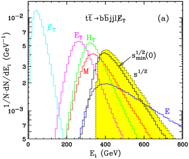
Figure 2: Unit-normalized distributions of the various energy scale variables $E_{i}$ introduced in Section 3: $E$ (blue), $\not\!\!E_{T}$ (cyan), $E_{T}$ (magenta), $H_{T}$ (green), $M$ (red) and $\hat{s}^{1/2}_{min}(0)$ (black); in (a) single-lepton and (b) dilepton $t\bar{t}$ events. The dotted (yellow-shaded) histograms are identical in panels (a) and (b) and show the true $\hat{s}^{1/2}$ distribution.

We shall illustrate our comparisons with specific examples, illustrated in Figs. 2, 3 and 4. In each case, we shall plot the six different global inclusive variables $E_{i}$ introduced so far, with the following color scheme: in Figs. 2-4 we shall plot the calorimeter energy $E$ (15) with blue lines, the missing transverse energy $\not\!\!E_{T}$ (3) with cyan lines, the total transverse energy $E_{T}$ (19) with magenta lines, the $H_{T}$ variable (20) with green lines, the total visible mass $M$ (21) with red lines, and finally, our $\hat{s}^{1/2}_{min}(0)$ variable (23) with solid black lines. All numerical results shown here have been obtained with PYTHIA [57] and the PGS detector simulation package [58]. As our first example, shown in Fig. 2, we choose $t\bar{t}$ production at the LHC (the corresponding data from the Tevatron already exists, so the same comparison can also be made directly with CDF and D0 data as well). In Fig. 2(a) (Fig. 2(b)) we show our results for the semi-leptonic (dilepton) channel. The dilepton $t\bar{t}$ sample is rather similar to a hypothetical new physics signal due to dark matter particle production: each event has a certain amount of missing energy, which is due to two invisible particles escaping the detector.

In each panel of Fig. 2, the dotted (yellow-shaded) histogram shows the true $\hat{s}^{1/2}$ distribution, which is the one we would ideally want to measure. However, due to the missing neutrinos, $\hat{s}^{1/2}$ is not directly observable, unless we make some further assumptions and attempt some kinematical event reconstruction. Therefore we concentrate on the remaining distributions shown in Fig. 2, which are immediately and directly observable. In particular, we shall pose the question, which among the various distributions exhibited in Fig. 2 seems to be the best approximation to the true $\hat{s}^{1/2}$ distribution. A quick glance at Fig. 2 reveals that the variable which comes closest to the true $\hat{s}^{1/2}$ is precisely our variable $\hat{s}^{1/2}_{min}(0)$ defined in (23). As for the rest, we see that the missing transverse energy $\not\!\!E_{T}$ is a very poor estimator of the energy scale of the events, while $E_{T}$, $H_{T}$ and $M$ are doing a little bit better, yet are still quite far off. As can be expected from its definition (20), $H_{T}$ is always somewhat larger than $E_{T}$, while $H_{T}$ and $M$ are rather similar, with $H_{T}$ ($M$) doing better for the dilepton (semi-leptonic) case. Finally, the total energy $E$ is relatively close to the true $\hat{s}^{1/2}$ distribution, but is quite broad in both Figs. 2(a) and 2(b). In contrast, the $\hat{s}^{1/2}_{min}(0)$ distribution is quite sharp, and is thus a better indicator of the relevant energy scale.

Let us now take a closer look at the two $\hat{s}^{1/2}$ distributions in each panel of Fig. 2. Since $\hat{s}^{1/2}_{min}$ was defined through a minimization procedure, it is clear that it will always underestimate the true $\hat{s}^{1/2}$. Fig. 2 quantifies the amount of this underestimation for the case of $t\bar{t}$ events. We see that $\hat{s}^{1/2}_{min}(0)$ is tracking the true $\hat{s}^{1/2}$ quite well for the case of semi-leptonic $t\bar{t}$ events in Fig. 2(a). This could have been expected on very general grounds: for semi-leptonic events, we are missing a single neutrino, whose transverse momentum is actually measured through $\not\!\!\vec{P}_{T}$, so that the only mistake we are making in approximating $\hat{s}^{1/2}\approx\hat{s}^{1/2}_{min}(0)$ is due to the unknown longitudinal component $p_{1z}$. In the case of dilepton events, however, there are two missing neutrinos, and thus more unknown degrees of freedom which we have to fix rather ad hoc according to our prescription (9, 10). The resulting error is larger and leads to a larger displacement between the true $\hat{s}^{1/2}$ distribution and its $\hat{s}^{1/2}_{min}(0)$ approximation, as can be seen in Fig. 2(b).

In the case of $t\bar{t}$ illustrated in Fig. 2 the missing energy arises from massless SM neutrinos, so that the approximation $M_{inv}=0$ is well justified. Let us now consider a situation where the observed missing energy signal is due to massive neutral stable particles, as opposed to SM neutrinos. The prototypical example of this sort is low energy supersymmetry with conserved $R$-parity, and this is what we shall use for our next two examples as well. Each SUSY event will be initiated by the pair-production of two superpartners, which will then cascade decay to the lightest supersymmetric particle (LSP), which we shall assume to be the lightest neutralino $\tilde{\chi}^{0}_{1}$. Since there are two SUSY cascades per event, there will be two LSP particles in the final state, so that

$$n_{inv}=n_{\chi}=2\ .$$ (24)

Furthermore, since the two LSPs are identical, we also have

$$m_{1}=m_{2}\equiv m_{\chi}\ ,$$ (25)

i.e. in what follows we shall denote the true LSP mass with $m_{\chi}$. From (5), (24) and (25) it follows that the true total invisible mass in any SUSY event is simply

$$M_{inv}=2m_{\chi}\ .$$ (26)

However, the true LSP mass $m_{\chi}$ is a priori unknown, therefore, when we construct our variable

$$\hat{s}^{1/2}_{min}(M_{inv})=\hat{s}^{1/2}_{min}(2m_{\chi})$$ (27)

for the SUSY examples, we will have to make a guess for the value of the LSP mass $m_{\chi}$. We shall denote this trial value by $\tilde{m}_{\chi}$, in order to distinguish it from the true LSP mass $m_{\chi}$. This situation is reminiscent of the case of the Cambridge $M_{T2}$ variable [9], where in order to construct the $M_{T2}$ variable itself, one must first choose a test value for the LSP mass. Our notation here is consistent with the notation for $M_{T2}$ used in [54].

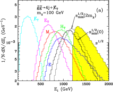
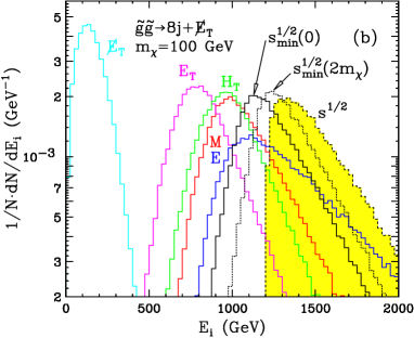
Figure 3: The same as Fig. 2, but for gluino pair production events with (a) 2-jet gluino decays as in (28) and (b) 4-jet gluino decays as in (29). The SUSY masses are fixed as follows: $m_{\tilde{\chi}^{0}_{1}}=100$ GeV, $m_{\tilde{\chi}^{0}_{2}}=200$ GeV and $m_{\tilde{g}}=600$ GeV. In addition to the variables shown in Fig. 2, here we also plot the $\hat{s}^{1/2}_{min}(2m_{\chi})$ distribution (dotted line) with the correct value of the invisible mass $M_{inv}=2m_{\chi}=2m_{\tilde{\chi}^{0}_{1}}$.

We are now ready to describe our SUSY examples. For our study we will choose a rather difficult signature — jets plus $\not\!\!E_{T}$, for which all other proposed methods for mass determination are bound to face significant challenges. For concreteness, we consider gluino production, followed by a gluino decay to jets and a neutralino. In Fig. 3 we consider gluino pair-production ($\tilde{g}\tilde{g}$), while in Fig. 4 we show results for associated gluino-LSP production ($\tilde{g}\tilde{\chi}^{0}_{1}$). In addition, we consider two different possibilities for the gluino decays. The first case, shown in Figs. 3(a) and Figs. 4(a), has the gluino decaying directly to the LSP:

$$\tilde{g}\to jj\tilde{\chi}^{0}_{1}\ ,$$ (28)

so that the gluino pair-production events in Fig. 3(a) have 4 jets and missing energy, while the associated gluino-LSP production events in Fig. 4(a) have two jets and missing energy. In the second case, presented in Figs. 3(b) and Figs. 4(b), we forced the gluino to always decay to $\tilde{\chi}^{0}_{2}$, which in turn decays via a 3-body decay to 2 jets and the LSP:

$$\tilde{g}\to jj\tilde{\chi}^{0}_{2}\to jjjj\tilde{\chi}^{0}_{1}\ .$$ (29)

As a result, the gluino pair-production events in Fig. 3(b) will exhibit 8 jets and missing energy, while the associated gluino-LSP production events in Fig. 4(b) will have four jets and missing energy. Of course, the actual number of reconstructed jets in such events may be even higher, due to the effects of initial state radiation (ISR) and/or jet fragmentation. In any case, such multijet events will be very challenging for any exclusive reconstruction method, therefore it is interesting to see what we can learn about them from the global inclusive variables discussed here.

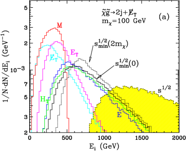
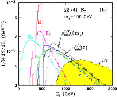
Figure 4: The same as Fig. 3, but for events of associated gluino-LSP production.

For concreteness, in what follows we shall always fix the relevant SUSY masses according to the approximate gaugino unification relation

$$m_{\tilde{g}}=3m_{\tilde{\chi}^{0}_{2}}=6m_{\tilde{\chi}^{0}_{1}}\equiv 6m_{\chi}\ ,$$ (30)

and since we assume three-body decays in (28) and (29), we do not need to specify the SUSY scalar mass parameters, which can be taken to be very large. In addition, as implied by (30), we imagine that the lightest two neutralinos are gaugino-like, so that we do not have to specify the higgsino mass parameter either, and it can be taken to be very large as well.

Fig. 3 shows our results for the different global inclusive variables introduced earlier, for the case of gluino pair-production. All in all, the outcome is not too different from what we found previously in Fig. 2 for the $t\bar{t}$ case: when it comes to approximating the true $\hat{s}^{1/2}$ distribution, the missing energy $\not\!\!E_{T}$ does the worst, our variable $\hat{s}^{1/2}_{min}(0)$ does the best, and all other remaining variables are somewhere in between those two extremes. This time, in Fig. 3 we also plot one “cheater” distribution, namely $\hat{s}^{1/2}_{min}(2m_{\chi})$, where we have used the correct value of the invisible mass $M_{inv}=2m_{\chi}=2m_{\tilde{\chi}^{0}_{1}}$. It demonstrates that knowing the actual value of the LSP mass helps (since $\hat{s}^{1/2}_{min}(2m_{\chi})$ gets closer to the truth), but is not crucial: the quantity $\hat{s}^{1/2}_{min}(0)$ still does surprisingly well in approximating the true $\hat{s}^{1/2}$.

Notice that when the missing energy in the data is due to massive BSM particles, there are two sources of error in approximating $\hat{s}^{1/2}\approx\hat{s}^{1/2}_{min}(0)$, each leading to an underestimation. By comparing the three different types of $\hat{s}^{1/2}$ distributions shown in each panel of Fig. 3, one can see quantitatively the effect of each source. First, when we take the minimum possible value of $\hat{s}^{1/2}$ in (8), we are underestimating by a certain amount, which can be seen by comparing the “cheater” distribution $\hat{s}^{1/2}_{min}(2m_{\chi})$ (dotted line) to the $\hat{s}^{1/2}$ truth (yellow shaded). Second, as we do not know a priori the LSP mass, we take conservatively $M_{inv}=0$, which leads to a further underestimation, as evidenced by the difference between the $\hat{s}^{1/2}_{min}(0)$ distribution (solid line) and its “cheater” version $\hat{s}^{1/2}_{min}(2m_{\chi})$. In spite of those two undesirable effects, the $\hat{s}^{1/2}_{min}(0)$ approximation that we end up with is still surprisingly close to the real one, and is certainly the best approximation among the variables we are considering.

The common thread in our first two examples shown in Figs. 2 and 3 was that the events were symmetric, i.e. we produce the same type of particles, which then decay identically on each side of the event. As our last example, we shall consider an extreme version of an asymmetric event, namely one where all visible particles come from the same side of the event, i.e. from a single decay chain. The process of associated gluino-LSP production is exactly of this type - all jets arise from the decay chain of a single gluino, which is recoiling against an LSP. The topology of these events is very different from the events considered earlier in Figs. 2 and 3. Nevertheless, as seen in Fig. 4, we find very similar results. In particular, among all the different global inclusive variables that we are considering, the quantity $\hat{s}^{1/2}_{min}(0)$ is still the one closest to the true $\hat{s}^{1/2}$ distribution.

4 Dependence of $\hat{s}^{1/2}_{min}$ on the unknown masses of invisible particles

In the previous Section 3 we demonstrated the advantage of $\hat{s}^{1/2}_{min}$ in comparison to the other commonly used global inclusive event variables. From now on we shall therefore focus our discussion entirely on $\hat{s}^{1/2}_{min}$ and its properties. In this Section we shall investigate in more detail the dependence of $\hat{s}^{1/2}_{min}$ on the (a priori unknown) masses of the invisible particles which are causing the observed missing energy signal. Then in the next Section 5 we shall use these results to correlate the observed $\hat{s}^{1/2}_{min}$ distribution to the masses of the parent particles which were originally produced in the event.

Recall that in the three examples from the previous section, we always conservatively chose the invisible mass to be zero: $M_{inv}=0$ and we correspondingly considered $\hat{s}^{1/2}_{min}(0)$. This choice is actually a good starting point in studying any missing energy signature by means of $\hat{s}^{1/2}_{min}(M_{inv})$. The assumption of $M_{inv}=0$ is precisely what one would do if one were to assume that the missing energy is simply due to SM neutrinos, as opposed to some new physics. However, if the observed missing energy signal is in excess of the expected SM backgrounds, then an alternative, BSM explanation for those events must be sought. In that case, we would not know the mass of the invisible particles, and we would have to make a guess. Our main goal in this section is to study numerically the effect of this guess. Our philosophy will be to revisit the SUSY examples from Section 3 and simply vary the test mass $\tilde{m}_{\chi}$ of the invisible particles (the LSPs). Since the two LSPs are identical (see eq. (25)), we will take their test masses to be the same as well.

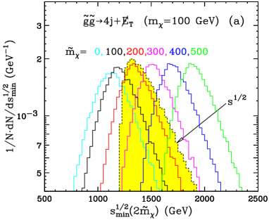
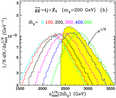
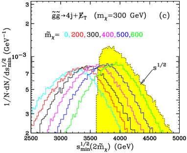
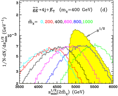
Figure 5: Unit-normalized distributions of the $\hat{s}^{1/2}_{min}(M_{inv})$ variable for several different SUSY mass spectra: (a) $m_{\tilde{\chi}^{0}_{1}}=100$ GeV, (b) $m_{\tilde{\chi}^{0}_{1}}=200$ GeV, (c) $m_{\tilde{\chi}^{0}_{1}}=300$ GeV, and (d) $m_{\tilde{\chi}^{0}_{1}}=400$ GeV. The remaining masses are fixed according to (30). We consider gluino pair-production events with 2-jet gluino decays as in (28). In each panel, we plot the $\hat{s}^{1/2}_{min}(M_{inv})=\hat{s}^{1/2}_{min}(2\tilde{m}_{\chi})$ distributions for several representative values of the trial LSP mass $\tilde{m}_{\chi}$ as shown. The color scheme is such that the black histogram is always the case where we happen to use the correct value of the LSP mass: $\tilde{m}_{\chi}=m_{\chi}$. The dotted (yellow-shaded) histogram gives the true $\hat{s}^{1/2}$ distribution.

Our results are presented in Figs. 5, 6 and 7. In Figs. 5 and 6 we consider gluino pair production. In Fig. 5 each gluino decays to 2 jets as in (28), while in Fig. 6 each gluino decays to 4 jets as in (29). Then in Fig. 7 we consider asymmetric events of associated gluino-LSP production, where the single gluino decays to 4 jets as in (29). In each figure, we consider four different study points, defined through the value of the true LSP mass $m_{\chi}$. In all three Figs. 5-7, panels (a) correspond to $m_{\chi}=100$ GeV, panels (b) have $m_{\chi}=200$ GeV, panels (c) have $m_{\chi}=300$ GeV, while in panels (d) $m_{\chi}=400$ GeV. As before, the remaining masses $m_{\tilde{g}}$ and $m_{\tilde{\chi}^{0}_{2}}$ are always fixed according to the approximate gaugino unification relation (30). Each panel in Figs. 5-7 exhibits the true $\hat{s}^{1/2}$ distribution (yellow-shaded histogram), and the corresponding $\hat{s}^{1/2}_{min}(2\tilde{m}_{\chi})$ distributions for several representative values of the test LSP mass $\tilde{m}_{\chi}$. Each $\hat{s}^{1/2}_{min}$ curve is both color coded and labelled by its corresponding value of $\tilde{m}_{\chi}$. Our color scheme is such that the $\hat{s}^{1/2}_{min}$ histogram in black is the one where we happen to use the correct value of the LSP mass, i.e. when $\tilde{m}_{\chi}=m_{\chi}$.

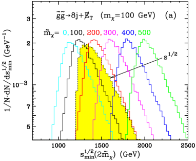
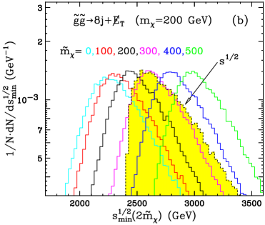
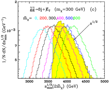
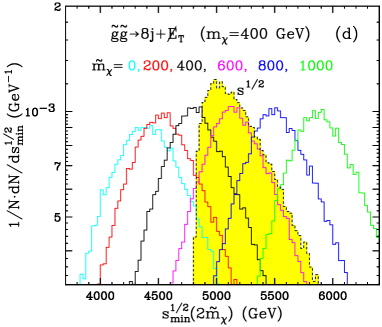
Figure 6: The same as Fig. 5, but for 4-jet gluino decays as in (29).

The qualitative behavior seen in Figs. 5-7 is more or less as expected: the $\hat{s}^{1/2}_{min}(2\tilde{m}_{\chi})$ distributions shift to higher energy scales, as we increase the value of the test mass $\tilde{m}_{\chi}$. This can be easily understood from the definition (14) of the $\hat{s}^{1/2}_{min}(M_{inv})$ variable: for any given set of $E$, $P_{z}$ and $\not\!\!E_{T}$ values, $\hat{s}^{1/2}_{min}(M_{inv})$ is a monotonically increasing function of $M_{inv}$. The shifts observed in Figs. 5-7 also make perfect physical sense: obviously, one needs more energy in order to produce heavier invisible particles.

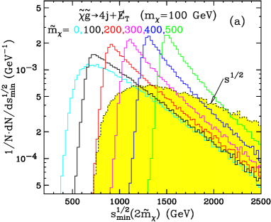
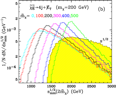
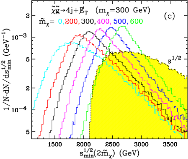
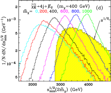
Figure 7: The same as Fig. 6, but for events of associated gluino-LSP production ($\tilde{g}\tilde{\chi}^{0}_{1}$).

Let us now concentrate on the quantitative aspects of Figs. 5-7. Upon careful inspection of the three figures, we notice that when the test mass $\tilde{m}_{\chi}$ is equal to the true mass $m_{\chi}$ (i.e. for the black colored histograms), the corresponding distribution $\hat{s}^{1/2}_{min}(2m_{\chi})$ peaks very close to the true $\hat{s}^{1/2}$ threshold $\left(\hat{s}^{1/2}\right)_{thr}$. As usual, we define the threshold $\left(\hat{s}^{1/2}\right)_{thr}$ as the value where the true $\hat{s}^{1/2}$ distribution (yellow shaded histogram) sharply turns on. This observation is potentially extremely important, since the threshold $\left(\hat{s}^{1/2}\right)_{thr}$ is simply related to the masses of the two particles which were originally produced in the event. For example, for the gluino pair production events in Figs. 5 and 6 the threshold is given by

$$\left(\hat{s}^{1/2}\right)_{thr}=2m_{\tilde{g}}=12m_{\chi}\ ,$$ (31)

where the second equality is valid only under the gaugino unification assumption (30). Similarly, in the case of associated gluino-LSP production in Fig. 7, the threshold is given by

$$\left(\hat{s}^{1/2}\right)_{thr}=m_{\tilde{g}}+m_{\tilde{\chi}^{0}_{1}}=7m_{\chi}\ ,$$ (32)

where once again the second equality is due to our assumption (30). It is easy to verify that in all three figures 5, 6 and 7, the $\hat{s}^{1/2}$ thresholds (i.e. the sharp turn-ons in the yellow-shaded distributions) always occur at the locations predicted in eqs. (31) and (32).

Let us now introduce one last piece of notation. In what follows we shall use the notation

$$\left(\hat{s}^{1/2}_{min}(M_{inv})\right)_{peak}$$ (33)

to denote the particular value of $\hat{s}^{1/2}_{min}$ where we find the peak of the distributions

$$\frac{dN(\hat{s}^{1/2}_{min}(M_{inv}))}{d\hat{s}^{1/2}_{min}}$$ (34)

which are plotted in Figs. 5-7. In other words,

$$\left[\frac{d}{d\hat{s}^{1/2}_{min}}\frac{dN(\hat{s}^{1/2}_{min}(M_{inv}))}{d\hat{s}^{1/2}_{min}}\right]_{\hat{s}^{1/2}_{min}=\left(\hat{s}^{1/2}_{min}(M_{inv})\right)_{peak}}=0.$$ (35)

With those conventions, we can now formulate our empirical observation above as

$$\left(\hat{s}^{1/2}\right)_{thr}\approx\left(\hat{s}^{1/2}_{min}(2m_{\chi})\right)_{peak}\ .$$ (36)

The last equation is one of the main results in this paper. While we were not able to derive it in a strict mathematical sense, it is nevertheless supported by our numerical results shown in Figs. 5-7. We also checked many other SUSY examples, where we used different mass spectra and different production processes and decays. We found that in all cases the approximate relation (36) still holds. Fig. 8 quantifies this statement for the two previously considered processes of gluino pair production and associated gluino-LSP production, where the gluinos are forced to decay either to 2 jets as in (28) or to 4 jets as in (29). In the figure we compare the following three quantities, all of which are related in one way or another to the energy scale $\hat{s}^{1/2}$ of the events:

• $\left(\hat{s}^{1/2}\right)_{ave}$ : this is the average of the true $\hat{s}^{1/2}$ distribution (the one shown in the previous figures with the yellow-shaded histogram). Here we had to pick some variable which would characterize the true $\hat{s}^{1/2}$ distribution. Two alternative choices which we also considered were the peak or the mean of the true $\hat{s}^{1/2}$ distribution. All three of these variables are numerically quite close, with the peak value typically being the lowest, and the average value being the largest. In the end we chose $\left(\hat{s}^{1/2}\right)_{ave}$ for its computational simplicity. This choice is rather inconsequential for our conclusions below, since we are introducing the $\left(\hat{s}^{1/2}\right)_{ave}$ variable only for illustration purposes in Fig. 8. As we shall see, $\left(\hat{s}^{1/2}\right)_{ave}$ actually cancels out in the final comparison between the next two variables.

• $\left(\hat{s}^{1/2}\right)_{thr}$ : this is the threshold of the true $\hat{s}^{1/2}$ distribution, i.e. the minimum allowed value of $\hat{s}^{1/2}$. Since the minimum $\hat{s}^{1/2}$ is obtained when the parent particles are produced at rest, $\left(\hat{s}^{1/2}\right)_{thr}$ is nothing but the sum of the parent particle masses, as indicated in eqs. (31) and (32). Therefore, $\left(\hat{s}^{1/2}\right)_{thr}$ is precisely the parameter that we would like to measure, in order to determine the true mass scale of the parent particles.

• $\left(\hat{s}^{1/2}_{min}(2m_{\chi})\right)_{peak}$ : this is the parameter defined in eq. (35), namely the location of the peak of the $\hat{s}^{1/2}_{min}(2m_{\chi})$ distribution, where we use the correct value for the invisible mass, in this case $M_{inv}=2m_{\chi}$, since each SUSY event has two escaping LSPs.

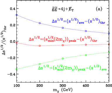
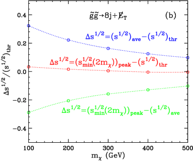
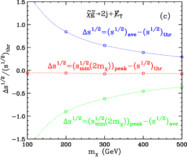
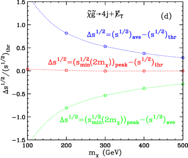
Figure 8: Validity of the approximation (36) as a function of the LSP mass $m_{\chi}$. The SUSY mass spectrum is fixed as in (30). In panels (a) and (b) we consider gluino pair production events, while in panels (c) and (d) we study associated gluino-LSP production. In panels (a) and (c) we force the gluino to decay to 2 jets as in (28), while in panels (b) and (d) each gluino decays to 4 jets as in (29). In each panel we compare the following three quantities: $\left(\hat{s}^{1/2}\right)_{ave}$, which is the average of the true $\hat{s}^{1/2}$ distribution; $\left(\hat{s}^{1/2}\right)_{thr}$, which is the threshold of the true $\hat{s}^{1/2}$ distribution; and $\left(\hat{s}^{1/2}_{min}(2m_{\chi})\right)_{peak}$, which is the location of the peak of the $\hat{s}^{1/2}_{min}(2m_{\chi})$ distribution.

According to our empirically derived conjecture (36), the last two variables are approximately equal, and the purpose of Fig. 8 is to test this hypothesis, using the previously considered SUSY examples: gluino pair production (panels (a) and (b)), and associated gluino-LSP production (panels (c) and (d)). In panels (a) and (c) we force the gluino to decay to 2 jets as in (28), while in panels (b) and (d) each gluino decays to 4 jets as in (29). Each line in Fig. 8 gives the fractional difference between a pair of $\hat{s}^{1/2}$ quantities as defined above. For normalisation we used the value of $\left(\hat{s}^{1/2}\right)_{thr}$, which is given by (31) for panels (a) and (b) and by (32) for panels (c) and (d). We vary the relevant part of the SUSY spectrum by changing the input value of the LSP mass $m_{\chi}$ and adjusting the other masses in accord with (30).

The main result in Fig. 8 is the comparison between the experimentally observable quantity $\left(\hat{s}^{1/2}_{min}(2m_{\chi})\right)_{peak}$ and the theoretical parameter $\left(\hat{s}^{1/2}\right)_{thr}$. As indicated by the red lines in Fig. 8, for the examples shown, those two quantities differ by no more than 10%, thus validating our conjecture (36) at the 10% level as well. We find this result quite intriguing. After all, we have not attempted any event reconstruction or decay chain identification, we are looking at very complex and challenging multijet signatures, and we have even included detector resolution effects. After all those detrimental factors, the possibility of making any kind of statement regarding the mass scale of the new physics at the level of 10% should be considered as rather impressive.

We find it instructive to understand how we ended up with the observed precision, by comparing these two quantities $\left(\hat{s}^{1/2}_{min}(2m_{\chi})\right)_{peak}$ and $\left(\hat{s}^{1/2}\right)_{thr}$ to the true $\hat{s}^{1/2}$ as represented by its average $\left(\hat{s}^{1/2}\right)_{ave}$. The blue lines in Fig. 8 show the fractional difference between $\left(\hat{s}^{1/2}\right)_{ave}$ and $\left(\hat{s}^{1/2}\right)_{thr}$. We see that this difference varies by quite a lot, on the order of 10-30% for gluino pair-production, but may get in excess of 150% for associated gluino-LSP production. As expected, $\left(\hat{s}^{1/2}\right)_{ave}$ is always larger than the threshold value $\left(\hat{s}^{1/2}\right)_{thr}$, since the parent particles are typically produced with some boost, and the blue lines in Fig. 8 simply quantify the effect of this boost.

On the other hand, the green lines in Fig. 8 represent the fractional difference (again normalised to $\left(\hat{s}^{1/2}\right)_{thr}$) between the measurable quantity $\left(\hat{s}^{1/2}_{min}(2m_{\chi})\right)_{peak}$ introduced earlier in eq. (35), and the true energy scale of the events as given by $\left(\hat{s}^{1/2}\right)_{ave}$. We see that this time the fractional difference is negative, which simply reflects the fact that our variable $\hat{s}^{1/2}_{min}$, being defined through a minimization condition, will always underestimate the true energy scale. The interesting fact is that while the blue and green curves in Fig. 8 have opposite signs, in absolute value they are very similar, leading to a fortuitous cancellation. The resulting discrepancy indicated by the red lines is therefore much smaller than either of the two individual errors indicated by the blue and green lines.

It is now easy to understand qualitatively the origin of the approximate relation (36). Due to the boost at production, the true energy scale $\hat{s}^{1/2}$ is larger than the threshold energy $\left(\hat{s}^{1/2}\right)_{thr}$ by a certain amount. Later on, when we approximate $\hat{s}^{1/2}$ with $\hat{s}^{1/2}_{min}$, we underestimate the true energy scale $\hat{s}^{1/2}$ by more or less the same amount, bringing us back near the threshold $\left(\hat{s}^{1/2}\right)_{thr}$. As a result, the $\hat{s}^{1/2}_{min}$ distribution peaks very near the mass threshold $\left(\hat{s}^{1/2}\right)_{thr}$ which we are trying to measure in the first place. Of course, the proximity of the $\hat{s}^{1/2}_{min}$ peak to the threshold $\left(\hat{s}^{1/2}\right)_{thr}$ will be process dependent, but according to the examples considered here, holds to a remarkable accuracy.

5 Correlation of the $\hat{s}^{1/2}_{min}$ peak with the heavy particle mass threshold

In the absence of a rigorous mathematical derivation, eq. (36) should be considered simply as a conjecture. Nevertheless, once eq. (36) is assumed to be approximately true, it allows us to measure the mass scale of the parent particles in terms of the hypothesized test mass $\tilde{m}_{\chi}$ of the lightest invisible particle, e.g. the LSP in SUSY. For example, in the case of gluino pair-production in SUSY, we can use eqs. (31) and (36) to obtain a measurement of the gluino mass

$$\tilde{m}_{\tilde{g}}(\tilde{m}_{\chi})\approx\frac{1}{2}\left(\hat{s}^{1/2}_{min}(2\tilde{m}_{\chi})\right)_{peak}$$ (37)

as a function of the trial LSP mass $\tilde{m}_{\chi}$. Similarly, we can measure the gluino mass even in the much more challenging case of associated gluino-LSP production: from eqs. (32) and (36), we obtain

$$\tilde{m}_{\tilde{g}}(\tilde{m}_{\chi})\approx\left(\hat{s}^{1/2}_{min}(2\tilde{m}_{\chi})\right)_{peak}-\tilde{m}_{\chi}\ .$$ (38)

As evidenced from eqs. (37) and (38), these measurements are very straightforward, since the only experimental input needed for them is the location of the peak of our all-inclusive global variable $\hat{s}^{1/2}_{min}$. One should not be bothered by the fact that we did not get an absolute measurement of the gluino mass, but only obtain it as a function of the LSP mass. This is a well-known drawback of the other common mass measurement methods as well. For example, the classic $M_{T2}$ endpoint analysis only yields the heavier parent mass as a function of the lighter child mass [9]. Similarly, the measurement of a single endpoint in some observable invariant mass distribution provides only a single functional relation between the masses of the intermediate particles in the decay chain, and by itself does not measure the absolute scale. In this sense, our measurement (37) is on equal footing with the more traditional methods.

However, it is worth emphasizing the advantage of our method in the case of asymmetric events, where the parent particles are very different. An extreme version of such events is provided by the associated gluino-LSP production considered earlier. Under those circumstances, the standard $M_{T2}$ method does not apply, while the single decay chain in the event may prove to be too short or too messy to provide a clean measurement through the invariant mass endpoint method. In contrast, we can still utilize $\hat{s}^{1/2}_{min}$ for the measurement indicated in (38) and a corresponding gluino mass determination.

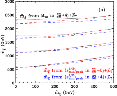
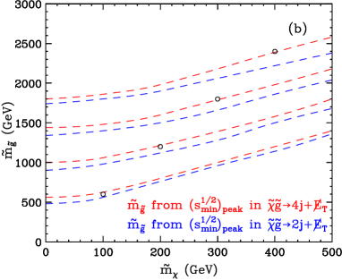
Figure 9: The correlation between the test LSP mass $\tilde{m}_{\chi}$ and the corresponding gluino mass $\tilde{m}_{\tilde{g}}$, derived from (a) our proposed measurement (37) in gluino pair-production events, or (b) our proposed measurement (38) in associated gluino-LSP production events. Red (blue) lines correspond to the case of gluino decays to 4 jets as in (29) (gluino decays to 2 jets as in (28)). The black dotted lines in panel (a) indicate the theoretically derived correlation from an ideal $M_{T2}$ endpoint analysis, i.e. assuming perfect resolution of the jet combinatorial ambiguity and ignoring any detector smearing. The open circles mark the locations of the true masses $(m_{\chi},m_{\tilde{g}})$, for each of our four study points.

Let us now see how well the proposed measurements (37) and (38) will do for each of the SUSY examples considered in the previous section. In Fig. 9(a) we used eq. (37) to convert our previous measurements of the various $\hat{s}^{1/2}_{min}(2\tilde{m}_{\chi})$ peaks in Figs. 5 and 6 into a corresponding gluino mass measurement. The red (blue) dashed lines correspond to the case of 4-jet (2-jet) gluino decays as in (29) ((28)). We show results for the same four study points used in the four panels of Figs. 5 and 6, and the open circles mark the locations of the true masses $(m_{\chi},m_{\tilde{g}})$, for each study point.

The quality of the measurement (37) can be judged from the proximity of the experimentally derived $\tilde{m}_{\tilde{g}}(\tilde{m}_{\chi})$ curves shown in the figure to the exact location of the true masses $(m_{\chi},m_{\tilde{g}})$. We see that both the red and blue curves in Fig. 9(a) pass very close to the true answer, especially for the study points with lower $m_{\chi}$. In fact, we obtain a better measurement from the more complex 8-jet events (the red curves). At first sight, this may seem counterintuitive, until one realizes that the more visible objects are present in the event, the smaller the effect of the missing particles, and hence the smaller the error due to our approximation (9, 10). Such multijet events appear very challenging to be tackled by any other means. For the sake of comparison, the black dotted lines in Fig. 9(a) show the theoretically derived correlation from an ideal $M_{T2}$ endpoint analysis, i.e. assuming perfect resolution of the jet combinatorial ambiguity and ignoring any detector resolution effects. Comparing the red line from our measurement (37) to the ideal $M_{T2}$ line, we are tempted to conclude that, in essence, our $\hat{s}^{1/2}_{min}$ variable contains pretty much the same amount of information as $M_{T2}$. The big advantage of $\hat{s}^{1/2}_{min}$, however, is the fact that we can obtain this information at a much lower cost in terms of analysis effort.

Finally, in Fig. 9(b) we show our results from the analogous measurement (38) in the case of associated gluino-LSP production. Here we also consider two different options for the gluino decay — 2 jet decays as in (28) (blue lines), or 4 jet decays as in (29) (red lines). We then plot the resulting functional dependence $\tilde{m}_{\tilde{g}}(\tilde{m}_{\chi})$ for each of the four study points considered earlier. Comparing Fig. 9(b) to Fig. 9(a) which we just discussed, we arrive at very similar conclusions: the measurement (38) is still quite accurate, and the superior result is provided by the more complex topology. Notice that here we do not show any $M_{T2}$-based results, since the concept of $M_{T2}$ can not be applied to an extremely asymmetric topology like this one.

6 The impact of initial state radiation and multiple parton interactions

Up to now we have been discussing the $\sqrt{\hat{s}}$ variable of the primary parton-level hard scattering (HS). In principle, $\sqrt{\hat{s}}$ can be measured exactly, whenever we could both detect and identify the decay products of the heavy particles which were initially produced in the HS. Unfortunately, in reality it is rather difficult to measure $\sqrt{\hat{s}}$ directly, for a couple of reasons:

1. Omitting relevant particles from the $\sqrt{\hat{s}}$ calculation. This case arises whenever some of the decay products resulting from the HS are not detected. For example, this may happen due to the imperfect hermeticity of the detector, where some of the relevant decay products are lost down the beam pipe. Fortunately, in reality this effect is pretty small. A much more serious problem arises whenever there are invisible particles $\chi_{i}$ (see Fig. 1) among the relevant decay products. Then, a relatively large fraction of the initial $\sqrt{\hat{s}}$ may go undetected, as can be seen by comparing the $\sqrt{\hat{s}}_{min}$ distributions in Figs. 3-7 to the respective true (yellow-shaded) $\sqrt{\hat{s}}$ distributions.

2. Including irrelevant particles in the $\sqrt{\hat{s}}$ calculation. In general, any given event will contain a certain number of particles which will be seen in the detector, but did not originate from the primary HS. Initial state radiation (ISR), multiple parton interactions (MPI) and pile-up are the main examples of processes contributing to this effect. The pile-up effect can be controlled by a suitable $\Delta z$ cut, removing from consideration tracks which do not appear to originate from the primary vertex. However, ISR and MPI can be a serious problem. Including the extra particles will necessarily lead to an increase in the measured value of $\sqrt{\hat{s}}$. In order to emphasize this difference, in the rest of this section we shall be using a prime to designate the experimentally measured quantities which include the full ISR and MPI effects ($\sqrt{{\hat{s}}^{\prime}}$ and $\sqrt{{\hat{s}}^{\prime}}_{min}$, correspondingly).

Our proposal for dealing with the first of these two problems was to introduce the $\sqrt{\hat{s}}_{min}$ variable in lieu of the true $\sqrt{\hat{s}}$. We then found an interesting empirical correlation (36) between $\sqrt{\hat{s}}_{min}(2m_{\chi})$ and the new physics mass scale. Now we shall turn our attention to dealing with the second problem, namely the fact that $\sqrt{{\hat{s}}^{\prime}}_{min}>\sqrt{\hat{s}}_{min}$.

Before we begin, we should mention that, depending on the particular circumstances and/or the goal of the experimenter, there may be certain situations where the inequality $\sqrt{{\hat{s}}^{\prime}}_{min}>\sqrt{\hat{s}}_{min}$ may not represent an actual problem. For example, if one is simply trying to measure the total energy in the observed events and not just the energy of the HS, then for missing energy events the relevant quantity of interest would be $\sqrt{{\hat{s}}^{\prime}}_{min}$ itself, which would still be given by the expression (4) derived in Section 2. There may also be situations where the ISR and/or MPI products may be reliably identified and excluded from the $\sqrt{\hat{s}}_{min}$ calculation. For example, consider a lepton collider and a missing energy signature with any number of jets and/or leptons. Since MPI is absent, while ISR and beamstrahlung would only contribute photons, there will be no confusion with regards to which particles are due to ISR and which are coming from the HS. The analogous example at hadron colliders would be a signature containing anything but QCD jets. In what follows we shall ignore such trivial cases and instead focus on the much more challenging case of hadron colliders and jetty signatures, where the ISR/MPI products cannot be easily recognized.

In the absence of any reliable methods for resolving the jet combinatorial problem on an event by event basis, one is left with two options. First, one may try to compensate for the ISR/MPI effects on the global $\sqrt{{\hat{s}}^{\prime}}_{min}$ distribution. In order to do this, one needs to know how ISR/MPI would affect the original $\sqrt{\hat{s}}_{min}$ distribution. Ideally, this information should be measured from real data, using some Standard Model process as a standard candle. For example, Drell-Yan can provide the relevant information for a $q\bar{q}$ initial state [59], while $t\bar{t}$ can be used to study the $gg$ initial state. Alternatively, one may calculate the ISR effects from first principles in QCD. Both of these approaches will be pursued in a future work [60].

A second approach would be to design and apply cuts which would minimize the ISR and MPI effects on the calculation of $\sqrt{{\hat{s}}^{\prime}}_{min}$. Unfortunately, this is rather difficult to do in a model-independent fashion, since the size of the ISR effect is very model-dependent and depends on many factors: the energy of the collider (Tevatron or LHC), the mass of the produced particles, the identity of the partons initiating the HS, etc. Therefore, the optimal method to compensate for the ISR effect will also depend on all of these factors and will need to be decided on a case by case basis.

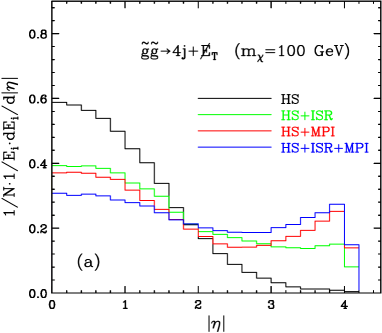
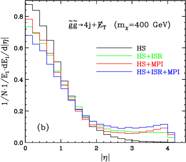
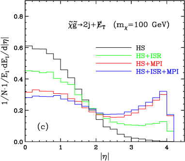
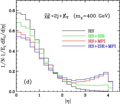
Figure 10: Energy distributions as a function of $|\eta|$, for some of the SUSY examples considered earlier: 2-jet gluino decays from gluino pair production with (a) $m_{\chi}=100$ GeV or (b) $m_{\chi}=400$ GeV; and from associated gluino-LSP production with (c) $m_{\chi}=100$ GeV or (d) $m_{\chi}=400$ GeV. The color scheme is such that the black histograms correspond to our previous results from Section 4 in the idealised case without ISR or MPI, while the green (red, blue) histograms include the effect of ISR (MPI, both ISR and MPI). Here $E_{i}$ is the total energy measured in the $i$-th event, and $N$ is the total number of events. As a result, all distributions shown in the figure are unit-normalized.

For the purposes of the current study, we shall use a simple cut-based approach as discussed here, postponing the more complete treatment for [60]. To this end, we need to identify some global property of the ISR and MPI products which would distinguish them from the HS. Since it is well known that ISR and MPI peak in the forward region, it is natural to consider the pseudorapidity $\eta$ as a simple cut variable. The energy distributions as a function of $|\eta|$, for a few representative cases are shown in Fig. 10. We again consider the processes of gluino pair production (Figs. 10(a) and 10(b)) and associated gluino-LSP production (Figs. 10(c) and 10(d)). In each case, the gluino decays to 2 jets as in (28). We choose to show the two extreme cases for the mass spectrum considered earlier: $m_{\chi}=100$ GeV (Figs. 10(a) and 10(c)) and $m_{\chi}=400$ GeV (Figs. 10(b) and 10(d)). The gluino mass is still fixed according to the gaugino unification relation (30). The black histograms in Fig. 10 represent our previous results from Section 4 without any ISR or MPI effects, while the green (red) histograms include the effect of ISR (MPI). Finally, the blue histograms include both the ISR and MPI effects. The plots in Fig. 10 are normalized as follows. For each event, say the $i$-th one, we add the energy deposits in all calorimeter towers at a given $|\eta|$, then divide the sum by the total energy $E_{i}$ observed in the $i$-th event and the total number of events $N$, and finally enter the result into the corresponding $|\eta|$ bin. It is easy to see that this ensures that the final distributions are unit-normalized.

Fig. 10 shows that, as expected, the ISR and MPI effects appear mostly in the forward region. Therefore, by applying a simple $|\eta|<\eta_{max}$ cut, we could reduce their impact. Of course any such rapidity cut would essentially bring us back closer to the transverse quantities from which we were trying to escape from the very beginning. Furthermore, such a simple-minded procedure would introduce an uncontrollable systematic error, which would have to be estimated on a case by case basis. For example, Fig. 10(b) shows that when the spectrum is rather heavy, the ISR/MPI effects are relatively small and can probably be safely neglected altogether, while Figs. 10(a), 10(c) and 10(d) reveal a significant ISR/MPI pollution for a light SUSY spectrum. One should also keep in mind that our conjecture (36) is already subject to a certain systematic error, whose size sets the benchmark for the ISR/MPI elimination study. With those caveats, we choose our cut at $\eta_{max}=1.4$, which is nothing but the end of the barrel and beginning of HE/HF calorimeters in CMS. This choice makes good sense from an experimentalist’s point of view, since the segmentation and performance of the HE/HF calorimeters are relatively worse to begin with.

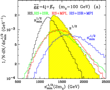
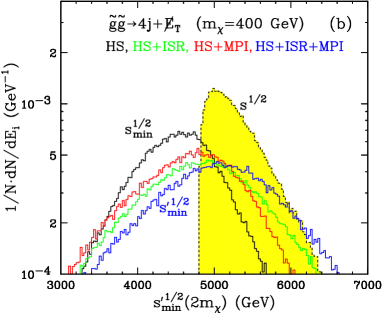
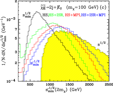
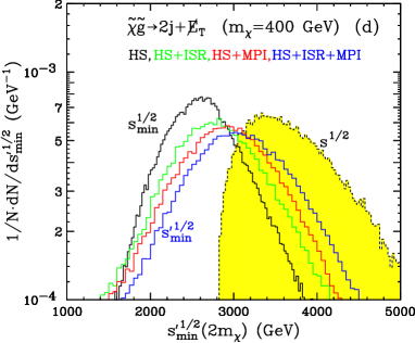
Figure 11: Unit-normalized distributions of $\sqrt{{\hat{s}}}_{min}(2m_{\chi})$ and $\sqrt{{\hat{s}}^{\prime}}_{min}(2m_{\chi})$ for the SUSY examples considered in Fig. 10. The color scheme is the same as in Fig. 10. The blue histograms include both the ISR and MPI effects, and represent the actually measured $\sqrt{\hat{s}^{\prime}}_{min}(2m_{\chi})$, while the green (red) histograms include the effects of ISR (MPI) only. All three of those distributions are subject to the $|\eta|<1.4$ cut discussed in the text. For comparison, we also show our previous results from Section 4, corresponding to the HS only (without any ISR or MPI effects) and without an $\eta$ cut. In particular, the black solid histograms in Fig. 11 represent our previous results for the quantity $\sqrt{\hat{s}}_{min}(2m_{\chi})$, while the black dotted (yellow-shaded) histograms give the true $\hat{s}^{1/2}$ distribution, whose threshold is the parameter to be measured.

Let us now revisit some of the $\sqrt{\hat{s}}_{min}$ distributions from Section 4 and incorporate successively the effects of ISR and/or MPI. Fig. 11 shows our results for the same four SUSY examples from Fig. 10. The green (red) histograms include the effect of ISR (MPI) alone, while the blue histograms include both the ISR and MPI effects, and thus represent the true measured quantity $\sqrt{\hat{s}^{\prime}}_{min}(2m_{\chi})$. All three of those distributions are subject to our $|\eta|<1.4$ cut. For comparison, we also show our previous results from Section 4, corresponding to the HS only (without any ISR or MPI effects) and without an $\eta$ cut. In particular, the black solid histograms in Fig. 11 represent our previous results for the quantity $\sqrt{\hat{s}}_{min}(2m_{\chi})$, while the black dotted (yellow-shaded) histograms give the true $\hat{s}^{1/2}$ distribution, whose threshold is the parameter that ideally we would like to measure.

Fig. 11 confirms that the ISR and MPI effects shift the original HS distribution $\sqrt{\hat{s}}_{min}$ (black histograms) into a harder $\sqrt{\hat{s}^{\prime}}_{min}$ distribution (blue histograms), even after applying the $\eta$ cut. The size of this effect depends on the mass spectrum: it is more pronounced when the spectrum is light, as in Figs. 11(a), 11(c) and 11(d). In the worst case scenario of Fig. 11(c) the location of the $s^{1/2}_{min}$ peak shifts by almost a factor of two. On the other hand, for the best-case scenario of Fig. 11(b) the shift is rather small. By comparing the green and red histograms, we can also deduce the relative importance of ISR versus MPI. We see that the two effects are roughly comparable in size, but as a rule, the red histograms are shifted further along, which suggests that MPI has a somewhat higher impact than ISR, indicating the importance of understanding the full structure of the underlying event at the LHC. The general conclusion from Fig. 11 is that our mass measurement method proposed in Section 4 is likely to work much better if the new particle spectrum happens to be relatively heavy. This assumption is not unreasonable: if the new physics spectrum were too light, then it might have already been ruled out directly or indirectly, and if not, then due to the higher production cross-sections, there should at least be sufficient statistics to attempt some sort of exclusive reconstruction. In this sense, for the case where $\sqrt{\hat{s}}_{min}$ is most likely to be useful, ISR and MPI are least likely to be a problem.

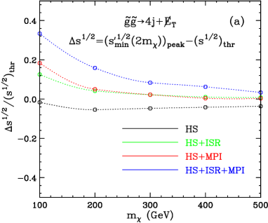
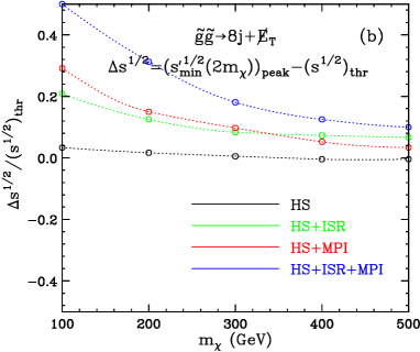
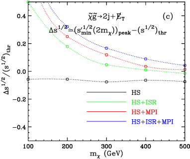
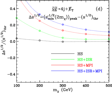
Figure 12: The same as Fig. 8, but including the effects of ISR (green), MPI (red), both ISR and MPI (blue). The variable ${\hat{s}^{\prime}{}}^{1/2}_{\!\!min}(2m_{\chi})$ here is calculated with a cut of $|\eta|<1.4$, corresponding to the coverage of the CMS barrel calorimeter only.

We are now in a position to repeat our mass measurement analysis from Section 5, with the inclusion of ISR and MPI, while ignoring the forward calorimetry through an $|\eta|<1.4$ cut. Our results are shown in Fig. 12. Comparing Figs. 8 and 12, we see that the inclusion of ISR/MPI deteriorates the mass measurement, most notably for light SUSY mass spectra with $m_{\chi}\sim 100-200$ GeV. This should not be surprising, given what we have already seen in Figs. 10 and 11. Nevertheless, for heavier SUSY spectra the precision remains relatively good, typically on the order of $10\%$, even for the most challenging cases of associated gluino-LSP production.

7 Summary and conclusions

Anticipating that an early (late) discovery of a missing energy signal at the LHC (Tevatron) may involve a signal topology which is too complex for a successful and immediate exclusive event reconstruction, we proposed a new global and inclusive variable $\hat{s}^{1/2}_{min}$, defined as follows: it is the minimum required center-of-mass energy, given the measured values of the total calorimeter energy E, total visible momentum $\vec{P}$, and/or missing transverse energy $\not\!\!E_{T}$ in the event. Our variable has several desirable features:

• It is global in the sense that it uses all of the available information in the event and not just transverse quantities, for example.

• It is inclusive in the sense that it does not depend on the specific production process, or particular decay chain. Consequently, it is also very model-independent and does not require any exclusive event reconstruction, which may be a great advantage in the early days of the LHC.

• It is theoretically well defined and as such has a clear physical meaning: it gives the minimum total energy which is consistent with a given observed event. This intuitively clear physical picture allowed us to correlate it with the mass threshold of the new particles as in eq. (36), which turned out to work surprisingly well. In contrast, it is generally difficult to correlate a bump in a purely transverse quantity like $\not\!\!E_{T}$ or $H_{T}$ to any physical mass parameter in a model-independent fashion.

In Section 2 we derived a simple formula (4) for $\hat{s}^{1/2}_{min}$ in terms of the measured $E$, $P_{z}$ and $\not\!\!E_{T}$. The formula is in fact completely general, and is valid for any generic event shown in Fig. 1, with an arbitrary number and/or types of missing particles. Therefore, it can be applied equally successfully to SM as well as BSM missing energy signals.

In Sections 3 and 4 we identified two useful properties of the $\hat{s}^{1/2}_{min}$ variable. First, its shape matches the true $\hat{s}^{1/2}$ distribution better than any of the other global inclusive quantities which are commonly discussed in the literature. More importantly, when we create the $\hat{s}^{1/2}(M_{inv})$ distribution with the true value of the invisible mass $M_{inv}$, its peak is very close to the mass threshold of the parent particles originally produced in the event. This conjecture, summarized in eq. (36), allows us to obtain a rough estimate of the new physics mass scale, as a function of the single parameter $M_{inv}$. For example, in $R$-parity conserving supersymmetry, where $M_{inv}=2m_{\chi}$, we derive a relation between the heavy superpartner mass and the mass of the LSP, as shown in Fig. 9.

Before we conclude, we should comment on several other potential uses of the $\hat{s}^{1/2}_{min}$ variable. Before we even get to the discovery stage, $\hat{s}^{1/2}_{min}(0)$ can already be used for background rejection and increasing signal to noise, just like $M_{T2}(0)$ [25]. In particular, it is interesting to explore the correlations between $\hat{s}^{1/2}_{min}$ and the other global inclusive variables discussed in Section 3 [61]. While we did not include any SM backgrounds in our SUSY plots, we expect that the presence of SM backgrounds will not affect either the existence or the location of the new physics $\hat{s}^{1/2}_{min}(0)$ peak. At large values of $\hat{s}^{1/2}_{min}(0)$, where a new physics signal is most likely to appear, any SM background will be rather smooth and featureless, so that it can be safely subtracted away through a side-band method.

Another possible application of $\hat{s}^{1/2}_{min}(0)$ is at the trigger level. In Section 3 we already saw that $\hat{s}^{1/2}_{min}(0)$ is superior to both $H_{T}$ and $\not\!\!E_{T}$ in identifying the scale of the hard scattering. At the same time, there exist dedicated $H_{T}$ and $\not\!\!E_{T}$ triggers, motivated by the sensitivity of those variables to the relevant energy scale. Given that our variable is doing an even better job in this respect, we believe that the implementation of a high-level $\hat{s}^{1/2}_{min}(0)$ trigger should be given a serious consideration.

As we have been emphasizing throughout, a major advantage of $\hat{s}^{1/2}_{min}$ is that it does not require any explicit event reconstruction and thus it is very model-independent. We should mention that to some extent, these properties are also shared by the $M_{TGen}$ variable proposed in [33]. In calculating $M_{TGen}$, one considers all possible partitions of the visible particles $X_{i}$ in the event, thus effectively eliminating the model-dependence which stems from assuming a particular topology. While $M_{TGen}$ and $\hat{s}^{1/2}_{min}$ are similar in this respect, we believe that $\hat{s}^{1/2}_{min}$ has three definite advantages — first, it is much, much easier to construct. Second, $\hat{s}^{1/2}_{min}$ can be applied to extreme asymmetric topologies where the second side of the event yields no visible particles. A simple example of this sort was the associated gluino-LSP production considered in Figs. 4, 7, 8(c,d), 9(b) and 12(c,d). Finally, the interpretation of $\hat{s}^{1/2}_{min}$ involves reading off a peak, while $M_{TGen}$ requires reading off an endpoint. The former is much easier than the latter: for example, a peak would still be recognizable in the presence of large backgrounds. In contrast, an $M_{TGen}$ endpoint can fade out due to a number of reasons, including detector resolution, combinatorial background, etc. On the other hand, $M_{TGen}$ (and more generally, the $M_{T2}$ class of variables) is better behaved in the presence of ISR. More specifically, the endpoints of the $M_{TGen}$ and $M_{T2}$ distributions in general do shift in the presence of ISR, and their explicit dependence on the “upstream” transverse momentum has to be calculated on a case by case basis [54]. However, the nice feature of both $M_{TGen}$ and $M_{T2}$ is that when the test mass $\tilde{m}_{\chi}$ becomes equal to its true value $m_{\chi}$, there is no such shift and the endpoint remains intact even in the presence of arbitrary ISR. In contrast, as discussed in Section 6, $\hat{s}^{1/2}_{min}$ is always affected by ISR to some extent, requiring some sort of correction.

In conclusion, we reiterate that perhaps the most important advantage of $\hat{s}^{1/2}_{min}$ is that it is readily available from day one. We are therefore eagerly looking forward to the first $\hat{s}^{1/2}_{min}$ plots produced with real LHC data.

List of figures

1. 1 The generic event topology under consideration in this paper. Black (red) lines correspond to SM (BSM) particles. The solid lines denote SM particles $X_{i}$, $i=1,2,\ldots,n_{vis}$, which are visible in the detector, e.g. jets, electrons, muons and photons. The SM particles may originate either from initial state radiation (ISR), or from the hard scattering and subsequent cascade decays (indicated with the green-shaded ellipse). The dashed lines denote neutral stable particles $\chi_{i}$, $i=1,2,\ldots,n_{inv}$, which are invisible in the detector. In general, the set of invisible particles consists of some number $n_{\chi}$ of BSM particles (indicated with the red dashed lines), as well as some number $n_{\nu}=n_{inv}-n_{\chi}$ of SM neutrinos (denoted with the black dashed lines). The identities and the masses $m_{i}$ of the BSM invisible particles $\chi_{i}$, ($i=1,2,\ldots,n_{\chi}$) do not necessarily have to be all the same, i.e. we allow for the simultaneous production of several different species of dark matter particles. The global event variables describing the visible particles are: the total energy $E$, the transverse components $P_{x}$ and $P_{y}$ and the longitudinal component $P_{z}$ of the total visible momentum $\vec{P}$. The only experimentally available information regarding the invisible particles is the missing transverse momentum $\not\!\!\vec{P}_{T}$.
2. 2 Unit-normalized distributions of the various energy scale variables $E_{i}$ introduced in Section 3: $E$ (blue), $\not\!\!E_{T}$ (cyan), $E_{T}$ (magenta), $H_{T}$ (green), $M$ (red) and $\hat{s}^{1/2}_{min}(0)$ (black); in (a) single-lepton and (b) dilepton $t\bar{t}$ events. The dotted (yellow-shaded) histograms are identical in panels (a) and (b) and show the true $\hat{s}^{1/2}$ distribution.
3. 3 The same as Fig. 2, but for gluino pair production events with (a) 2-jet gluino decays as in (28) and (b) 4-jet gluino decays as in (29). The SUSY masses are fixed as follows: $m_{\tilde{\chi}^{0}_{1}}=100$ GeV, $m_{\tilde{\chi}^{0}_{2}}=200$ GeV and $m_{\tilde{g}}=600$ GeV. In addition to the variables shown in Fig. 2, here we also plot the $\hat{s}^{1/2}_{min}(2m_{\chi})$ distribution (dotted line) with the correct value of the invisible mass $M_{inv}=2m_{\chi}=2m_{\tilde{\chi}^{0}_{1}}$.
4. 4 The same as Fig. 3, but for events of associated gluino-LSP production.
5. 5 Unit-normalized distributions of the $\hat{s}^{1/2}_{min}(M_{inv})$ variable for several different SUSY mass spectra: (a) $m_{\tilde{\chi}^{0}_{1}}=100$ GeV, (b) $m_{\tilde{\chi}^{0}_{1}}=200$ GeV, (c) $m_{\tilde{\chi}^{0}_{1}}=300$ GeV, and (d) $m_{\tilde{\chi}^{0}_{1}}=400$ GeV. The remaining masses are fixed according to (30). We consider gluino pair-production events with 2-jet gluino decays as in (28). In each panel, we plot the $\hat{s}^{1/2}_{min}(M_{inv})=\hat{s}^{1/2}_{min}(2\tilde{m}_{\chi})$ distributions for several representative values of the trial LSP mass $\tilde{m}_{\chi}$ as shown. The color scheme is such that the black histogram is always the case where we happen to use the correct value of the LSP mass: $\tilde{m}_{\chi}=m_{\chi}$. The dotted (yellow-shaded) histogram gives the true $\hat{s}^{1/2}$ distribution.
6. 6 The same as Fig. 5, but for 4-jet gluino decays as in (29).
7. 7 The same as Fig. 6, but for events of associated gluino-LSP production ($\tilde{g}\tilde{\chi}^{0}_{1}$).
8. 8 Validity of the approximation (36) as a function of the LSP mass $m_{\chi}$. The SUSY mass spectrum is fixed as in (30). In panels (a) and (b) we consider gluino pair production events, while in panels (c) and (d) we study associated gluino-LSP production. In panels (a) and (c) we force the gluino to decay to 2 jets as in (28), while in panels (b) and (d) each gluino decays to 4 jets as in (29). In each panel we compare the following three quantities: $\left(\hat{s}^{1/2}\right)_{ave}$, which is the average of the true $\hat{s}^{1/2}$ distribution; $\left(\hat{s}^{1/2}\right)_{thr}$, which is the threshold of the true $\hat{s}^{1/2}$ distribution; and $\left(\hat{s}^{1/2}_{min}(2m_{\chi})\right)_{peak}$, which is the location of the peak of the $\hat{s}^{1/2}_{min}(2m_{\chi})$ distribution.
9. 9 The correlation between the test LSP mass $\tilde{m}_{\chi}$ and the corresponding gluino mass $\tilde{m}_{\tilde{g}}$, derived from (a) our proposed measurement (37) in gluino pair-production events, or (b) our proposed measurement (38) in associated gluino-LSP production events. Red (blue) lines correspond to the case of gluino decays to 4 jets as in (29) (gluino decays to 2 jets as in (28)). The black dotted lines in panel (a) indicate the theoretically derived correlation from an ideal $M_{T2}$ endpoint analysis, i.e. assuming perfect resolution of the jet combinatorial ambiguity and ignoring any detector smearing. The open circles mark the locations of the true masses $(m_{\chi},m_{\tilde{g}})$, for each of our four study points.
10. 10 Energy distributions as a function of $|\eta|$, for some of the SUSY examples considered earlier: 2-jet gluino decays from gluino pair production with (a) $m_{\chi}=100$ GeV or (b) $m_{\chi}=400$ GeV; and from associated gluino-LSP production with (c) $m_{\chi}=100$ GeV or (d) $m_{\chi}=400$ GeV. The color scheme is such that the black histograms correspond to our previous results from Section 4 in the idealised case without ISR or MPI, while the green (red, blue) histograms include the effect of ISR (MPI, both ISR and MPI). Here $E_{i}$ is the total energy measured in the $i$-th event, and $N$ is the total number of events. As a result, all distributions shown in the figure are unit-normalized.
11. 11 Unit-normalized distributions of $\sqrt{{\hat{s}}}_{min}(2m_{\chi})$ and $\sqrt{{\hat{s}}^{\prime}}_{min}(2m_{\chi})$ for the SUSY examples considered in Fig. 10. The color scheme is the same as in Fig. 10. The blue histograms include both the ISR and MPI effects, and represent the actually measured $\sqrt{\hat{s}^{\prime}}_{min}(2m_{\chi})$, while the green (red) histograms include the effects of ISR (MPI) only. All three of those distributions are subject to the $|\eta|<1.4$ cut discussed in the text. For comparison, we also show our previous results from Section 4, corresponding to the HS only (without any ISR or MPI effects) and without an $\eta$ cut. In particular, the black solid histograms in Fig. 11 represent our previous results for the quantity $\sqrt{\hat{s}}_{min}(2m_{\chi})$, while the black dotted (yellow-shaded) histograms give the true $\hat{s}^{1/2}$ distribution, whose threshold is the parameter to be measured.
12. 12 The same as Fig. 8, but including the effects of ISR (green), MPI (red), both ISR and MPI (blue). The variable ${\hat{s}^{\prime}{}}^{1/2}_{\!\!min}(2m_{\chi})$ here is calculated with a cut of $|\eta|<1.4$, corresponding to the coverage of the CMS barrel calorimeter only.

- [1] G. Bertone, D. Hooper and J. Silk, “Particle dark matter: Evidence, candidates and constraints,” Phys. Rept. 405, 279 (2005) [arXiv:hep-ph/0404175].
- [2] See, for example, J. Hubisz, J. Lykken, M. Pierini and M. Spiropulu, “Missing energy look-alikes with 100 pb-1 at the LHC,” arXiv:0805.2398 [hep-ph], and references therein.
- [3] G. L. Bayatian et al. [CMS Collaboration], “CMS technical design report, volume II: Physics performance,” J. Phys. G 34, 995 (2007).
- [4] T. Hur, H. S. Lee and S. Nasri, “A Supersymmetric U(1)’ Model with Multiple Dark Matters,” Phys. Rev. D 77, 015008 (2008) [arXiv:0710.2653 [hep-ph]].
- [5] Q. H. Cao, E. Ma, J. Wudka and C. P. Yuan, “Multipartite Dark Matter,” arXiv:0711.3881 [hep-ph].
- [6] H. Sung Cheon, S. K. Kang and C. S. Kim, “Doubly Coexisting Dark Matter Candidates in an Extended Seesaw Model,” arXiv:0807.0981 [hep-ph].
- [7] T. Hur, H. S. Lee and C. Luhn, “Common gauge origin of discrete symmetries in observable sector and hidden sector,” arXiv:0811.0812 [hep-ph].
- [8] I. Hinchliffe, F. E. Paige, M. D. Shapiro, J. Soderqvist and W. Yao, “Precision SUSY measurements at LHC,” Phys. Rev. D 55, 5520 (1997) [arXiv:hep-ph/9610544].
- [9] C. G. Lester and D. J. Summers, “Measuring masses of semi-invisibly decaying particles pair produced at hadron colliders,” Phys. Lett. B 463, 99 (1999) [arXiv:hep-ph/9906349].
- [10] H. Bachacou, I. Hinchliffe and F. E. Paige, “Measurements of masses in SUGRA models at LHC,” Phys. Rev. D 62, 015009 (2000) [arXiv:hep-ph/9907518].
- [11] I. Hinchliffe and F. E. Paige, “Measurements in SUGRA models with large tan(beta) at LHC,” Phys. Rev. D 61, 095011 (2000) [arXiv:hep-ph/9907519].
- [12] D. R. Tovey, “Measuring the SUSY mass scale at the LHC,” Phys. Lett. B 498, 1 (2001) [arXiv:hep-ph/0006276].
- [13] B. C. Allanach, C. G. Lester, M. A. Parker and B. R. Webber, “Measuring sparticle masses in non-universal string inspired models at the LHC,” JHEP 0009, 004 (2000) [arXiv:hep-ph/0007009].
- [14] A. Barr, C. Lester and P. Stephens, “m(T2): The truth behind the glamour,” J. Phys. G 29, 2343 (2003) [arXiv:hep-ph/0304226].
- [15] M. M. Nojiri, G. Polesello and D. R. Tovey, “Proposal for a new reconstruction technique for SUSY processes at the LHC,” arXiv:hep-ph/0312317.
- [16] A. J. Barr, “Using lepton charge asymmetry to investigate the spin of supersymmetric particles at the LHC,” Phys. Lett. B 596, 205 (2004) [arXiv:hep-ph/0405052].
- [17] T. Goto, K. Kawagoe and M. M. Nojiri, “Study of the slepton non-universality at the CERN Large Hadron Collider,” Phys. Rev. D 70, 075016 (2004) [Erratum-ibid. D 71, 059902 (2005)] [arXiv:hep-ph/0406317].
- [18] K. Kawagoe, M. M. Nojiri and G. Polesello, “A new SUSY mass reconstruction method at the CERN LHC,” Phys. Rev. D 71, 035008 (2005) [arXiv:hep-ph/0410160].
- [19] B. K. Gjelsten, D. J. Miller and P. Osland, “Measurement of SUSY masses via cascade decays for SPS 1a,” JHEP 0412, 003 (2004) [arXiv:hep-ph/0410303].
- [20] B. K. Gjelsten, D. J. Miller and P. Osland, “Measurement of the gluino mass via cascade decays for SPS 1a,” JHEP 0506, 015 (2005) [arXiv:hep-ph/0501033].
- [21] A. Birkedal, R. C. Group and K. Matchev, “Slepton mass measurements at the LHC,” In the Proceedings of 2005 International Linear Collider Workshop (LCWS 2005), Stanford, California, 18-22 Mar 2005, pp 0210 [arXiv:hep-ph/0507002].
- [22] J. M. Smillie and B. R. Webber, “Distinguishing spins in supersymmetric and universal extra dimension models at the Large Hadron Collider,” JHEP 0510, 069 (2005) [arXiv:hep-ph/0507170].
- [23] A. Datta, K. Kong and K. T. Matchev, “Discrimination of supersymmetry and universal extra dimensions at hadron colliders,” Phys. Rev. D 72, 096006 (2005) [Erratum-ibid. D 72, 119901 (2005)] [arXiv:hep-ph/0509246].
- [24] D. J. Miller, P. Osland and A. R. Raklev, “Invariant mass distributions in cascade decays,” JHEP 0603, 034 (2006) [arXiv:hep-ph/0510356].
- [25] A. J. Barr, “Measuring slepton spin at the LHC,” JHEP 0602, 042 (2006) [arXiv:hep-ph/0511115].
- [26] P. Meade and M. Reece, “Top partners at the LHC: Spin and mass measurement,” Phys. Rev. D 74, 015010 (2006) [arXiv:hep-ph/0601124].
- [27] C. G. Lester, “Constrained invariant mass distributions in cascade decays: The shape of the ’m(qll)-threshold’ and similar distributions,” Phys. Lett. B 655, 39 (2007) [arXiv:hep-ph/0603171].
- [28] C. Athanasiou, C. G. Lester, J. M. Smillie and B. R. Webber, “Distinguishing spins in decay chains at the Large Hadron Collider,” JHEP 0608, 055 (2006) [arXiv:hep-ph/0605286].
- [29] L. T. Wang and I. Yavin, “Spin Measurements in Cascade Decays at the LHC,” JHEP 0704, 032 (2007) [arXiv:hep-ph/0605296].
- [30] B. K. Gjelsten, D. J. Miller, P. Osland and A. R. Raklev, “Mass determination in cascade decays using shape formulas,” AIP Conf. Proc. 903, 257 (2007) [arXiv:hep-ph/0611259].
- [31] S. Matsumoto, M. M. Nojiri and D. Nomura, “Hunting for the top partner in the littlest Higgs model with T-parity at the LHC,” Phys. Rev. D 75, 055006 (2007) [arXiv:hep-ph/0612249].
- [32] H. C. Cheng, J. F. Gunion, Z. Han, G. Marandella and B. McElrath, “Mass Determination in SUSY-like Events with Missing Energy,” JHEP 0712, 076 (2007) [arXiv:0707.0030 [hep-ph]].
- [33] C. Lester and A. Barr, “MTGEN : Mass scale measurements in pair-production at colliders,” JHEP 0712, 102 (2007) [arXiv:0708.1028 [hep-ph]].
- [34] W. S. Cho, K. Choi, Y. G. Kim and C. B. Park, “Gluino Stransverse Mass,” Phys. Rev. Lett. 100, 171801 (2008) [arXiv:0709.0288 [hep-ph]].
- [35] B. Gripaios, “Transverse Observables and Mass Determination at Hadron Colliders,” JHEP 0802, 053 (2008) [arXiv:0709.2740 [hep-ph]].
- [36] A. J. Barr, B. Gripaios and C. G. Lester, “Weighing Wimps with Kinks at Colliders: Invisible Particle Mass Measurements from Endpoints,” JHEP 0802, 014 (2008) [arXiv:0711.4008 [hep-ph]].
- [37] W. S. Cho, K. Choi, Y. G. Kim and C. B. Park, “Measuring superparticle masses at hadron collider using the transverse mass kink,” JHEP 0802, 035 (2008) [arXiv:0711.4526 [hep-ph]].
- [38] G. G. Ross and M. Serna, “Mass Determination of New States at Hadron Colliders,” Phys. Lett. B 665, 212 (2008) [arXiv:0712.0943 [hep-ph]].
- [39] M. M. Nojiri, G. Polesello and D. R. Tovey, “A hybrid method for determining SUSY particle masses at the LHC with fully identified cascade decays,” JHEP 0805, 014 (2008) [arXiv:0712.2718 [hep-ph]].
- [40] P. Huang, N. Kersting and H. H. Yang, “Hidden Thresholds: A Technique for Reconstructing New Physics Masses at Hadron Colliders,” arXiv:0802.0022 [hep-ph].
- [41] M. M. Nojiri, Y. Shimizu, S. Okada and K. Kawagoe, “Inclusive transverse mass analysis for squark and gluino mass determination,” JHEP 0806, 035 (2008) [arXiv:0802.2412 [hep-ph]].
- [42] D. R. Tovey, “On measuring the masses of pair-produced semi-invisibly decaying particles at hadron colliders,” JHEP 0804, 034 (2008) [arXiv:0802.2879 [hep-ph]].
- [43] M. M. Nojiri and M. Takeuchi, “Study of the top reconstruction in top-partner events at the LHC,” arXiv:0802.4142 [hep-ph].
- [44] H. C. Cheng, D. Engelhardt, J. F. Gunion, Z. Han and B. McElrath, “Accurate Mass Determinations in Decay Chains with Missing Energy,” Phys. Rev. Lett. 100, 252001 (2008) [arXiv:0802.4290 [hep-ph]].
- [45] W. S. Cho, K. Choi, Y. G. Kim and C. B. Park, “Measuring the top quark mass with at the LHC,” Phys. Rev. D 78, 034019 (2008) [arXiv:0804.2185 [hep-ph]].
- [46] M. Serna, “A short comparison between and ,” JHEP 0806, 004 (2008) [arXiv:0804.3344 [hep-ph]].
- [47] M. Bisset, R. Lu and N. Kersting, “Improving SUSY Spectrum Determinations at the LHC with Wedgebox and Hidden Threshold Techniques,” arXiv:0806.2492 [hep-ph].
- [48] A. J. Barr, G. G. Ross and M. Serna, “The Precision Determination of Invisible-Particle Masses at the LHC,” arXiv:0806.3224 [hep-ph].
- [49] N. Kersting, “On Measuring Split-SUSY Gaugino Masses at the LHC,” arXiv:0806.4238 [hep-ph].
- [50] M. M. Nojiri, K. Sakurai, Y. Shimizu and M. Takeuchi, “Handling jets + missing channel using inclusive mT2,” arXiv:0808.1094 [hep-ph].
- [51] M. Burns, K. Kong, K. T. Matchev and M. Park, “A General Method for Model-Independent Measurements of Particle Spins, Couplings and Mixing Angles in Cascade Decays with Missing Energy at Hadron Colliders,” JHEP 0810, 081 (2008) [arXiv:0808.2472 [hep-ph]].
- [52] W. S. Cho, K. Choi, Y. G. Kim and C. B. Park, “-assisted on-shell reconstruction of missing momenta and its application to spin measurement at the LHC,” arXiv:0810.4853 [hep-ph].
- [53] H. C. Cheng and Z. Han, “Minimal Kinematic Constraints and MT2,” arXiv:0810.5178 [hep-ph].
- [54] M. Burns, K. Kong, K. T. Matchev and M. Park, “Using Subsystem MT2 for Complete Mass Determinations in Decay Chains with Missing Energy at Hadron Colliders,” arXiv:0810.5576 [hep-ph].
- [55] A. J. Barr, A. Pinder and M. Serna, “Precision Determination of Invisible-Particle Masses at the CERN LHC: II,” arXiv:0811.2138 [hep-ph].
- [56] M. Graesser and J. Shelton, “Probing Supersymmetry With Third-Generation Cascade Decays,” arXiv:0811.4445 [hep-ph].
- [57] T. Sjostrand, S. Mrenna and P. Skands, “PYTHIA 6.4 physics and manual,” JHEP 0605, 026 (2006) [arXiv:hep-ph/0603175].
- [58] J. Conway, “PGS: Simple simulation package for generic collider detectors,” http://www.physics.ucdavis.edu/conway/research/software/pgs/pgs.html.
- [59] D. Kar, “Using Drell-Yan to probe the underlying event in Run II at Collider Detector at Fermilab (CDF),” FERMILAB-THESIS-2008-54, Dec 2008.
- [60] P. Konar, K. Kong, K. Matchev, A. Papaefstathiou and B. Webber, in preparation.
- [61] J. Alwall, M. P. Le, M. Lisanti and J. G. Wacker, “Model-Independent Jets plus Missing Energy Searches,” arXiv:0809.3264 [hep-ph].