A Map of the Integrated Sachs-Wolfe Signal from Luminous Red Galaxies
Abstract
We construct a map of the time derivative of the gravitational potential traced by SDSS Luminous Red Galaxies. The potential decays on large scales due to cosmic acceleration, leaving an imprint on cosmic microwave background (CMB) radiation through the integrated Sachs-Wolfe (ISW) effect. With a template fit, we directly measure this signature on the CMB at a 2- confidence level. The measurement is consistent with the cross-correlation statistic, strengthening the claim that dark energy is indeed the cause of the correlation. This new approach potentially simplifies the cosmological interpretation. Our constructed linear ISW map shows no evidence for degree-scale cold and hot spots associated with supervoid and supercluster structures. This suggests that the linear ISW effect in a concordance CDM cosmology is insufficient to explain the strong CMB imprints from these structures that we previously reported.
Subject headings:
cosmic microwave background — cosmology: observations — large-scale structure of universe — methods: statistical1. Introduction
Large-scale structures in the low-redshift Universe leave a mark on the cosmic microwave background (CMB) radiation through the late-time integrated Sachs-Wolfe (ISW) effect (Sachs & Wolfe, 1967). In CDM, the expansion of the Universe accelerates at late times, causing gravitational potentials to decay. The effect gives an energy boost to photons traveling through massive structures and degrades the energy of photons crossing under-dense voids. In a flat universe, the effect occurs only in the presence of dark energy (Crittenden & Turok, 1996). The evolution of the ISW signal provides a constraint on the dark energy equation of state, and is a unique probe of cosmology, independent from studies using supernovae as standard candles, the baryon acoustic scale, galaxy cluster counts, or weak lensing (Corasaniti et al., 2005; Pogosian et al., 2005; Dent et al., 2009).
The linear ISW signal on the CMB is difficult to measure because the temperature fluctuations from the ISW effect are about an order of magnitude smaller than those of the primary CMB. However, the effect can be measured statistically by correlating the structure at low redshift with the CMB temperature. This has been carried out with many galaxy samples with redshift , including the APM survey (Fosalba & Gaztañaga, 2004), 2MASS (Afshordi et al., 2004; Rassat et al., 2007), SDSS Luminous Red Galaxies (Scranton et al., 2003; Fosalba et al., 2003; Padmanabhan et al., 2005), SDSS Main Sample (Cabré et al., 2006), SDSS quasars (Giannantonio et al., 2006), NVSS radio sources (Boughn & Crittenden, 2004; Nolta et al., 2004; Raccanelli et al., 2008) and the X-ray background (Boughn & Crittenden, 2004). The correlation has been studied using wavelet analyses as well (McEwen et al., 2007; Pietrobon et al., 2006; McEwen et al., 2008). Most recently, the combined analysis of multiple surveys gives a detection significance (Ho et al., 2008; Giannantonio et al., 2008).
On non-linear scales, gravitational potentials evolve through structure formation processes, giving rise to the Rees-Sciama (RS) effect (Rees & Sciama, 1968; Sakai & Inoue, 2008). The RS effect dominates over the linear ISW signal at small angular scales (multipoles ) on the CMB (Cooray, 2002b; Cai et al., 2009). Other secondary anisotropies on the CMB include the Sunyaev-Zeldovich (SZ) effect induced by inverse-Compton scattering of CMB photons by hot gas in massive clusters (Sunyaev & Zeldovich, 1972). Gravitational lensing by foreground structures also induces a temperature anisotropy, although both of these effects are restricted to arcminute scales on the CMB (Cooray, 2002a). On high redshift galaxy samples, the interpretation of degree scale matter-CMB correlations can be complicated by magnification bias, which boosts the ISW signal (Loverde et al., 2007), as well as large-scale correlations arising at reionization (Giannantonio & Crittenden, 2007).
In this paper, we construct an ISW map from a sample of luminous red galaxies (LRGs), assuming linear growth of density fluctuations, and using a parameter-free Voronoi tessellation technique to add the potential from each galaxy directly. We measure the ISW signal on the CMB using the constructed map as a template. Typically, the ISW measurement is degraded by cosmic variance on the CMB temperature as well as variance in the local large-scale structure. Our approach utilizes information about the observed density field traced by the LRG survey to remove the effects of local cosmic variance, potentially improving the detection. We compare this technique with the cross-correlation statistic. For the LRG sample, the two measurements are consistent, although the error analysis is simplified considerably by the template fit approach because a Monte-Carlo analysis is not required.
Template fits (or matched filter analyses) are commonly employed in studying Galactic foreground emission on the CMB (de Oliveira-Costa et al., 1999), and have been used in the context of the SZ effect (Hansen et al., 2005). The application to ISW has been proposed by a number of groups, including Hernández-Monteagudo (2008), Frommert et al. (2008), and Barreiro et al. (2008). Hernández-Monteagudo and Frommert et al. find that by removing cosmic variance from the measurement, the ISW detection significance can improve by 10% over the correlation function measurement, a conclusion also supported by Cabré et al. (2007).
A map of the foreground anisotropies is also of interest in itself. Large structures, especially at low redshift, can potentially produce significant anisotropies on the CMB (Maturi et al., 2007; Sakai & Inoue, 2008). These might explain CMB anomalies including the alignment of low multipoles (Inoue & Silk, 2007), and the 5° Cold Spot (Rudnick et al., 2007). Granett et al. (2008) found a 4--significant signature corresponding to supervoids and superclusters in in the Wilkinson Microwave Anisotropy Probe (WMAP) maps, which hints at physics outside of CDM (e.g. Hunt & Sarkar, 2008). We will further investigate this signal again using template fitting techniques.
Unless noted, we employ joint WMAP5, supernovae and BAO CDM parameters: , , with (Komatsu et al., 2009).
2. Data
2.1. Luminous Red Galaxies
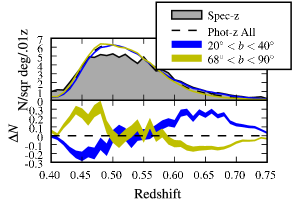
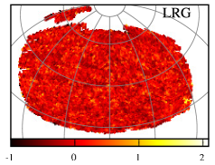
We base our study on the Sloan Digital Sky Survey (SDSS) (Adelman-McCarthy et al., 2008) Luminous Red Galaxy (LRG) sample. The photometric galaxy catalog traces large-scale structure to over 7500 square degrees of contiguous sky. LRGs are elliptical galaxies in massive galaxy clusters representing large dark-matter halos (Blake et al., 2008), and are thought to be physically similar objects across their redshift range (Eisenstein et al., 2001; Wake et al., 2006). This makes them excellent, albeit sparse, tracers of the cosmic matter distribution on scales Mpc. Our sample is designed to match the spectroscopic targets in the 2SLAQ LRG survey (Cannon et al., 2006). In particular, we apply the stringent and cuts. Within the DR6 imaging area about the North Galactic Pole, the catalog includes 746,962 objects; for our fiducial sample, though, we use the 400,000 closest to the median in redshift. Photometric redshifts are obtained from Oyaizu et al. (2008); we use the results from the CC2 algorithm. The median photometric error of the sample is . The redshift distribution is plotted in Fig. 1. It extends from with median . A map of the projected density is shown in Fig. 3.
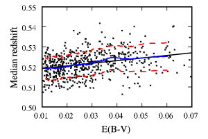
We find a systematic trend in the photometric redshift distribution with Galactic latitude; see Fig. 1. At low latitude, the distribution shifts toward higher redshift. Although the shift in the median redshift is smaller than the typical redshift error, it produces a strong gradient in the galaxy density at high and low redshift where the selection function is steep, which contaminates the 3D density reconstruction. We attribute this to residual errors in the Galactic extinction correction. The trend of median redshift with extinction, E(B-V), is shown in Fig. 2. Due to this issue, the useable redshift range is limited to the peak of the distribution, as we discuss in §4.3.
2.2. Microwave maps
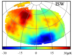
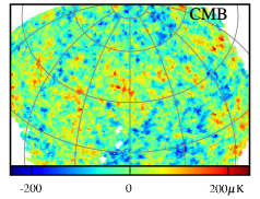
We use WMAP five-year maps, quoting results from the the Q, V and W frequency band maps, in which the individual differencing assembly maps have been co-added. To estimate Galactic foreground contamination, we use the foreground-reduced Q, V and W maps, the Markov-chain Monte Carlo (MCMC) derived temperature map and the Internal Linear Combination (ILC) map, all of which are described by Gold et al. (2009). The Q, V and W foreground reduced maps are full-resolution maps with best-fit foreground templates subtracted, preserving the noise properties of the original maps. The MCMC map was produced using a Monte Carlo joint fit of the CMB temperature, polarization and foregrounds. The map is smoothed at 1° full-width half-max resolution. The ILC map is foreground-cleaned using a minimum-variance fit of the foreground templates. It is smoothed to 1° resolution. We present the results from the ILC map even though its noise properties are not characterized. To each map we apply the KQ75 galactic foreground and point source mask. We carry out all analyses using the Healpix111http://healpix.jpl.nasa.gov pixelization scheme at a resolution of 55′/pixel () (Górski et al., 2005), at finer resolution than the ° scales where the linear ISW effect is thought to operate. The MCMC map is shown in Fig. 3.
3. ISW map construction
The ISW-induced temperature is an integral over the time-derivative of the gravitational potential . In terms of the conformal time , the temperature fluctuation along a line of sight, is (Sachs & Wolfe, 1967)
| (1) |
In linear theory, evolves with the growth factor as . In a flat, matter dominated universe , but in CDM, it deviates from this at low redshift due to accelerated expansion. We obtain the time derivative of the potential assuming linear theory, i.e.
| (2) |
We model the density field in the survey using a Voronoi tessellation (e.g. Okabe et al., 2000; van de Weygaert & Schaap, 2009). Each galaxy occupies a polyhedral Voronoi cell of points closer to that galaxy than to any other. The volume of that cell gives a natural estimate of the galaxy’s overdensity, , where is the average volume of a galaxy at redshift .
We compute the potential as a direct sum over these polyhedral cells of volume and overdensity , concentrated at the comoving positions of their galaxies. In the Newtonian limit, the potential is
| (3) | |||||
| (4) |
Here, is the critical density at . In evaluating this expression, we put the whole survey at the median redshift of the sample, , multiplying by a factor . After computing the potential, we then divide by this factor to get the proper amplitude. Explicitly, the observed density is the true density convolved with the photometric redshift error distribution, and attenuated by the top-hat survey window function: .
Our method is relatively slow computationally, since it involves a sum over all galaxies for each point where the potential is evaluated, and a Voronoi tessellation. For our fiducial galaxy sample, the computation takes a few hours using several CPU’s, while a fast fourier transform method could take less than a minute on one CPU. However, our method easily allows the true (curved) geometry of the LRG sample to be included, and integrated through to . Also, the contribution to the potential from each galaxy is included in a natural way using the parameter-free, highly adaptive Voronoi method.
We added a buffer of galaxies around the survey, and filled survey holes with galaxies sampled at the mean density at each redshift, as in Granett et al. (2008). Hole galaxies (comprising 1/300 of the galaxies) were included in the potential sum, but galaxies neighboring any buffer galaxy (i.e. affected by the edge) were not. To get the mean galaxy volume function , we spline-interpolated between galaxy volumes averaged in bins of logarithmic width .
To get the predicted ISW map, we integrated the signal (Eq. (1)) through lines of sight of Healpix pixels. We integrated from to 1.5 times the farthest distance of a galaxy in the survey, sampling the potential at 10 (a sufficient number, according to convergence tests) equally spaced points in each of three regions: in front of, within, and behind the sample. In spots, the nonzero potential behind and in front of the survey generated 50% of the signal. To lessen the noise from galaxies happening to lie too close to a point where the potential was evaluated, we softened the potential by setting the distance to a galaxy to maxMpc). The resulting map is shown in Fig. 3.
A constant multiplicative bias factor is thought to describe the ratio of the galaxy to matter overdensity adequately on the large scales of the linear ISW effect: . In the case of the LRG sample, () (Blake et al., 2008). We expect the true ISW fluctuations to be lower than our construction by a factor of : . This dependence on the bias allows for to be fit directly, independent of the power spectrum amplitude.
4. Statistical significance
4.1. Amplitude fit
To judge the reality of the reconstructed ISW signal, we measure its contribution to the microwave sky with a template fit approach. The observed microwave temperature is the sum of the primary CMB anisotropy, galactic and extragalactic foreground contributions and the ISW signal, . The ISW anisotropy arises from the structure sampled by LRG galaxies corrected for the galaxy bias. We add the predicted ISW template with a scaling parameter , to be fit:
| (5) |
Fixing the ISW and foreground anisotropies, the likelihood function, in terms of the pixel CMB covariance matrix, , is,
| , | (6) |
and maximizing this over gives,
| (7) |
The variance of this estimator is,
| (8) |
This approach can be extended naturally to multiple correlated datasets through a joint fit of many template maps. The estimator is non-linear in the the ISW template. Thus, shot noise, arising in the galaxy survey, leads to a biased estimate of the amplitude. Perturbing the ISW template by , leads to an underestimate of the amplitude. Given shot noise variance, , that scales with the number of galaxies, the expected amplitude takes the form,
| (9) |
In the case of the ISW effect, the covariance matrix is dominated by the primary CMB. We estimate the covariance matrix using the best-fit angular power spectrum from WMAP5 convolved with the pixel window function and instrument beam: , where is the pixel window function, and is the instrument beam. Pixel noise is added according to the noise properties of the map considered. In the case of the ILC map, pixel noise is neglected because it is not characterized.
A correction to the covariance must be added to address the fact that we estimate the mean of the distribution from the sample itself. The covariance is where is the mean pixel value within the survey: . Expanding, this becomes Although this correction is for the SDSS survey area, neglecting it leads to an overestimate in the significance of the ISW signal.
Finally, the computed covariance matrix is ill-conditioned, leading to an unstable inversion. This is generally the case for a map covering only a fraction of the sky. We find a usable pseudo-inverse by computing the singular value decomposition of the matrix and zeroing the noisiest modes. The eigenvalue limit was chosen such that a stable inversion was produced for all CMB maps we considered.
4.2. Results
The calculation is carried out over the intersection of the galaxy survey footprint and CMB foreground mask, in total 9298 pixels.
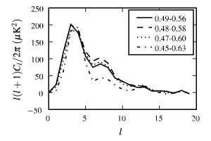
We tested ISW maps generated from four redshift cuts listed in Table 1 fit to the MCMC CMB map. The error was determined with Eq. (8). We find that the signal degrades in the wider redshift ranges in samples III and IV. The maximum signal was found in sample II, which includes of the galaxies about the median redshift, spanning . Including all galaxies reduces the significance by . We attribute this to contamination from a large-scale gradient in the galaxy density arising from a systematic shift in the redshift distribution discussed in §2.1. This error is not accounted for in our analysis and we limit ourselves to the sample II redshift range for our results. The differences between the ranges that we test are comparable to the size of the photometric redshift error, so adjusting the cut should not significantly bring in new structures affecting the intrinsic signal.
The power spectra of the ISW maps are shown in Fig. 4. The maps are multiplied by the best-fit value from Table 1. This normalization properly scales the spectra, aligning the peak at multipole . This scaling property with suggests that narrowing the redshift range acts as a smoothing kernel, washing out fluctuations in the potential. We further investigate this effect with simulations in §4.3.
We calculated the best-fit ISW amplitude for the Q, V and W maps, as well as for the various foreground reduced maps using sample II. The results are listed in Table 2, and are all consistent with a 2 signal.
There is little evidence for foreground contamination. Although there is a 0.2 difference between the V and W maps, the amplitudes found from the foreground-reduced maps agree with the raw co-added maps. This suggests that the slight color dependence is not due to foreground contamination, but may arise from other differences such as the map beams and noise properties. Furthermore, the ILC and MCMC maps agree with each other, and match the V filter. This finding is consistent with previous ISW studies, including Ho et al. (2008) who place an upper limit of 0.3 on the effect of foreground contamination on the ISW detection significance.
Li et al. (2009) found a large-scale correlation in WMAP data between the number of observation passes made over a region of sky and the derived temperature which could affect the ISW measurement. To check for this, we computed the template fit between the number of observations of each pixel and the temperature of the Q map at resolution. Over the SDSS area, we find no correlation on the mean pixel temperature with . It is still possible that there is an effect from the disparity in observation number between the plus and minus antennae as reported by Li et al. (2009) which will require further investigation.
4.3. Interpretation
The constructed potential is affected by the survey window function, photometric redshift errors and shot noise. We account for these effects with the aid of simulations. We generate mock LRG catalogs from Gaussian large-scale structure simulations extending to with 40-Mpc cells and model the SDSS LRG sample as a slab cut out from this volume. We used a fast fourier transform to compute the potential in this rectangular geometry, enabling the results of hundreds of simulations to be averaged together. The template fit in this case measures the contribution of the survey slab’s ISW signal to the full ISW signal integrated from to 2. We model redshift errors by convolving the density field with a Gaussian kernel with along the radial direction and introduce shot noise by sampling the field according to the survey selection function.
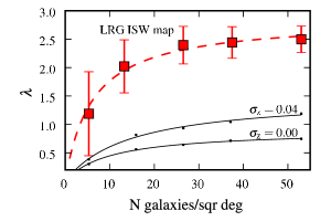
Fig. 5 shows the effect of shot noise in the simulations and on the LRG measurement. We under-sampled the LRG catalog to create ISW maps with increased shot noise and fit the trend with Eq. (9). Although the amplitude measured from LRGs is higher than from simulations, the trends are similar. Shot noise biases the measurement low; in Fig. 5, the asymptotic limit to from the LRGs is 2.8, to be compared with the measured result from the full map, 2.51, in Table 2.
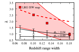
The redshift error convolution and survey window function act to bias high. This can be understood due to the smoothing effect redshift errors have on the reconstructed potential. Fig. 6 shows the results of the simulations using the four tested redshift cuts. The measured trend in with survey width does not agree with the simulation results, but we attribute the deviation in the wider redshift samples to the large-scale gradient in the galaxy density in the tail of the redshift distribution (discussed in §2.1), and so, we do not consider these points for the cosmological interpretation.
After modeling both shot noise and redshift error effects, we make a simple correction to our measurements by normalizing by the results measured from simulations. In sample II, is corrected by a factor of 1.2. The corrected values are listed in Tables 1 and 2. Our measurement is a factor of above the CDM simulation results, within the 1- range of cosmic variance. This result is in concordance with the higher-than-expected ISW amplitude found by Ho et al. (2008), Giannantonio et al. (2008) and others, and is consistent with our own correlation function measurements presented in §5.
| redshift | N | Amplitude | Amplitude | ||
|---|---|---|---|---|---|
| range | uncorrected | corrected | |||
| I | 0.49-0.56 | 300 | 2.2 | 1.9 | |
| II | 0.48-0.58 | 400 | 2.1 | 2.0 | |
| III | 0.47-0.60 | 500 | 1.7 | 1.9 | |
| IV | 0.45-0.63 | 600 | 1.0 | 1.4 |
| Amplitude | Amplitude | ||
|---|---|---|---|
| Map | uncorrected | corrected | |
| Q Coadd | 2.0 | 2.0 | |
| V Coadd | 2.1 | 2.1 | |
| W Coadd | 1.8 | 1.8 | |
| Q FG reduced | 1.9 | 2.0 | |
| V FG reduced | 2.1 | 2.1 | |
| W FG reduced | 1.8 | 1.9 | |
| MCMC | 2.1 | 2.0 | |
| ILC | 2.1 | 2.0 |
5. Cross-correlation amplitude
5.1. Galaxy - CMB temperature correlation
The standard measure of the ISW effect is the galaxy overdensity-CMB temperature cross-correlation. The measurement has been made on the SDSS LRG dataset at the level (Ho et al., 2008; Giannantonio et al., 2008).
The expected angular power spectrum in the flat-sky limit, see e.g. Afshordi et al. (2004), is an integral over the line-of-sight distance ,
| (10) | |||||
where, is the galaxy selection function normalized by , is the growth factor and is the matter power spectrum at redshift . The correlation function in real space is,
| (11) |
where are the Legendre polynomials.
We measure the goodness-of-fit against a fiducial model scaled to the data. A one parameter fit is sufficient because variations in cosmology affect the ISW amplitude, but have little effect on the shape of the spectrum (Padmanabhan et al., 2005). We apply the same template fit estimator (Eq. (7)) in the fashion of Ho et al. (2008): given an observed data vector, , and model template, , we find the best fit amplitude, , for the model . The maximum likelihood estimate of the scale amplitude is , with variance , where is the covariance matrix. In the case of the angular power spectrum, . Given a fixed cosmological model, the free scaling is a constraint on the product of the galaxy bias and normalization of the power spectrum, .
We use SpICE (Szapudi et al., 2001) to estimate the spectrum for multipoles , the limits of which are set by the resolution of the map and the extent of the survey. The measured angular power spectrum is binned into 15 logarithmic band powers.
We consider only CMB variance in the error analysis. Neglecting the cosmic variance in the galaxy field leads to an underestimate of the errors by 10% (Cabré et al., 2007). We estimate the covariance matrix in a Monte-Carlo procedure with 2000 realizations of the CMB generated according to the best fit WMAP5 angular power spectrum. We consider here the correlation with the MCMC CMB map, which we model using an instrumental beam with 1° full-width half-max.
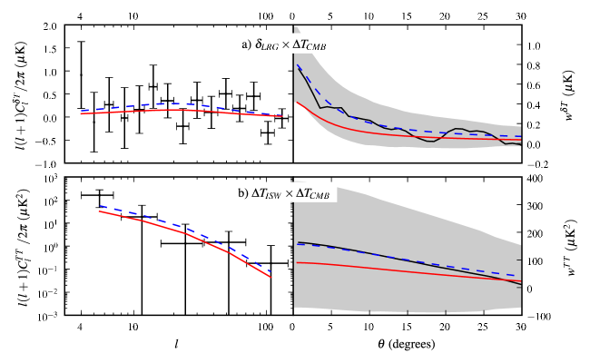
The cross-correlation results for the MCMC map are plotted in Fig. 7. The best fit amplitude is , a measurement. This is consistent with previous results using the LRG dataset(Ho et al., 2008; Giannantonio et al., 2008). We find that the signal is a factor of 1.9 greater than the CDM prediction with =2.2 and .
5.2. ISW-cleaned CMB map
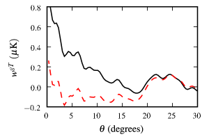
We now ask whether the constructed ISW map contains the signal found in the galaxy-CMB cross-correlation. We produce a cleaned CMB map by subtracting the constructed ISW template. The template is scaled by the best fit amplitude from Table 2. The cross-correlation of the cleaned CMB map with the LRG map is shown in Fig. 8. We find that the subtraction effectively nulls the correlation signal. This agreement strengthens the claim that the correlation is of the form expected from the ISW effect.
5.3. ISW - CMB temperature correlation
The ISW power spectrum gives a further measure with which to characterize our ISW construction. The cross-correlation between the reconstructed ISW map and the CMB temperature measures the ISW auto-power spectrum, and, by construction it is boosted by one power of the galaxy bias: . In the flat-sky limit the expected spectrum, e.g. Cooray (2002a), is,
| (12) | |||||
The ISW power is dominated by structures at low redshift which are not captured by our map. To account for this, we limit the integral in Eq. (12) from , the approximate redshift range of the survey. We carry out a fit to this model, again using Monte-Carlo realizations of the CMB to estimate the covariance. The measurement is plotted in Fig. 7. The best-fit amplitude is a factor of above CDM. Though the detection is marginal, it is consistent with the amplitudes measured above.
6. Supervoids and Superclusters
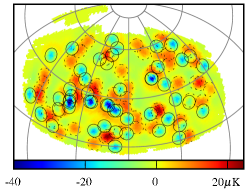
Recently we detected the imprints of voids and clusters on the CMB and attributed the finding to the linear ISW effect (Granett et al., 2008). The same SDSS LRG dataset at discussed here was used in that work, although with minor differences in the selection criteria and photometric redshifts. Thus, with the ISW signal reconstruction, we can further investigate the result and place limits on the role of linear ISW in the measurement. We also reassess the significance of the measurement with a template fit on the CMB.
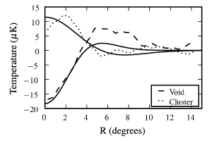
The 50 voids and 50 clusters presented by Granett et al. (2008) are strongly correlated with the CMB. The clusters, on average, fall on hot spots on the CMB, while the voids are cold. The mean temperature profiles on the CMB are plotted in Fig. 9. We re-examine the significance of the correlation with the template-fitting analysis used above, using a template constructed with the mean profiles of the voids and clusters. A compensated model was chosen to fit the profiles to ensure that the mean of the map is zero. For simplicity we use a “Mexican hat” Laplacian of a Gaussian for the functional, fitting for the amplitude and width. The template fit confirms the significance of the measurement found previously: we find . This high signal is not surprising because the void and cluster profiles were measured on the CMB, although it does confirm the peculiarity of these sites on the CMB.
If this correlation is due to the linear ISW effect, we would expect the signal to be contained in the constructed ISW map presented here. However, we find that the mean temperature of the clusters and voids on the ISW map is not significant. The temperature difference between clusters and voids is , and stacking the clusters and voids separately does give weak hot and cold spots. We measure the temperature in a 4° compensated aperture. The error bar was measured through a Monte-Carlo procedure using random locations within the survey. This result contradicts the suggestion that the signal is due to the linear ISW effect.
7. Conclusions
We implement a template fit measurement of the ISW signature imprinted on the CMB from structures traced by SDSS luminous red galaxies at with photometric redshifts. The approach uses the density information in the galaxy survey to remove the effects of local cosmic variance from the ISW measurement. The detection significance is 2, which is consistent with the cross-correlation statistic.
Our measured amplitude confirms the cross-correlation finding, that the signal is 1 higher than the CDM prediction. The evidence suggests that this amplitude arises from variance on the CMB (Ho et al., 2008), or alternative ISW physics, although we cannot exclude cosmic variance in the galaxy sample.
In principle, the template fit simplifies the error analysis and cosmological interpretation, because a Monte-Carlo procedure is not required to assess the role of cosmic variance in the galaxy sample, and multiple datasets can be combined naturally. On the other hand, the measurement is influenced by a number of systematic effects that do hinder the way towards precision cosmology. First, contamination by foreground emission must be subtracted from the CMB and the accuracy of the subtraction ultimately limits the ISW detection. This is also true of cross-correlation function studies. Second, shot noise in the galaxy survey biases the estimator, but in a largely correctable fashion. In the case of the LRG survey, we estimate that the effect is . Third, the photometric redshift errors severely degrade the reconstructed density and potential 3D maps, leading to a biased estimate of the template amplitude. In simulations of the LRG catalog, the template signal was reduced by a factor of 2. We expect that this bias can be mitigated by using cosmological density reconstruction techniques that take the redshift errors as a Bayesian prior (e.g. Enßlin et al., 2008), and the effect can be corrected with simulations.
The ISW template fit provides a unique constraint on cosmological parameters. In particular, because the ISW reconstruction is made from a biased tracer, the template fit constrains the galaxy bias independently of the the power spectrum amplitude, . Precision results from the ISW signal will become feasible with new all-sky survey projects, such as Pan-STARRS (Kaiser, 2004).
In this context, we further investigated our measurement of imprints of Mpc supervoids and superclusters on the CMB (Granett et al., 2008). We confirm that the signal is present in WMAP data at confidence with a template fit. However, we find that the signal has much lower amplitude in the linear ISW map constructed from LRGs than in the WMAP data.
References
- Adelman-McCarthy et al. (2008) Adelman-McCarthy, J. K. et al. 2008, ApJS, 175, 297, arXiv:0707.3413
- Afshordi et al. (2004) Afshordi, N., Loh, Y.-S., & Strauss, M. A. 2004, Phys. Rev. D, 69, 083524, astro-ph/0308260
- Barreiro et al. (2008) Barreiro, R. B., Vielva, P., Hernandez-Monteagudo, C., & Martinez-Gonzalez, E. 2008, IEEE Journal of Selected Topics in Signal Processing, vol. 2, issue 5, pp. 747-754, 2, 747, 0809.2557
- Blake et al. (2008) Blake, C., Collister, A., & Lahav, O. 2008, MNRAS, 385, 1257, arXiv:0704.3377
- Boughn & Crittenden (2004) Boughn, S., & Crittenden, R. 2004, Nature, 427, 45, astro-ph/0305001
- Cabré et al. (2007) Cabré, A., Fosalba, P., Gaztañaga, E., & Manera, M. 2007, MNRAS, 381, 1347, astro-ph/0701393
- Cabré et al. (2006) Cabré, A., Gaztañaga, E., Manera, M., Fosalba, P., & Castander, F. 2006, MNRAS, 372, L23, astro-ph/0603690
- Cai et al. (2009) Cai, Y.-C., Cole, S., Jenkins, A., & Frenk, C. 2009, MNRAS, 648, 0809.4488
- Cannon et al. (2006) Cannon, R. et al. 2006, MNRAS, 372, 425, astro-ph/0607631
- Cooray (2002a) Cooray, A. 2002a, Phys. Rev. D, 65, 103510, astro-ph/0112408
- Cooray (2002b) ——. 2002b, Phys. Rev. D, 65, 083518, astro-ph/0109162
- Corasaniti et al. (2005) Corasaniti, P.-S., Giannantonio, T., & Melchiorri, A. 2005, Phys. Rev. D, 71, 123521, astro-ph/0504115
- Crittenden & Turok (1996) Crittenden, R. G., & Turok, N. 1996, Phys. Rev. Lett., 76, 575, astro-ph/9510072
- de Oliveira-Costa et al. (1999) de Oliveira-Costa, A., Tegmark, M., Gutierrez, C. M., Jones, A. W., Davies, R. D., Lasenby, A. N., Rebolo, R., & Watson, R. A. 1999, ApJ, 527, L9, astro-ph/9904296
- Dent et al. (2009) Dent, J. B., Dutta, S., & Weiler, T. J. 2009, Phys. Rev. D, 79, 023502, 0806.3760
- Eisenstein et al. (2001) Eisenstein, D. J. et al. 2001, AJ, 122, 2267, astro-ph/0108153
- Enßlin et al. (2008) Enßlin, T. A., Frommert, M., & Kitaura, F. S. 2008, ArXiv e-prints, 0806.3474
- Fosalba & Gaztañaga (2004) Fosalba, P., & Gaztañaga, E. 2004, MNRAS, 350, L37, astro-ph/0305468
- Fosalba et al. (2003) Fosalba, P., Gaztañaga, E., & Castander, F. J. 2003, ApJ, 597, L89, astro-ph/0307249
- Frommert et al. (2008) Frommert, M., Enßlin, T. A., & Kitaura, F. S. 2008, MNRAS, 391, 1315, 0807.0464
- Giannantonio & Crittenden (2007) Giannantonio, T., & Crittenden, R. 2007, MNRAS, 381, 819, 0706.0274
- Giannantonio et al. (2006) Giannantonio, T. et al. 2006, Phys. Rev. D, 74, 063520, astro-ph/0607572
- Giannantonio et al. (2008) Giannantonio, T., Scranton, R., Crittenden, R. G., Nichol, R. C., Boughn, S. P., Myers, A. D., & Richards, G. T. 2008, Phys. Rev. D, 77, 123520, 0801.4380
- Gold et al. (2009) Gold, B. et al. 2009, ApJS, 180, 265, 0803.0715
- Górski et al. (2005) Górski, K. M., Hivon, E., Banday, A. J., Wandelt, B. D., Hansen, F. K., Reinecke, M., & Bartelmann, M. 2005, ApJ, 622, 759, astro-ph/0409513
- Granett et al. (2008) Granett, B. R., Neyrinck, M. C., & Szapudi, I. 2008, ApJ, 683, L99, arXiv:0805.3695
- Hansen et al. (2005) Hansen, F. K., Branchini, E., Mazzotta, P., Cabella, P., & Dolag, K. 2005, MNRAS, 361, 753, astro-ph/0502227
- Hernández-Monteagudo (2008) Hernández-Monteagudo, C. 2008, A&A, 490, 15, arXiv:0805.3710
- Ho et al. (2008) Ho, S., Hirata, C., Padmanabhan, N., Seljak, U., & Bahcall, N. 2008, Phys. Rev. D, 78, 043519, arXiv:0801.0642
- Hunt & Sarkar (2008) Hunt, P., & Sarkar, S. 2008, ArXiv e-prints, arXiv:0807.4508
- Inoue & Silk (2007) Inoue, K. T., & Silk, J. 2007, ApJ, 664, 650, astro-ph/0612347
- Kaiser (2004) Kaiser, N. 2004, in Society of Photo-Optical Instrumentation Engineers (SPIE) Conference Series, Vol. 5489, Society of Photo-Optical Instrumentation Engineers (SPIE) Conference Series, ed. J. M. Oschmann, Jr., 11–22
- Komatsu et al. (2009) Komatsu, E. et al. 2009, ApJS, 180, 330, arXiv:0803.0547
- Li et al. (2009) Li, T.-P., Liu, H., Song, L.-M., Xiong, S.-L., & Nie, J.-Y. 2009, ArXiv e-prints, 0905.0075
- Loverde et al. (2007) Loverde, M., Hui, L., & Gaztañaga, E. 2007, Phys. Rev. D, 75, 043519, arXiv:astro-ph/0611539
- Maturi et al. (2007) Maturi, M., Dolag, K., Waelkens, A., Springel, V., & Enßlin, T. 2007, A&A, 476, 83, arXiv:0708.1881
- McEwen et al. (2007) McEwen, J. D., Vielva, P., Hobson, M. P., Martínez-González, E., & Lasenby, A. N. 2007, MNRAS, 376, 1211, astro-ph/0602398
- McEwen et al. (2008) McEwen, J. D., Wiaux, Y., Hobson, M. P., Vandergheynst, P., & Lasenby, A. N. 2008, MNRAS, 384, 1289, arXiv:0704.0626
- Nolta et al. (2004) Nolta, M. R. et al. 2004, ApJ, 608, 10, astro-ph/0305097
- Okabe et al. (2000) Okabe, A., Sugikara, K., & Chia, S. N. 2000, Spatial Tessellations, 2nd edn. (New York: Wiley)
- Oyaizu et al. (2008) Oyaizu, H., Lima, M., Cunha, C. E., Lin, H., Frieman, J., & Sheldon, E. S. 2008, ApJ, 674, 768, arXiv:0708.0030
- Padmanabhan et al. (2005) Padmanabhan, N., Hirata, C. M., Seljak, U., Schlegel, D. J., Brinkmann, J., & Schneider, D. P. 2005, Phys. Rev. D, 72, 043525, astro-ph/0410360
- Pietrobon et al. (2006) Pietrobon, D., Balbi, A., & Marinucci, D. 2006, Phys. Rev. D, 74, 043524, astro-ph/0606475
- Pogosian et al. (2005) Pogosian, L., Corasaniti, P. S., Stephan-Otto, C., Crittenden, R., & Nichol, R. 2005, Phys. Rev. D, 72, 103519, astro-ph/0506396
- Raccanelli et al. (2008) Raccanelli, A., Bonaldi, A., Negrello, M., Matarrese, S., Tormen, G., & de Zotti, G. 2008, MNRAS, 386, 2161, arXiv:0802.0084
- Rassat et al. (2007) Rassat, A., Land, K., Lahav, O., & Abdalla, F. B. 2007, MNRAS, 377, 1085
- Rees & Sciama (1968) Rees, M. J., & Sciama, D. W. 1968, Nature, 217, 511
- Rudnick et al. (2007) Rudnick, L., Brown, S., & Williams, L. R. 2007, ApJ, 671, 40, arXiv:0704.0908
- Sachs & Wolfe (1967) Sachs, R. K., & Wolfe, A. M. 1967, ApJ, 147, 73
- Sakai & Inoue (2008) Sakai, N., & Inoue, K. T. 2008, Phys. Rev. D, 78, 063510, arXiv:0805.3446
- Schlegel et al. (1998) Schlegel, D. J., Finkbeiner, D. P., & Davis, M. 1998, ApJ, 500, 525, arXiv:astro-ph/9710327
- Scranton et al. (2003) Scranton, R. et al. 2003, ArXiv Astrophysics e-prints, astro-ph/0307335
- Sunyaev & Zeldovich (1972) Sunyaev, R. A., & Zeldovich, Y. B. 1972, Comments on Astrophysics and Space Physics, 4, 173
- Szapudi et al. (2001) Szapudi, I., Prunet, S., & Colombi, S. 2001, ApJ, 561, L11
- van de Weygaert & Schaap (2009) van de Weygaert, R., & Schaap, W. 2009, in Data Analysis in Cosmology, ed. V. Martinez, E. Saar, E. Martínez-Gonzáles, & M.-J. Pons-Bordería (Berlin: Springer), arXiv:0708.1441
- Wake et al. (2006) Wake, D. A. et al. 2006, MNRAS, 372, 537, astro-ph/0607629