Self-organization in nonadditive systems with external noise

Abstract

A nonadditive generalization of Klimontovich’s S-theorem [G. B. Bağcı, Int.J. Mod. Phys. B 22, 3381 (2008)] has recently been obtained by employing Tsallis entropy. This general version allows one to study physical systems whose stationary distributions are of the inverse power law in contrast to the original S-theorem, which only allows exponential stationary distributions. The nonadditive S-theorem has been applied to the modified Van der Pol oscillator with inverse power law stationary distribution. By using nonadditive S-theorem, it is shown that the entropy decreases as the system is driven out of equilibrium, indicating self-organization in the system. The allowed values of the nonadditivity index $q$ are found to be confined to the regime $(0.5,1.0]$.

I
Introduction

Klimontovich [1] originally proposed S-theorem (Self-organization theorem) in order to generalize Gibbs’ theorem [2] to open systems, since the latter rests on the assumption that all the compared distributions have the same mean energy values. However, this assumption does not hold when one studies open systems with energy or matter influx. Therefore, Klimontovich considered equating the mean energies of different states before comparing the associated entropies. This process of equating mean energies of different states is called renormalization (not to be confused by renormalization in quantum field theory) by Klimontovich. However, S-theorem did not only succeed in generalizing Gibbs’ theorem but gained recognition as a criterion of self-organization in open systems, since it allows us compare even the stationary nonequilibrium distributions [3-7].

In open systems, we have some control parameters, which determine the stationary distributions of the system. As the control parameter increases, the system recedes away from equilibrium, increasing its mean energy and entropy. S-theorem orders the associated entropies in such a way that the state closer to equilibrium possesses a greater entropy compared to the other states. In other words, we have a more ordered state as the control parameter increases. This decrease of entropy on ordering is called self-organization by Haken [8].

It is worth noting that the use of S-theorem is not limited to analytical models. It has also been used for many numerical models such as logistic map [9], heart rate variability [10, 11] and the analysis of electroencephalograms of epilepsy patients [12] as a criterion of self-organization.

Despite all its past successes, S-theorem rests on the use of Boltzmann-Gibbs (BG) entropy. Therefore, it is devised to handle cases with exponential stationary distributions. On the other hand, the study of open systems often results in stationary distributions of the inverse power law form. Hence, it is important to generalize S-theorem so that its use can be extended to open systems with stationary distributions of inverse power law form. Such a generalization has recently been made [13] by the employment of Tsallis entropy [14-16] instead of BG entropy. However, in Ref. [13], a rigorous application of the nonadditive S-theorem was not present [17]. We here present an application of the generalized S-theorem to the modified Van der Pol oscillator with inverse power law stationary distributions.

The paper is organized as follows: In Section II, we review the nonadditive S-theorem for open nonadditive systems. The application of the nonadditive S-theorem to the modified Van der Pol oscillator is presented in Section III. Concluding remarks will be presented in Section IV.

II The nonadditive S-theorem

We begin by supposing that we have two distinct probability distributions, i.e., $r_{eq}$ and $p$, corresponding to equilibrium and nonequilibrium states, respectively. In open systems, the stationary equilibrium distribution is defined as the distribution corresponding to the state where the relevant control parameter is set to zero. Similarly, any other stationary state with non-zero control parameter is defined as the nonequilibrium state. As the value of control parameter increases, the system recedes away from equilibrium state. The nonadditive S-theorem is equivalent to showing that the renormalized entropy defined as

$$R_{q}[p\|{\widetilde{r}_{eq}}]\equiv\ S_{q}^{neq}(p)-\widetilde{S}_{q}^{eq}(\widetilde{r}_{eq})$$ (1)

is negative i.e., $R_{q}<0$, since this implies that $\widetilde{S}_{q}^{eq}>S_{q}^{neq}$. $S_{q}$ denotes nonadditive Tsallis entropy

$$S_{q}(p)=\frac{\sum_{i}^{W}p_{i}^{q}-1}{1-q},$$ (2)

where $p_{\text{i }}$ is the probability of the system in the $i$th microstate, $W$ is the total number of the configurations of the system. The entropic index $q$ is called the nonadditivity parameter. As $q\rightarrow 1$, the nonadditive Tsallis entropy becomes

$$S_{q\rightarrow 1}=-\sum_{i=1}^{W}p_{i}\ln p_{i},$$ (3)

which is the usual BG entropy.

We denote the equilibrium distribution and the associated entropy in Eq. (1) by a tilde, since this is not the original equilibrium entropy but the one obtained after the effective mean energy equalization i.e., renormalization. This equalization is necessary, because the mean energies of equilibrium and nonequilibrium states are different. We define effective mean energy $U_{\text{eff}}$ in terms of the equilibrium state as

$$U_{\text{eff}}=\ln_{q}\left(\frac{1}{r_{eq}}\right)\;,$$ (4)

where the $q$-logarithm function $\ln_{q}(x)$ is defined as

$$\ln_{q}(x)=\frac{x^{1-q}-1}{1-q}.$$ (5)

The definition of effective mean energy in Eq. (4) is central to our generalization and therefore requires some explanation. The effective mean energy is defined in terms of the equilibrium distribution obtained from the maximization of Tsallis entropy subject to ordinary constraints. Therefore, the application of the effective mean energy definition in Eq. (4) to the equilibrium distribution $r_{eq}=[1-(q-1)\beta\varepsilon_{i}]^{1/(q-1)}$ (apart from normalization) results in $U_{\text{eff}}=\beta\varepsilon_{i}$. This explains why it is called effective mean energy since it is proportional to the multiplication of the Lagrange multiplier $\beta$ associated with the internal energy constraint and the energy of the $i$th microstate. We can write the equalization of the effective mean energies of two states as

$$\left\langle U_{\text{eff}}\right\rangle^{(req)}=\left\langle U_{\text{eff}}\right\rangle^{(neq)},$$ (6)

where superscripts $(req)$ and $(neq)$ denote the renormalized equilibrium and ordinary nonequilibrium states, respectively. From now on, we will drop the subscript $(eq)$ from the equilibrium probability distribution $r$. Therefore, it should be understood that the probability distributions $r$ and $\widetilde{r}$ denote the ordinary and renormalized equilibrium distributions, respectively. Using normalization and the effective mean energy definition defined in Eq. (4), Eq. (6) can be written in a more explicit form as

$$\sum_{i}r_{i}^{q-1}\widetilde{r}_{i}=\sum_{i}r_{i}^{q-1}p_{i},$$ (7)

where $\widetilde{r}$ is the renormalized equilibrium distribution obtained after equating the mean energies.

We then substitute Tsallis entropy given by Eq. (2) into Eq. (1) to obtain an explicit nonadditive renormalized entropy expression

$$R_{q}[p\|\widetilde{r}]=-\left[\frac{1}{(q-1)}\left(\sum_{i}p_{i}^{q}-\sum_{i}\widetilde{r}_{i}^{q}\right)\right].$$ (8)

We can rewrite the above equation as

$$R_{q}[p\|\widetilde{r}]=-\left[\frac{1}{(q-1)}\left(\sum_{i}p_{i}^{q}-\sum_{i}\widetilde{r}_{i}^{q}+(q-1)\sum_{i}\widetilde{r}_{i}^{q}-(q-1)\sum_{i}\widetilde{r}_{i}^{q}\right)\right].$$ (9)

We then substitute $\widetilde{r}_{i}=r_{i}/C$ into Eq. (7) in order to calculate $\sum_{i}\widetilde{r}_{i}^{q}$ explicitly where $C$ is normalization constant. This yields

$$\sum_{i}\widetilde{r}_{i}^{q}=\sum_{i}p_{i}\widetilde{r}_{i}^{q-1}.$$ (10)

The substitution of the relation in Eq. (10) into Eq. (9) finally results

$$R_{q}[p\|\widetilde{r}]=-\left(\frac{\sum_{i}p_{i}^{q}}{q-1}+\sum_{i}\widetilde{r}_{i}^{q}-\frac{1}{q-1}\sum_{i}p_{i}\widetilde{r}_{i}^{q-1}-\sum_{i}p_{i}\widetilde{r}_{i}^{q-1}\right).$$ (11)

In order to consider Eq. (11) as the nonadditive S-theorem, we must show that the nonadditive renormalized entropy $R_{q}(p\|\widetilde{r})$ is always negative. This can be deduced from the fact that the expression within the parentheses is the nonadditive relative entropy $K_{q}[p\|\widetilde{r}]$ [18] i.e.,

$$K_{q}[p\|\widetilde{r}]=\frac{\sum_{i}p_{i}^{q}}{q-1}+\sum_{i}\widetilde{r}_{i}^{q}-\frac{1}{q-1}\sum_{i}p_{i}\widetilde{r}_{i}^{q-1}-\sum_{i}p_{i}\widetilde{r}_{i}^{q-1}.$$ (12)

Since the nonadditive relative entropy $K_{q}[p\|\widetilde{r}]$ is positive for all positive $q$ values, we conclude that

$$R_{q}[p\|\widetilde{r}]=S_{q}(p)-\widetilde{S}_{q}(\widetilde{r})=-K_{q}[p\|\widetilde{r}]<0.$$ (13)

It is worth noting that the main reason for excluding negative $q$ values from the above discussion is thermodynamic stability of Tsallis entropy, since it is stable only for positive values of $q$ [19].

The nonadditive generalization of S-theorem requires the use of ordinary probability distributions i.e., first choice of constraints in nonadditive thermostatistics, instead of escort distributions i.e., third choice in nonadditive thermostatistics. In fact, even the nonadditive relative entropy expression we have used is the one compatible with the ordinary probability distribution [13, 18].

It should be noted that the ordinary S-theorem by Klimontovich is recovered in the $q\rightarrow 1$ limit. This can be seen from the inspection of Eq. (13), since Tsallis entropy expressions become BG entropies, whereas all the stationary distributions become exponential in the $q\rightarrow 1$ limit. The nonadditive relative entropy in Eq. (13) becomes Kullback-Leibler relative entropy in the aforementioned limit i.e., $K[p\|r]\equiv\sum_{i}p_{i}\ln(p_{i}/r_{i})$ [20], which is positive definite, ensuring the negativity of the ordinary renormalized entropy.

III Noise-driven modified Van der Pol oscillator

In this section, we will study the noise-driven modified Van der Pol oscillator, which is classified by the following Ito-Langevin type two dimensional stochastic equation [21]

$$\dot{x} = \frac{\partial H}{\partial y}+\alpha^{2}f(H;u)\frac{\partial H}{\partial x}+\alpha\sigma g(H;u)\xi_{1}(t),$$

$$\dot{y} = -\frac{\partial H}{\partial x}+\beta^{2}f(H;u)\frac{\partial H}{\partial y}+\beta\sigma g(H;u)\xi_{2}(t).$$ (14)

These type of equations have been first formulated by Enz [22] in the framework of mixed-canonical-dissipative dynamics and later used to study nonlinear dynamical systems with noise [23, 24]. The term $H(x,y)$ denotes Hamiltonian. We will particularly consider the Hamiltonian of the form $H=\frac{1}{2}(x^{2}+y^{2})$, where $x$ and $y$ are fluctuating parameters. $f(H;u)$ and $g(H;u)$ are some arbitrary functions, which may depend on $H$ and some nonfluctuating control parameters $u=\{u_{1},u_{2}\}$. Gaussian white noise with intensity $\sigma=\sqrt{2D}$ is generated through $\xi_{i}$’s, where $\alpha$ and $\beta$ are real parameters. From now on, we will assume $\alpha=0$, $\beta=1$, and $g(H;u)=1$. Then, the most general stationary solution for the modified Van der Pol oscillator in Eq. (14) is given by

$$f_{0}(H)=C\exp\left[\frac{2}{\sigma^{2}}\int dHf(H,u_{1},u_{2})\right],$$ (15)

where $C$ is normalization constant.

As we remarked above, the function $f(H,u_{1},u_{2})$ is quite arbitrary and can be changed to another expression as long as the new expression can be written in terms of the energy $H$ and the control parameters. We choose the function $f(H,u_{1},u_{2})$ as

$$f(H,u_{1},u_{2})=\frac{-u_{1}-2u_{2}H}{1+\frac{(1-q)}{D}(u_{1}H+u_{2}H^{2})}$$ (16)

and the control parameters as $u_{1}=a=\gamma-a_{f}$ and $u_{2}=b/2$, where $\gamma$ is the linear friction coefficient, and $a_{f}$ is the feedback or control parameter. The term $b$ denotes the nonlinear friction coefficient. The corresponding stationary distribution, due to Eq. (15), takes the form

$$f_{0,q}(E)=C\exp_{2-q}\left(-\frac{aE+\frac{1}{2}bE^{2}}{D}\right)\;,$$ (17)

where $q$-exponential is defined by

$$\exp_{q}(x)=[1+(1-q)x]^{\frac{1}{1-q}}.$$ (18)

The stationary distribution in Eq. (17) is a $q$-exponential of the order $(2-q)$, not $q$. In order to understand this expression, it is important to remember that the nonadditive S-theorem requires the use of ordinary constraint. The stationary distribution compatible with the first constraint in nonadditive thermostatistics is given by $f_{0,q}(E)\propto\exp_{(2-q)}(-x)$. Following Klimontovich, we assume $b\left\langle E\right\rangle/\gamma\sim Db/\gamma^{2}\ll 1$ [4, 13], so that the corresponding equilibrium distribution associated with zero value of the control parameter is

$$r_{q}(E)=\frac{\gamma q}{D}\exp_{2-q}\left(-\frac{\gamma E}{D}\right)\;,$$ (19)

where $\gamma q/D$ is the normalization constant for $q$ values between 0 and 1. Next, we increase the control parameter to a value different from zero and create nonequilibrium state in the system. We set the feedback parameter $a_{f}$ equal to $\gamma$ so that the term $a$ becomes equal to 0. The distribution function can then be written as

$$p_{q}(E)=\sqrt{\frac{2(1-q)b}{D}}\left[B\left(\frac{1}{2},\frac{1}{1-q}-\frac{1}{2}\right)\right]^{-1}\left[1+(1-q)\frac{b}{2D}E^{2}\right]^{\frac{1}{q-1}}$$ (20)

for $0\leq q\leq 1$, where the normalization constant is inserted [25]. The renormalization of energies i.e., Eq. (7) becomes

$$\int_{0}^{\infty}dEE\widetilde{r}_{q}(E)=\int_{0}^{\infty}dEEp_{q}(E).$$ (21)

The integral on the right hand side can be easily solved and it yields

$$\int_{0}^{\infty}dEEp_{q}(E)=\sqrt{(1-q)}\left[B\left(\frac{1}{2},\frac{1}{1-q}-\frac{1}{2}\right)\right]^{-1}\sqrt{\frac{2D}{bq^{2}}}$$ (22)

for $0<q\leq 1$. On the other hand, the integral on the left is calculated as

$$\int_{0}^{\infty}dEE\widetilde{r}_{q}(E)=\frac{\widetilde{D}}{(2q-1)\gamma}$$ (23)

for $\frac{1}{2}<q\leq 1$. Therefore, Eq. (21), explicitly written, becomes

$$\widetilde{D}=(2q-1)\gamma\sqrt{(1-q)}\left[B\left(\frac{1}{2},\frac{1}{1-q}-\frac{1}{2}\right)\right]^{-1}\sqrt{\frac{2D}{bq^{2}}}$$ (24)

for $\frac{1}{2}<q\leq 1$. Therefore, the nonadditive renormalized entropy is calculated as

$$R_{q}[p\|\widetilde{r}]=(1-q)^{-1}\left[\frac{2(1-q)b}{D}\right]^{(q-1)/2}\left[B\left(\frac{1}{2},\frac{1}{1-q}-\frac{1}{2}\right)\right]^{-q}B\left(\frac{1}{2},\frac{q}{1-q}-\frac{1}{2}\right)-(1-q)^{-1}q^{q}\gamma^{q-1}\frac{\widetilde{D}^{1-q}}{(2q-1)}$$ (25)

for $\frac{1}{2}<q\leq 1$, where the renormalized noise intensity $\widetilde{D}$ is given by Eq. (24). The nonadditive renormalized entropy expression above is always negative for positive values of the nonadditivity parameter $q$ i.e., $R_{q}[p\|\widetilde{r}]<0$, since it is the negative of the nonadditive relative entropy $K_{q}[p\|\widetilde{r}]$ together with the renormalization of the corresponding mean energies. The nonadditive renormalized entropy in Eq. (25) is plotted in Figs. 1 and 2 for some particular values of the intensity of the random source $D$ and nonlinear friction coefficient $b$. However, it is important to understand that our results are independent of the random source intensity and nonlinear friction coefficient. The nonadditive renormalized entropy attains the value $-0.05$ in the $q\rightarrow 1$ limit. This is the exact value one would obtain if one would use Klimontovich’s additive renormalized entropy as a criterion of self-organization.

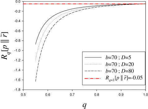
Figure 1: The plot of nonadditive renormalized entropy $R_{q}[p\|\widetilde{r}]$ versus the nonadditivity parameter $q$ for three representative values of random source intensity $D$, where nonlinear friction coefficient is $b$=70.

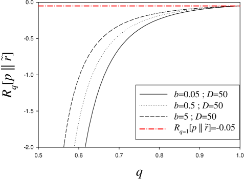
Figure 2: The plot of nonadditive renormalized entropy $R_{q}[p\|\widetilde{r}]$ versus the nonadditivity parameter $q$ for three representative values of nonlinear friction coefficient $b$, where random source intensity $D$=50.

IV Conclusions

Klimontovich’s original S-theorem is based on turning the ordinary reference distribution into the corresponding escort distribution where the exponent of the escort distribution is fixed through mean energy renormalization [3]. However, due to the use of BG entropy, original S-theorem is limited to the additive open systems, and exponential stationary distributions. In contrast, the nonadditive S-theorem is obtained only by using ordinary probability distributions. When we adopt nonadditive Tsallis entropy, we are required to use ordinary probability instead of escort distribution, since the nonadditivity index $q$ plays the role of the escort distribution’s exponent [13].

Klimontovich applied his original S-theorem to Van der Pol oscillator with exponential stationary distributions [26]. In this work, the nonadditive S-theorem has been applied to a modified Van der Pol oscillator with stationary distributions of inverse power law. It is interesting to note that we have modified Van der Pol model of Klimontovich only by changing the dissipative term $f(H,u_{1},u_{2})$. We have shown that the self-organization takes place as the control parameter increases from zero value, where the signature of the self-organization in this framework is the negativity of the nonadditive renormalized entropy. The nonadditive renormalized entropy attains the value $-0.05$ in the $q\rightarrow 1$ limit. This is exactly the same value one would obtain by using Klimontovich’s original S-theorem [4, 13].

The most important difference in changing the underlying dynamics so that the stationary distribution is of the q-exponential form is the confinement of the $q$ values to a range between 0.5 and 1. If one uses nonadditive renormalized entropy together with the exponential stationary distributions obtained from Klimontovich’s Van der Pol model, the nonadditivity index $q$ can take any value without limitations [13]. However, the change in the dynamics so as to make the stationary distributions of the Van der Pol model of q-exponential form, results in a spectrum of some privileged $q$ values. This seems to be a general feature one encounters whenever one studies physical systems depending on a control parameter [27, 28]. It is also worth remarking how the probability distribution of the first constraint in nonadditive thermostatistics i.e., $q$-exponential with order $(2-q)$, emerges in the numerical studies concerning systems depending upon control parameters [27, 28].

V ACKNOWLEDGEMENTS

We thank B. Bakar for his helpful comments. This work has been supported by TUBITAK (Turkish Agency) under the Research Project number 108T013.

References

- (1) Yu. L. Klimontovich, Z. Phys. B 66, 125 (1987).
- (2) J. W. Gibbs, Elementary Principles in Statistical Mechanics, Ox Bow Press, New York, 1992.
- (3) Yu. L. Klimontovich, Chaos, Solitons and Fractals 5, 1985 (1994).
- (4) Yu. L. Klimontovich, Physica A 142, 390 (1987).
- (5) Yu. L. Klimontovich, Turbulent Motion and the Structure of Chaos: A New Approach to the Statistical Theory of Open System, Kluwer Academic Publishers, Dordrecht, 1991.
- (6) Yu. L. Klimontovich, Physica Scripta 58, 549 (1998).
- (7) Yu. L. Klimontovich and M. Bonitz, Z. Phys. B 70, 241 (1988).
- (8) H. Haken, Information and Self-organization: A Macroscopic Approach to Complex Systems, Springer Verlag, Berlin, 2000.
- (9) P. Saparin, A. Witt, J. Kurths, V. Anischenko, Chaos, Solitons and Fractals4, 1907 (1994).
- (10) J. Kurths et al., Chaos 5, 88 (1995).
- (11) A. Voss et al., Cardiovasc. Res. 31, 419 (1996).
- (12) K. Kopitzki, P. C. Warnke, J. Timmer, Phys. Rev. E 58, 4859 (1998).
- (13) G. B. Bağcı, Int.J. Mod. Phys. B 22, 3381 (2008).
- (14) C. Tsallis, J.Stat. Phys. 52, 479 (1988).
- (15) E.M.F. Curado and C. Tsallis, J. Phys. A 24 (1991) L69; Corrigenda: J. Phys. A 24 (1991) 3187; 25, 1019 (1992).
- (16) C. Tsallis, R. S. Mendes, and A. R. Plastino, Physica A 261, 534 (1998).
- (17) In Ref. [13], the nonadditive S-theorem has been applied to the Van der Pol oscillator model of Klimontovich. However, the stationary distributions in that model were of exponential form. Therefore, although important for illustrative reasons, it cannot be considered as a rigorous application of the nonadditive S-theorem, since the nonadditive S-theorem relies on the use of Tsallis entropy, which requires the use of inverse power law stationary distributions.
- (18) S. Abe, G. B. Bağcı, Phys. Rev. E 71, 016139 (2005).
- (19) S. Abe, Phys. Rev. E 66, 046134 (2002).
- (20) R. Gray, Entropy and Information Entropy, Springer-Verlag, New York, 1990.
- (21) M. Akimoto and A. Suzuki, AIP Conference Proceedings 708, 794 (2004).
- (22) C. P. Enz, Physica A 89, 1 (1977).
- (23) M-O. Hongler and D. M. Ryter, Z. Phys. B 31, 333 (1978).
- (24) W. Ebeling and H. Engel-Herbert, Physica A 104, 378 (1980).
- (25) I. S Gradshteyn and I. M. Ryzhik, Table of Integrals, Series, and Products, Academic Press, California, 2000.
- (26) Although Klimontovich calls his model as Van der Pol oscillator, Klimontovich’s Van der Pol model is already a modified one, since it is different than the original Van der Pol model by an extra term. In this sense, our model can aptly be called a second modified Van der Pol model, compared to Klimontovich’s one.
- (27) A. Robledo, Physica A 342, 104 (2004).
- (28) A. Robledo, Physica A 370, 449 (2006).