Inference algorithms for gene networks: A statistical-mechanics analysis

Abstract

The inference of gene-regulatory networks from high-throughput gene-expression data is one of the major challenges in systems biology. This paper aims at analysing and comparing two different algorithmic approaches. The first approach uses pairwise correlations between regulated and regulating genes, the second one uses message-passing techniques for inferring activating and inhibiting regulatory interactions. The performance of these two algorithms can be analysed theoretically on well-defined test sets, using tools from the statistical physics of disordered systems like the replica method. We find that the second algorithm outperforms the first one since it takes into account collective effects of multiple regulators.

I Introduction

According to the central dogma of molecular biology, there is a directed information flux from genes via mRNA to proteins whose aminoacid sequence is coded in the genes. This simplified view leads, however, to a paradoxical situation: All cells in a multicellular organism carry the same genetic information, i.e., the same DNA sequence, but they differ largely in their protein content which is responsible for the different functionality of, e.g., neurons, liver cells, skin cells etc. The crucial process which allows for cell differentiation is gene regulation Alberts , as sketched in Fig. 1: The transcription of a gene to mRNA is achieved by RNA polymerase (POL) or, in higher organisms, a protein complex containing polymerase. The binding of this polymerase to the DNA in the so-called promoter site depends, however, on the presence or absence of other proteins, the transcription factors, which have binding sites close to the promoter site. These transcription factors are themselves proteins, so they are coded for in genes in other regions of the DNA. We say that there is a gene-regulatory interaction from genes 1 and 2 to gene 0. Since the expression of genes 1 and 2 may be regulated by further transcription factors, the set of all such interaction forms a complex gene-regulatory network (GRN).

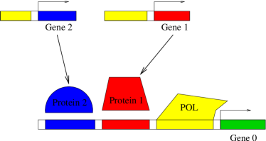
Figure 1: Cartoon of transcriptional regulation of gene 0 by two the transcription factors protein 1 and protein 2.

If we knew the gene-regulatory network of an organism, it would be an interesting question to infer the dynamical behaviour and stationary points of these networks to understand the process of cell development and differentiation. In addition, this knowledge would allow us to numerically predict the outcome of genetic interventions, and eventually to identify new drug targets for medical treatment. It is, however, a very complicated, time-consuming and cost-intensive task to experimentally determine the detailed structure of such networks using techniques like gene-knockout, chromatin immuno-precipitation (ChIP) etc. In fact, genome-wide networks are only know for simple organisms like E. coli Alon1 and baker’s yeast Kepes ; Alon2 , whereas for higher organisms only few functional modules are known, see e.g. Davidson ; Albert .

On the other hand, today it is relatively easy to monitor the gene expression on a genome-wide scale, the most important experimental tools here are microarrays (DNA-chips) which measure the simultaneous abundance of tens of thousands of mRNAs, i.e. of the products of the transcription process, which later on get translated into proteins. It seems therefore an enormously interesting task to infer gene-regulatory interactions from expression data using bio-informatics means. Even if such an approach cannot be expected to replace a direct experimental determination of such interactions, it may well serve as a guide to design efficient and focused experiments.

In the literature, various inference algorithms are discussed. A first class deals with relevance networks, measuring the correlation resp. mutual information of the expression of gene pairs RN1 ; RN2 . This approach obviously may include also indirect interactions, since also second or third neighbours in a regulatory network may be correlated. This is taken into account in the algorithm ARACNe Aracne1 ; Aracne2 , which uses information-theoretic arguments to prune all those links which can be explained by indirect interactions. In Bayesian and dynamic Bayesian networks Bayes1 ; Bayes2 ; Bayes3 ; Bayes4 , also the directed structure of causal dependencies between gene expression levels is inferred: A global scoring function is assigned to arbitrary networks, and the highest scoring network is considered to be the best possible inferred network. Unfortunately, finding this network is an NP-hard task, it can reasonably accessed only using heuristic tools (greedy algorithms with restarts, simulated annealing…) which are likely to get trapped in local extrema of the scoring function. A somewhat similar approach are probabilistic Boolean networks PBN1 ; PBN2 which exhaustively scan all gene pairs or triplets in order to see in how far they determine the expression level of an output gene. Even if being polynomial, this algorithm is restricted to relatively few genes and regulatory functions with at most three inputs.

The inference of gene-regulatory networks is unfortunately plagued by serious problems based on the quantity and the quality of available data. Some of the most relevant limitations are listed below:

• The number $M$ of available expression patterns is in general considerably smaller than the number $N$ of measured genes.

• The available information is, in general, incomplete. The expression of some relevant genes may not be recorded, and external conditions corresponding, e.g., to nutrient, mineral, and thermal conditions are not given. Micro-arrays measure the abundance of mRNA, whereas gene regulation works via the binding of the corresponding proteins (transcription factors) to the regulatory regions on the DNA. Protein and RNA concentrations are, however, not in a simple one-to-one correspondence.

• The data are noisy. This concerns biological noise due to the stochastic nature of underlying molecular processes, as well as the considerable experimental noise existing in current high-throughput techniques.

• Micro-arrays do not measure the expression profiles of single cells, but of bunches of similar cells. This averaging procedure may hide the precise character of the regulatory processes taking place in the single cells.

• Non-transcriptional control mechanisms (chromatin remodelling, small RNAs etc.) cannot be taken into account in expression based algorithms.

• A last problem is a conceptual one: Searching for dependencies between the expression levels of genes does not automatically imply their direct physical interaction in transcriptional regulation. To give an example, strongly coregulated genes may appear as good predictors of each other, without having any direct interaction.

The listed points obviously lead to a limited predictability of even the most sophisticated algorithms. It is therefore very important to test various algorithms on the basis of well described data sets containing some or all of the before-mentioned problems: Only a critical discussion on artificial data sets allows for a sensible interpretation of the algorithmic outcomes when run on biological data.

In this paper, we present a recently introduced statistical-physics motivated inference algorithm build on a message-passing technique which, in a sense, is equivalent to the Bethe-Peierls approximation of statistical physics BP-infer ; Japan . We further use statistical-physics tools, more precisely the replica method developed in the theory of disordered systems and spin glasses, to characterise the performance of this algorithm on artificially generated data, and to compare it to relevance resp. ARACNe networks. We will show that the message-passing technique is able to take into account also collective effects in the common action of various transcription factors, and therefore it outperforms local pair-correlation based algorithms.

The structure of the paper is as follows: In the following section, we formalise the network inference problem. In the third section, we review two types of inference algorithms, namely pair-correlation based methods and a message-passing technique. Than we introduce a generator for artificial data and perform first numerical tests. Sec. V contains a statistical-mechanics approach to the performance of both algorithms, and a careful analysis of their behaviour under various (artificial data) conditions. At the end, we conclude this work, and discuss extensions of the message passing techniques which are necessary for a successful application to biological data.

II The network inference problem

Let us first formalise the network-inference problem. Given are stationary points of the regulatory network, or gene-expression profiles (Note: Temporary expression data can be learnt with a modification of the presented algorithm. Here we concentrate fully on static data.) They can be written in the following form

$$x_{i}^{\mu},\hskip 28.45274pti=0,...,N,\ \ \mu=1,...,M$$ (1)

with $i$ enumerating the considered genes, and $\mu$ the different expression patterns (profiles). In this work, we assume the expression values to be binarized, $x_{i}^{\mu}=-1$ signifies that gene $i$ has very low expression in patterns $\mu$, whereas a high expression is denoted by $x_{i}^{\mu}=1$. Note that we use an Ising spin notation instead of a more standard Boolean one, but this choice will render the technical presentation better accessible. Such a binary representation seems to be oversimplified since gene expression is characterised by mRNA concentrations, but it is applied successfully in various biological examples Davidson ; Albert ; PBN2 . It is expected to work pretty well since gene-regulatory functions show frequently a switch like behaviour Hwa . The simplest examples, repression and activation by a single TF, are illustrated in Fig. 2.

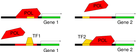
Figure 2: Schematic representation of transcriptional repression (left) and activation (right). Repression works via the competitive binding of POL and the TF to overlapping binding sites, wheres activation uses a short-range attraction between POL and TF when attached to close-by binding sites.

At this level, the inference problem can be considered to factorise over the output variables: We can first reconstruct the regulators for variable 0, then for variable 1 etc. until we reach variable $N$. In our presentation we concentrate therefore to one of these subproblems: Without loss of generality, we are interested in the question in how far and in which way gene 0 is regulated by the genes 1,…,N. We can distinguish two subsequent subproblems

• Topology: Which genes do influence gene 0, and which other genes do not influence gene 0. This result of this question are directed links from the regulating genes to the regulated gene 0.

• Functionality: How do these genes influence the expression of 0? Here we want to restrict this question to the simplest types of interactions, classifying the input genes 1,…,N as activators, repressors or irrelevant for gene 0.

Note that the factorised approach may be oversimplified if experimental noise is considered. Here we are, however, not interested in giving a biologically realistic modelling, but in a theoretical analysis of the proposed message-passing algorithm. We therefore keep this assumption since it allows a more elegant and clear presentation of the results.

As mentioned, we aim at classifying the directed interactions from gene $i$ to gene 0 by a ternary variable,

$$J_{i}=\left\{\begin{array}[]{rl}-1&{\mbox{ if gene $i$ represses the expression of gene 0}}\\ 0&{\mbox{ if gene $i$ does not regulate gene 0}}\\ 1&{\mbox{ if gene $i$ activates the expression of gene 0}}\end{array}\right.$$ (2)

Again, this classification is oversimplified with respect to biological reality. First, it does not include the fact that there may be strong and weak activators or inhibitors, all of them are just characterised by one single variable. Second, there may be interactions where a gene changes its activating or inhibiting character in the presence of other genes. To give an example, the XOR function of two variables cannot be represented within the above-mentioned classification.

It would be possible to overcome this simplification by introducing more complicated variables. On the other hand, this would increase the number and complexity of the model-parameters, and consequently the risk of overfitting. The task of extracting a good predictor from few noisy data requires the model to depend on as few paramters as possible.

To infer this interaction vector, we have also to set up a minimal functional model for the joint interaction of all relevant input genes. Having classified the input genes by this ternary variable, we can sum up the total influence of an expression pattern $\vec{x}=(x_{1},...,x_{N})$ on gene 0. If it overcomes some threshold $\theta$ (which, for clarity of notation, we set to zero in the following), the expression of gene 0 is expected to be enhanced, below this threshold the expression level of gene 0 is repressed. At the Boolean level, we can therefore model the regulatory interaction by the threshold function

$$x_{0}={\rm sign}\left(\sum_{i=1}^{N}J_{i}x_{i}\right)\ .$$ (3)

Note that, slightly more than one decade ago, this function has found considerable attention in statistical physics in the context of the theory of artificial neural networks HeKrPa ; EnBr , it describes a diluted perceptron. In fact, the technical approach presented below consists of an adaption of the well-known Gardner calculus of perceptron learning Ga to the gene-regulatory problem.

Using this model, we are looking for classification vectors $\vec{J}=(J_{1},...,J_{N})$ which are as compatible as possible with the input data $\vec{x}^{\mu},\ \mu=1,...,M$. We therefore introduce a Hamiltonian

$${\cal H}(\vec{J})=\sum_{\mu=1}^{M}\Theta\left(-x_{0}^{\mu}\cdot\sum_{i=1}^{N}J_{i}x_{i}^{m}\right)$$ (4)

which counts the number of patterns whose output contradicts the model (3). The $\Theta$ symbolises the step function, which jumps from zero for negative arguments to one for non-negative arguments. One aim of the algorithm will be to minimise this Hamiltonian.

To get reasonable results, we will also implement another biologically motivated constraint. Gene regulatory networks are diluted, i.e. the number of transcription factors for one gene is generally restricted to a small number. In the best known regulatory network, the one of bakers yeast, one finds evidence that the number of genes regulating commonly one gene is distributed according to a narrow exponential distribution, which can be explained by physical constraints for the positioning of transcription factor binding sites. To take into account this diluted character, we will also control the number

$$N_{eff}(\vec{J})=\sum_{i=1}^{N}\left(1-\delta_{J_{i},0}\right)$$ (5)

of effectively present, i.e., non-zero links via a conjugated external field. This a priori bias towards diluted graphs helps again to avoid overfitting of the data, since it reduced the entropy of the search space.

This idea is closely related to methods of regression and graphical-model selection using $\ell_{1}$-parameter regularization discussed in the machine-learning literature. The original idea was developped by Tibshirany for the case of sparse regression in linear models tibshirany , but it can be extended to more general convex optimization problems wainwright ; banerjee ; koller ; schmidt . In all these cases, the optimization of the cost function is restricted by the $\ell_{1}$-norm $\sum_{i}|J_{i}|$ of the model parameters $J_{i}$. The cusp-like structure of this constraint in $J_{i}=0$ forces a part of the parameters to be exactly zero. In the presence of sufficient data this method can be shown to asymptotically reproduce the correct topological structure of the underlying model meinshausen . In principle, one could use any $\ell_{n}$-norm $\sum_{i}|J_{i}|^{n}$ for regularizing parameters. However, only for $0\leq n\leq 1$ some of the optimal parameters assume values equal to zero; for $1\leq n$ the constraint is convex, thus it can be added to the cost function without destroying its convexity. Only the $\ell_{1}$-norm fullfils both conditions.

Our case is, however, different from these examples. The discrete nature of the model parameters renders the model a priori NP-hard, and convex optimization cannot be applied. Furthermore, we are interested in ensembles of possible networks rather than a single network as predicted by convex optimization.

III Inference algorithms

In this section, we present two classes of inference algorithms. The first one is based on pairwise correlations between the output variable $x_{0}$ and inputs $x_{i}$. This correlation can be measured in different ways, two of the most important measures are the connected correlation coefficient (or its normalised version, the Pearson correlation coefficient), and the mutual pairwise information of the two variables. Inference algorithms based on this measure are wide spread, in their simplest version they result in the so-called co-expression or relevance network. Such networks normally contain much more links than the actual regulatory interaction between transcription factors and regulated genes: Also second neighbours may still be considerably correlated. This is taken into account in a very clever way in the algorithm ARACNE which eliminates all those links which, from an information theoretic point of view, can be explained via a two-step interaction with an intermediate variable. This elimination step increases strongly the precision of the algorithm since it reduces the number of false positives, but it decreases also its sensitivity cancelling many weak pair interactions.

The second method is the central one of our paper. It is based on a message-passing algorithm (more precisely a belief-propagation algorithm) which characterises the statistical properties of the set of all potential coupling vectors, weighted with respect to Hamiltonian (4) and the number of relevant links (5). We will see that this method is able to - at least partially - recognise the collective effects between different inputs in the data-generating rule (20). It therefore goes beyond simple two-point correlations, at the cost of being related to a more specific model of gene regulation.

Both algorithms will output a ranking of all potential input variables $1,...,N$ according to the considered significance measure, going from the most significant genes to the most insignificant ones. The method itself has no intrinsic criterion where to cut this list. It his, however, possible to use suitable data randomisation procedures which give an indication at which level the significance value of an input may be explained by a random input-output relation (more precisely one may assign a $p$-value giving the probability that the significance value or a larger one comes from a random input-output relation).

III.1 Relevance networks

Let us first explain pair-correlation based methods, like relevance networks RN1 ; RN2 . They are based on measuring the correlation between the output variable $0$ and each input variable $i\in\{1,...,N\}$. The central quantities hereby are the joint distribution $p(x_{0},x_{i})$ of the two variables, as estimated from the data via

$$p(x_{0},x_{i})\simeq\frac{1}{M}\sum_{\mu=1}^{M}\delta(x_{0},x_{0}^{\mu})\ \delta(x_{i},x_{i}^{\mu})\ ,$$ (6)

and its marginals

$$p(x_{0}) = \sum_{x_{i}}p(x_{0},x_{i})\ \simeq\ \frac{1}{M}\sum_{\mu=1}^{M}\delta(x_{0},x_{0}^{\mu})$$

$$p(x_{i}) = \sum_{x_{0}}p(x_{0},x_{i})\ \simeq\ \frac{1}{M}\sum_{\mu=1}^{M}\delta(x_{i},x_{i}^{\mu})\ .$$ (7)

The central question is, in how far the two variables are correlated, i.e. in how far the joint distribution is different from the factorised distribution $p(x_{0})p(x_{1})$. This can be measured either via the connected correlation coefficient,

$$C_{0i}=\sum_{x_{0},x_{1}}\left[p(x_{0},x_{i})-p(x_{0})p(x_{i})\right]\ x_{0}\ x_{i}\ ,$$ (8)

or via the mutual information,

$$I_{0i}=\sum_{x_{0},x_{1}}p(x_{0},x_{i})\log\frac{p(x_{0},x_{i})}{p(x_{0})p(x_{i})}\ .$$ (9)

Note that Eq. (8) is equivalent to the standard definition of the connected correlation, but the present formulation brings to evidence the distance measure between the joint and the factorised probabilities. The mutual information is also known as the Kullback-Leibler divergence between $p(x_{0},x_{i})$ and $p(x_{0})p(x_{i})$. It equals zero if and only if both are equal, i.e. if $x_{0}$ and $x_{i}$ are statistically independent, and it is positive otherwise.

These numbers (or, in the case of the correlation coefficient its absolute value) can be ordered and give thus a ranking of the inputs according to their statistical correlation with the output. One can expect the most significant correlations to come from direct interactions, whereas weak correlations are a sign for a non-existing link in the data-generating system (model or experiment).

Note that this method is not able to detect the directed character of gene regulatory interactions, since the very definition in Eq. (8) is symmetric against exchange of variables $0$ and $i$. This is a major drawback of correlation based methods, and can be eliminated using the algorithm proposed in the next subsection.

III.2 Belief propagation for network inference

In this section we present our message-passing algorithm for network inference. It has two major differences to the correlation based method presented before. On one hand, it is model based (cf. Eq. (3)) and therefore may fail in situations where this model is not sufficiently well-adapted. On the other hand, this model-based approach allows to take into account the joint action of all potential regulator variables. Therefore it may well go beyond the simple two-point correlations used in the previous section.

The basic step is the introduction of a global weight function

$$W(\vec{J}\ )=\exp\left\{-\beta{\cal H}(\vec{J})-hN_{eff}(\vec{J})\right\}$$ (10)

weighing all candidate coupling vectors $\vec{J}$ (i.e., all potential regulatory networks) with respect to their energy ${\cal H}(\vec{J})$ and the number $N_{eff}(\vec{J})$ of non-zero coupling components, see Eqs. (4,5) for the definitions. This weight depends on two not yet specified parameters: The formal inverse temperature $\beta$ controls the energy. In the limit $\beta\to\infty$ the weight concentrates in the global minima of ${\cal H}$. The formal external field $h$ controls, on the other hand, the density of non-zero entries in $\vec{J}$. Due to the biologically reasonable request for diluted $\vec{J}$, we expect this field to assume high values. There is no obvious strategy of fixing these two parameters, but we will describe a reasonable heuristic strategy.

Note that the data $\vec{x}^{\mu}$ represent the quenched disorder, whereas the $N$ components of the vector $\vec{J}$ are the (ternary) degrees of freedom. The primary algorithmic aim here is to determine the marginal single-site distributions

$$P_{i}(J_{i})\propto\sum_{\{J_{j}\in\{0,\pm 1\};j\neq i\}}W(\vec{J})$$ (11)

where the normalisation constant in this equation is, as usually, given by the partition function. A direct calculation of these marginals is a computationally intractable task, since Eq. (11) contains the sum over $N-1$ ternary degrees of freedom, i.e. we have to sum up $3^{N-1}$ terms. It is therefore necessary to find some - possibly heuristic - tools which render this task efficiently solvable.

Here we use the idea of message-passing (MP) techniques. These were initially created for problems with sparse constraints, i.e., variables have to be contained in few constraints, and constraints have to contain few variables. Typical examples for such problems are random 3-SAT and colourings or vertex covers on finite-connectivity random graphs. Here we are in the opposite situation: Each variable $J_{i}$ is contained in $M$ constraints given by the expression patterns $\vec{x}^{\mu},\mu=1,...,M$, and each constraint contains all $N$ variables. Recently the applicability of BP has, however, been verified in a number of cases ranging from information theory to perceptron learning CDMA ; UdKa ; BrZe . In BP-infer ; Japan we have adopted these techniques to the specific needs of our network-inference problem.

The BP equations can be easily written down. Each constraint sends a message to each variable, and each variable sends a message to each constraint:

$$P_{i\to\mu}(J_{i}) \propto e^{-h|J_{i}|}\ \prod_{\nu\neq\mu}\rho_{\nu\to i}(J_{i})$$

$$\rho_{\mu\to i}(J_{i}) \propto \sum_{\left\{J_{j},\ j\neq i\right\}}\exp\left\{-\beta\Theta\left[-x_{0}^{\mu}\cdot\sum_{k}J_{k}x_{k}^{\mu}\right]\right\}\prod_{j\neq i}P_{j\to\mu}(J_{j})$$ (12)

The messages have an intuitive interpretation. The variable sends the information to the constraint: “If you were not present, I would have the statistical properties given by $P_{i\to\mu}(J_{i})$.” The constraint, on the other hand, sends a message to the variable: “Seen the behaviour of the other variables, please behave according to $\rho_{\mu\to i}(J_{i})$ in order to satisfy me.” Note that there are $2MN$ of these messages, which form a self-consistently closed set of equations. The true marginal distribution can than be estimated from the messages sent by all constraints,

$$P_{i}(J_{i})\propto e^{-h|J_{i}|}\ \prod_{a}\rho_{a\to i}(J_{i})\ .$$ (13)

From a computational point of view, we still have not gained anything. The second of Eqs. (III.2) still contains the exponential sum over all but one $J_{j}$. This problem can be solved by the following observation: The dependence on the $J_{i}$ enters via $\sum_{k}J_{k}x_{k}^{\mu}$ and via the factorized distribution $\prod_{j\neq i}P_{j\to\mu}(J_{j})$. For $N\gg 1$ we can apply the central limit theorem and replace the sum over the $N-1$ couplings by a single Gaussian integral, for finite $N$ it will be used as a computationally efficient approximation. We replace the second line of Eqs. (III.2) by

$$\rho_{\mu\to i}(J_{i})\propto\int_{-\infty}^{\infty}\frac{dh}{\sqrt{2\pi}\Delta_{\mu\to i}}\exp\left\{-\frac{(h-h_{\mu\to i})^{2}}{2\Delta_{\mu\to i}^{2}}-\beta\Theta\left[-x_{0}^{\mu}\cdot(J_{i}x_{i}^{\mu}+h)\right]\right\}$$ (14)

with

$$h_{\mu\to i} = \sum_{j\neq i}x_{j}^{\mu}\ \langle J_{j}\rangle_{j\to\mu}$$

$$\Delta_{\mu\to i}^{2} = \sum_{j\neq i}\ {x_{j}^{\mu}}^{2}\left(\ \langle J_{j}^{2}\rangle_{j\to\mu}-\langle J_{j}\rangle_{j\to\mu}^{2}\ \right)$$ (15)

where $\langle\cdot\rangle_{j\to\mu}$ denotes the average over $P_{j\to\mu}(J_{j})$. Due to the step-like shape of the Heaviside function, the right-hand site in Eq. (14) can be expressed via the sum of two error functions, which again leads to a faster numerical implementation.

Note that, in contrast to what happens in most combinatorial optimisation problems (and, in particular, also in Bayesian and dynamic Bayesian network learning), we do not have the aim to construct one single instance of a “good” coupling vector $\vec{J}$, because this vector may be quite different from the original data-generating vector. We are instead interested in characterising the ensemble of all sets of vectors. More precisely, the marginal probability $P_{i}(J_{i})$ gives us a confidence measure for the hypothesis that the output variable $x_{0}$ actually depends on $x_{i}$: It measures the fraction of all suitable coupling vectors $\vec{J}$ (as weighted by Eq. (10)) where the entry $i$ takes value $J_{i}$. We can therefore base a global ranking of all potential couplings in the probability $(1-P_{i}(J_{i}=0))$ of having a non-zero coupling (or alternatively on the average coupling $\langle J_{i}\rangle_{i}$).

Having calculated the messages and the marginal distributions, we may determine the energy of the average coupling vector

$$E=\sum_{\mu=1}^{M}\Theta\left(-x_{0}^{\mu}\cdot\sum_{i=1}^{N}\langle J_{i}\rangle_{i}\ x_{i}^{m}\right)$$ (16)

and the Bethe entropy

$$S=\sum_{\mu=1}^{M}S_{\mu}-(N-1)\sum_{i=1}^{N}S_{i}\$$ (17)

characterising the number of “good” coupling vectors. In the last expression, the site entropy $S_{i}$ is given by

$$S_{i}=-\sum_{J_{i}=-1,0,1}P_{i}(J_{i})\ \ln P_{i}(J_{i})\ ,$$ (18)

and the pattern entropy

$$S_{\mu} = -\sum_{\vec{J}}P_{\mu}(\vec{J}\;)\ \ln P_{\mu}(\vec{J}\;)$$ (19)

$$P_{\mu}(\vec{J}\;) = \exp\left\{-\beta\Theta\left[-x_{0}^{\mu}\cdot\sum_{k}J_{k}x_{k}^{\mu}\right]\right\}\prod_{i}P_{i\to\mu}(J_{i})$$

can be calculated in analogy to $\rho_{\mu\to i}$ via a Gaussian approximation of the sum over $\vec{J}$.

So far, we did not fix the parameters $\beta$ and $h$ controlling the energy and the dilution of the inferred vectors. A simple heuristic strategy is the following: Fix the number $N_{eff}(\vec{J}\ )$ externally to some desired value, and start at high temperature and initial $h$ given by $N_{eff}=2\cosh h/(1+2\cosh h)$. Update the messages starting from some random initialisation, and calculate the energy of the average coupling vector and the Bethe entropy. Now decrease the temperature gradually towards the zero-entropy (or zero energy), adapting $h$ such that $N_{eff}(\vec{J}\ )$ remains close to the desired value. This strategy can be repeated for various values of $N_{eff}$. In practical applications, also an optimal $N_{eff}$ can be determined by first dividing the data set into a training and a test set, calculating the marginal probabilities on the training set, and minimising the corresponding prediction error of the average coupling vector on the test set. In the case of artificial data coming from a known coupling vector, we can train on all data and compare directly with the correct vector.

IV Tests on artificial data

Before coming to a theoretical analysis of the algorithmic performance, we make some numerical test to get a first impression of the predictive power of the two algorithms.

IV.1 The data generator

In order to check and compare the performance of the algorithms presented below, we have to introduce a data generator. It allows to create data sets with well-controlled properties, and the knowledge about the data-generating rule allows to compare the results of the inference algorithm to the true rule.

In this work, we concentrate on data generated by a simple threshold function with couplings $J_{i}^{0}$,

$$x_{0}^{\mu}={\rm sign}\left(\sum_{i=1}^{N}J_{i}^{0}x_{i}^{\mu}+\eta^{\mu}\right)$$ (20)

for all $\mu-1,...,M$. The inputs $\vec{x}^{\mu}=(x_{1}^{\mu},...,x_{N}^{\mu})$ have independently distributed binary entries. With respect to the ternary classification into activators, repressors and non-interacting genes, this rule has two major differences

• Heterogeneity: The couplings $J_{i}$ may take values which are different from $0,\pm 1$. This allows to introduce regulatory variables of different interaction strengths, i.e. in particular weak and strong activators resp. repressors. In this work, we will study in particular the case where $J_{i}\in\{0,\pm 1,\pm 2\}$. The couplings itself will be drawn randomly and independently with respect to a distribution

  $$\rho(J_{i}^{0})=(1-k_{1}-k_{2})\delta(J_{i}^{0})+\frac{k_{1}}{2}[\delta(J_{i}^{0}+1)+\delta(J_{i}^{0}-1)]+\frac{k_{2}}{2}[\delta(J_{i}^{0}+2)+\delta(J_{i}^{0}-2)]$$ (21)

  Generalisations will be straight-forward, but they do not alter at all the conclusions of this work. Note that real gene-regulatory networks are sparse, i.e. we have to work in the regime $k_{1,2}\ll 1$. In the statistical mechanics calculations presented below, we will consider the thermodynamic limit $N\to\infty$. At a first glance it seems to be reasonable to assume the usual scaling of finite-connectivity graphs, $k_{1,2}={\cal O}(N^{-1})$, for the coupling probabilities. Due to technical reasons we will, however, concentrate on the scaling $k_{1,2}={\cal O}(1)\ll 1$. This choice will be justified by comparison with numerical data.

• Noise: In biological data, there are various kinds of noise. The first one is biological noise resulting from the stochastic nature of cellular processes. The second and more annoying one is experimental noise which is strongly present in most high-throughput data. In addition, biological data are normally incomplete in the sense, that not all existing gene expression levels are measured, that nutrient or mineral concentrations, temperature and other external factors are not recorded etc. In our data generator, we have included a simple additive noise term $\eta^{\mu}$ which we assume to be independent for various patterns $\mu$. More precisely we assume it to be Gaussian with

  $$\overline{\eta}^{\mu} = 0$$

  $$\overline{\eta^{\mu}\eta^{\nu}} = \gamma N\delta_{\mu,\nu}$$ (22)

  for all $\mu,\nu\in\{1,...,M\}$. Note that the scaling of the variance with $\sqrt{N}$ makes the noise to be of the same order of magnitude as the signal $\sum J^{0}_{i}x_{i}^{\mu}$. For the special case $\gamma=k_{1}+4k_{2}$, both noise and signal have exactly the same statistical properties.

Note that this data generation rule is more complex than the inference rule (3). This will result in non-feasible data, i.e., a non-zero “energy” ${\cal H}(\vec{J})$ even for the best inferred couplings $\vec{J}$. The best possible result would be $J_{i}={\rm sign}J_{i}^{0}$ (here with ${\rm sign(0)=0}$) since this would correctly assign the attributes activating, repressing, irrelevant to the couplings. Due to the presence of noise as well as due to the finite amount of data available, such a perfect prediction will be impossible. We therefore introduce the following notation

$$\begin{array}[]{lll}J_{i}^{0}=0&J_{i}=0&{\mbox{ true negative (TN)}}\\ J_{i}^{0}\neq 0&J_{i}=0&{\mbox{ false negative (FN)}}\\ J_{i}^{0}=0&J_{i}\neq 0&{\mbox{ false positive (FP)}}\\ J_{i}^{0}\neq 0&J_{i}\neq 0&{\mbox{ true positive (TP)}}\end{array}$$ (23)

It can be refined taking also into account the relative sign of the original and the inferred coupling, cf. the above discussion about topology and functionality. One of the aims is to predict a fraction of all couplings with high precision, i.e. to have an as high as possible number of TP with a low number of FP. The quality measure we use will be the confrontation of the recall, or sensitivity,

$$RC=\frac{N_{TP}}{N_{TP}+N_{FN}}$$ (24)

and of the precision, or specificity,

$$PR=\frac{N_{TP}}{N_{TP}+N_{FP}}\ .$$ (25)

The recall describes the fraction of all existing non-zero couplings which are predicted by the algorithm, whereas the precision tells us which fraction of all predicted links is actually present in the data generator.

IV.1.1 Feasible data

As a first test, we have run BP on data sets with $k_{2}=\gamma=0$. In this case, also the couplings of the data generator function assume only the three values $J_{i}^{0}\in\{0,\pm 1\}$, and noise is absent. This means that the data set is feasible, the model (3) on which we base our inference is able to reproduce the data without errors. We therefore work automatically at zero formal temperature, and thus at zero energy.

The difficulty of the test problem comes from the fact that we are using an extremely sparse coupling vector: Only 3 out of $N=600$ input variables are coupled to the output via a non-zero coupling $J_{i}^{0}$. We also present relatively small data sets with $M\leq 70$. Is BP able to recognise the three important input variables?

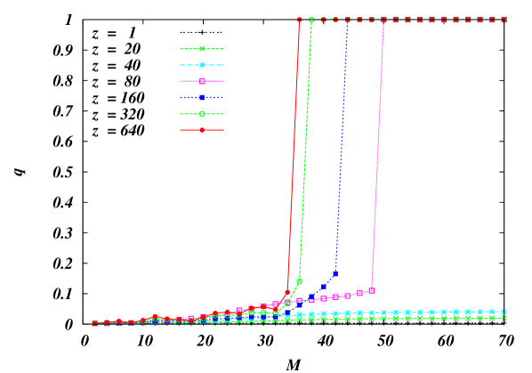
Figure 3: Network inference from a feasible data set: Displayed are the overlap between the generator and the BP output as a function of the number of presented patterns, for various values of $z=e^{h}$. The data generator has $N=600$ inputs, but only 3 are non-zero. Curves correspond to one single test sample.

First, we have done experiments without the exterior diluting field $h$. The results are given in Fig. 3, where the quality of the prediction is measured by the overlap

$$q=\frac{1}{|\vec{J}^{0}|^{2}}\sum_{i=1}^{N}\sum_{J_{i}}J_{i}^{0}J_{i}P_{i}(J_{i})\ .$$ (26)

This overlap takes for all considered numbers $M$ of presented patterns only very small values, the algorithm is not able to recognise the relevant inputs. The situation changes drastically, if we add the diluting field $h$. We find, at some $h$-dependent point, a discontinuous jump from a very bad BP solution with small overlap to a perfectly polarised solution with $q=1$. The algorithm has perfectly recognised the relevant three inputs, and thus perfectly reconstructed the data generating rule! The number of needed patterns decreases with $h$, and can be as small as $M=35$ for large fields.

For even larger fields, the algorithm runs into problems: The dilution becomes as important for the algorithm as the energy constraints, and the BP solution polarises completely to the vector $J_{i}\equiv 0$. Best performance is obtained for fields just below this point.

IV.1.2 Unfeasible data

The success of BP for feasible data sets encourages us to go ahead to more involved cases, i.e., cases with heterogeneities in the coupling strength ($k_{1},k_{2}\neq 0$) and possibly with noise ($\gamma\neq 0$). Here we give a first example of a data generator with $N=600$ inputs, but only 30 of them have a non-zero coupling to the output - 15 of them with an absolute value equal to two, 15 with absolute value one ($k_{1}=k_{2}=0.025$). We generate $M=300$ patterns and apply both inference algorithms. The resulting rankings can be cut at arbitrary points, such that we can measure a recall-vs.-precision curve as given in Fig. 4.

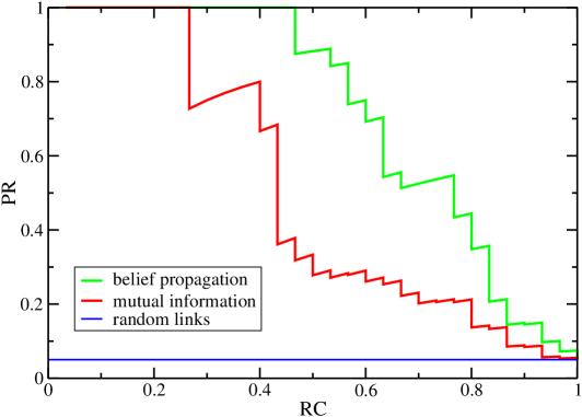
Figure 4: Precision versus recall for inference with BP (green line) and via pairwise mutual information (red line). The parameters of the model are $N=600,M=300$ and $k_{1}=k_{2}=0.025$, corresponding to 15 strong links ($J^{0}=\pm 2$) and 15 weak links ($J^{0}=\pm 1$), noise is absent. The dilution value of BP is chosen to be slightly smaller than the initial dilution, $n_{eff}=0.037$.

We find that both algorithms start at precision one for the highest ranking inputs. The algorithm based on mutual information includes, however, the first false positive after 8 true positives, whereas BP is able to find the first 14 true positives before including the first erroneous link. Also later on the performance of BP remains well above the one of the MI. Note that most of the initially recognised links are strong activators or repressors, only one of the first 14 true positives in BP is an activator with $J_{i}^{0}=1$. Stronger signals are obviously detected first.

Even if not being perfect, it is to be noted that both algorithms perform much better than a random ranking which would fluctuate around an average precision of only $PR=k_{1}+k_{2}=0.05$, as marked by the blue line in the figure.

V A statistical analysis of the algorithmic performance

Can we explain this behaviour analytically? Can we understand the discontinuous transition from very bad to perfect inference in the case of a feasible data set? Can we understand the relative behaviour of BP compared to the different pair-correlation based methods?

In the following we will first calculate exactly the precision-versus-recall curve for the correlation coefficient and the mutual information, and than we go to an analysis of the BP performance via a statistical mechanics analysis of the Gibbs weight given in Eq. (10). In both cases, we are mainly interested in the thermodynamic limit $N\to\infty$. In this limit, we also consider $M$ to diverge, with $\alpha=M/N$ being asymptotically constant. The probabilities $k_{1}$ and $k_{2}$ for non-trivial couplings in the data generator are considered to be finite, i.e. non-trivial couplings constitute a finite fraction of all entries of $\vec{J}^{0}$.

V.1 Pair correlation and mutual information

Let us recall the estimate of the joint distribution of the values of variable 0 and variable $i$ as calculated from the data. Using Eq. (6), and plugging in Eq. (20) for the value of the outputs $x_{0}^{\mu}$, we get

$$p(x_{0},x_{i})=\frac{1}{M}\sum_{\mu=1}^{M}\delta(x_{0},{\rm sign}[\vec{J}^{0}\cdot\vec{x}^{\mu}+\eta^{\mu}])\ \delta(x_{i},x_{i}^{\mu})\ .$$ (27)

Due to the random nature of the input patterns, this quantity itself is a random variable with some distribution ${\mathbf{P}}(p(x_{0},x_{i}))$. Since the different patterns are statistically independent, the joint probability results as a sum over $M=\alpha N$ independently and identically distributed variables. According to the central limit theorem, ${\mathbf{P}}(p(x_{0},x_{1}))$ is thus Gaussian. Its mean can be calculated as

$$\overline{p(x_{0},x_{i})} = \frac{1}{2^{N}}\sum_{x_{1}^{1},...,x_{N}^{1}}\delta(x_{0},{\rm sign}[\vec{J}^{0}\cdot\vec{x}^{1}+\eta^{1}])\ \delta(x_{i},x_{i}^{1})$$ (28)

$$= \frac{1}{2^{N}}\sum_{\{x_{j}^{1};j\neq i\}}\delta\left(x_{0},{\rm sign}\left[J_{i}^{0}x_{i}+\sum_{j\neq i}J_{j}^{0}x_{j}^{1}+\eta^{1}\right]\right)$$

where we have used that the input variables are independent and unbiased, and that the mean of all $M$ contributions to the sum is identical. For calculating this sum, we use another time the central limit theorem, the sum $y=\sum_{j\neq i}J_{j}^{0}x_{j}^{1}$ is Gaussian distributed with mean zero and second moment

$$\overline{y^{2}}=(k_{1}+4k_{2}+\gamma)N+{\cal O}(1)=:\Delta_{y}^{2}\ .$$ (29)

We thus get

$$\overline{p(x_{0},x_{i})} = \frac{1}{2}\int_{-\infty}^{\infty}\frac{dy}{\sqrt{2\pi}\Delta_{y}}e^{-y^{2}/(2\Delta_{y}^{2})}\ \delta\left(x_{0},{\rm sign}[J_{i}^{0}x_{i}+y]\right)$$ (30)

$$= \frac{1}{2}\ H\left(-\frac{J_{i}^{0}x_{0}x_{i}}{\sqrt{(k_{1}+4k_{2}+\gamma)N}}\right)$$

with $H(x)=\int_{x}^{\infty}\frac{dy}{\sqrt{2\pi}}e^{-\frac{y^{2}}{2}}$. We expand this function around zero, and find

$$\overline{p(x_{0},x_{i})}=\frac{1}{4}+\frac{J_{i}^{0}x_{0}x_{i}}{2\sqrt{2\pi(k_{1}+4k_{2}+\gamma)N}}+{\cal O}(N^{-1})\ .$$ (31)

The calculation of the variance is now straight-forward. We have

$$\overline{p(x_{0},x_{i})^{2}}=\frac{M-1}{M}\ \overline{p(x_{0},x_{i})}^{2}+\frac{1}{M}\ \overline{p(x_{0},x_{i})}\ ,$$ (32)

and consequently we find

$$\overline{[\Delta p(x_{0},x_{i})]^{2}} = \frac{1}{M}\ \overline{p(x_{0},x_{i})}\ (1-\overline{p(x_{0},x_{i})})$$ (33)

$$= \frac{3}{16\alpha N}+{\cal O}(N^{-3/2})\ .$$

Finally we need the correlation for different value pairs $(x_{0},x_{i})\neq(x^{\prime}_{0},x^{\prime}_{i})$. Following the the same strategy as before, we find

$$\overline{\Delta p(x_{0},x_{i})\ \Delta p(x^{\prime}_{0},x^{\prime}_{i})}=-\frac{1}{16\alpha N}+{\cal O}(N^{-3/2})\ .$$ (34)

A side remark is necessary here. The covariance matrix of all four values of $p(x_{0},x_{i})$ is degenerate, with a zero-eigenvector $(1,1,1,1)$. It is, however, clear that all four quantities cannot have a simple joint Gaussian distribution - given three, the fourth is determined by normalisation, $\sum_{x_{0},x_{i}}p(x_{0},x_{i})=1$. The zero-eigenvector thus corresponds to the forbidden normalisation breaking fluctuations.

V.1.1 Pair correlations

Let us, however continue with the pair correlations between the output variable $x_{0}$ and a potential regulator $x_{i}$. We write

$$C_{0i} = \sum_{x_{0},x_{i}}p(x_{0},x_{i})\ x_{0}x_{i}$$ (35)

$$= p(1,1)+p(-1,-1)-p(1,-1)-p(-1,1)$$

$$= 2\ p(1,1)+2\ p(-1,-1)-1$$

where, in the last line, we have exploited the normalisation of $p(x_{0},x_{1})$. Due to imperfect sampling in a finite data set, this is again a Gaussian random variable. Using Eq. (31) we find its mean to be

$$\overline{C_{0i}}=\frac{2J_{i}^{0}}{\sqrt{2\pi(k_{1}+4k_{2}+\gamma)N}}+{\cal O}(N^{-1})\ ,$$ (36)

whereas its variance can be calculated directly from Eqs. (33) and (34),

$$\overline{(\Delta C_{0i})^{2}}=\frac{1}{\alpha N}+{\cal O}(N^{-3/2})\ .$$ (37)

Both mean and variance scale as ${\cal O}(N^{-1/2})$, introducing thus $\tilde{C}_{0i}=\sqrt{N}\ C_{0i}$ we find its probability distribution

$$P(\tilde{C}_{0i}|J_{i}^{0})=\sqrt{\frac{\alpha}{2\pi}}\exp\left\{-\frac{\alpha}{2}\left(\tilde{C}_{0i}-\frac{2J_{i}^{0}}{\sqrt{2\pi(k_{1}+4k_{2}+\gamma)}}\right)^{2}\right\}$$ (38)

conditioned to the value of the coupling $J_{i}^{0}$ between variables $0$ and $i$ in the data generator (20). At this point, one recognises the potential and also the limitations of network inference via pair correlations: The mean value of the correlations of different variables is well separated by a term being proportional to the coupling strength, and in particular strong activators and inhibitors should be distinguishable from irrelevant variables. On the other hand, the variance of distribution (38) is of the same order of magnitude as the mean, i.e. the distributions for different values $J_{i}^{0}$ overlap, and errors in the network inference are unavoidable. The only way to suppress errors is to augment the amount of data, the variance of the measured correlation values around its expectation decays as $1/\sqrt{\alpha}$.

The measured pair correlations, or more precisely their absolute values, serve as a ranking for the inclusion of different variables into the reconstructed network. Let us therefore imagine that we introduce a cutoff $\theta>0$ for the absolute value of the rescaled correlations $C_{0i}$, i.e., for all $i$ with $|\tilde{C}_{0i}|>\theta$ we introduce a coupling, for all inputs with a smaller absolute correlation value we assume the coupling to be absent. The fraction of included couplings with given original $J^{0}$ is than found to be

$$P\left(\ |\tilde{C}_{0i}|>\theta\ |\ J^{0}\right) = \int_{-\infty}^{-\theta}d\tilde{C}_{0i}P(\tilde{C}_{0i}|J^{0})+\int_{\theta}^{\infty}d\tilde{C}_{0i}P(\tilde{C}_{0i}|J^{0})$$ (39)

$$= H\left(\sqrt{\alpha}\left[\theta-\frac{2J_{i}^{0}}{\sqrt{2\pi(k_{1}+4k_{2}+\gamma)}}\right]\right)+H\left(\sqrt{\alpha}\left[\theta+\frac{2J_{i}^{0}}{\sqrt{2\pi(k_{1}+4k_{2}+\gamma)}}\right]\right)$$

For $J^{0}\neq 0$, the corresponding included couplings are true positives. For $J^{0}=0$, they are false positives. We thus can write up the recall and the precision of the inferred network, in dependence of the cutoff parameter $\theta$:

$$RC(\theta) = \frac{k_{1}P\left(\ |\tilde{C}_{0i}|>\theta\ |\ \pm 1\right)+k_{2}P\left(\ |\tilde{C}_{0i}|>\theta\ |\ \pm 2\right)}{k_{1}+k_{2}}$$

$$PR(\theta) = \frac{k_{1}P\left(\ |\tilde{C}_{0i}|>\theta\ |\ \pm 1\right)+k_{2}P\left(\ |\tilde{C}_{0i}|>\theta\ |\ \pm 2\right)}{(1-k_{1}-k_{2})P\left(\ |\tilde{C}_{0i}|>\theta\ |\ 0\right)+k_{1}P\left(\ |\tilde{C}_{0i}|>\theta\ |\ \pm 1\right)+k_{2}P\left(\ |\tilde{C}_{0i}|>\theta\ |\ \pm 2\right)}$$ (40)

Changing the value of $\theta$ from high to small values, we increase the recall from zero to one, at the cost of a decreasing precision. More details will be given below, in the comparison to the results of the massage-passing based inference algorithm.

Note that we did not require the correct determination of the sign of the coupling, a generalisation to this case is, however, straight forward. For not too small $\alpha$, it practically does not lead to recognisable differences, i.e. the waste majority all true positives is recognised due to the correct sign of the measured correlation.

V.1.2 Mutual information

In how far does the network reconstruction change if we go from correlations to the pairwise mutual information as given in Eq. (9)? The latter has a nonlinear dependence on the pair correlations $p(x_{0},x_{1})$, and consequently it does not have a Gaussian distribution. We may, however, use the fact that variables are only weakly correlated, and write

$$p(x_{0},x_{i})=\frac{1}{4}+\frac{z(x_{0},x_{i})}{\sqrt{N}}\ .$$ (41)

The newly introduced function $z(x_{0},x_{1})$ contains all non-trivial correlations between $x_{0}$ and $x_{1}$, and it is of ${\cal O}(N^{0})$. Note that at this point we consider Eq. (41) to be an exact definition of $z(x_{0},x_{i})$, i.e. the latter contains all the lower-order corrections in $N$ and not only the dominant term. Due to the normalisation of $p$ it fulfils $\sum_{x_{0},x_{i}}z(x_{0},x_{i})=0$. We further on write for the two marginal single-variable distributions of $p(x_{0},x_{i})$:

$$p(x_{0}) = \frac{1}{2}+\frac{z(x_{0})}{\sqrt{N}}$$

$$p(x_{i}) = \frac{1}{2}+\frac{z(x_{i})}{\sqrt{N}}\ .$$ (42)

Plugging this into the definition of the mutual information, we find

$$I_{0i}=\sum_{x_{0},x_{i}}\left[\frac{1}{4}+\frac{z(x_{0},x_{i})}{\sqrt{N}}\right]\ \left[\log\left(1+\frac{4\ z(x_{0},x_{i})}{\sqrt{N}}\right)-\log\left(1+\frac{2\ z(x_{0})}{\sqrt{N}}\right)-\log\left(1+\frac{2\ z(x_{i})}{\sqrt{N}}\right)\right]$$ (43)

Expanding the logarithm up to second order in the $z$, and using the normalisation to eliminate all linear terms, we find after some straight-forward algebra

$$I_{0i} = \frac{2}{N}\left[z(1,1)+z(-1,-1)\right]^{2}+{\cal O}\left(N^{-\frac{3}{2}}\right)$$ (44)

$$= \frac{C_{01}^{2}}{2}+{\cal O}\left(N^{-\frac{3}{2}}\right)\ .$$

We thus conclude that, at least under the scaling limits considered in this work, the correlation coefficient and the mutual information carry the same information. A network reconstruction algorithm based on either of these two quantities thus leads to the same results.

V.2 Characterising the set of coupling vectors

In the last subsection, we have analytically characterised the performance of a network inference algorithm based on pairwise correlation measures. Is a similar comparison possible for the belief-propagation algorithm introduced in Sec. III.2? As already mentioned, the algorithm is based on the measure

$$P(\vec{J})=\frac{1}{Z(\beta,h)}\exp\left\{-\beta{\cal H}(\vec{J})-hN_{eff}(\vec{J})\right\}$$ (45)

which assigns a weight to every coupling vector $\vec{J}$. This weight depends on its performance on the data set $\{\vec{x}^{\mu}\}$ as measured by the Hamiltonian ${\cal H}(\vec{J})$ defined in Eq. (4), and on the effective number $N_{eff}(\vec{J})$ of relevant inputs $J_{i}\neq 0$ as defined in Eq. (5). A positive inverse temperature $\beta$ introduces a bias toward $\vec{J}$ with few errors on the data set, a positive $h$ favours diluted coupling vectors. The aim of the algorithm was to determine the marginal distributions $P_{i}(J_{i})$ for single entries of the vector $\vec{J}$, and use the probability $P_{i}(J_{i}\neq 0)$ that such a component becomes non-zero for ranking the input variables according to their relevance for the output.

Note that in this way we do not work with a single reconstructed network, which may or may not be similar to the data generator, but with a probability measure over all feasible coupling vectors.

To characterise the performance of this ranking procedure we have to calculate first the partition function

$$Z(\beta,h)=\sum_{\vec{J}\in\{0,\pm 1\}^{N}}\exp\left\{-\beta{\cal H}(\vec{J})-hN_{eff}(\vec{J})\right\}\ .$$ (46)

From this we can calculate the average energy

$$\langle{\cal H}\rangle=\varepsilon N=-\frac{\partial}{\partial\beta}\log Z(\beta,h)$$ (47)

and the average number of non-zero couplings

$$\langle N_{eff}\rangle=n_{eff}N=-\frac{\partial}{\partial h}\log Z(\beta,h)\ .$$ (48)

The entropy characterising the number of statistically dominant coupling vectors is now given by

$$S=sN=\log(Z)+\beta\langle{\cal H}\rangle+h\langle N_{eff}\rangle\ .$$ (49)

Besides these standard thermodynamic quantities, we also need the distributions $P(J\neq 0\ |\ J^{0})$, i.e., the probability that a single coupling component is different from zero, given the corresponding coupling in the data generator. This distribution will allow us to identify true and false positives following a similar strategy as in the last section. The calculation necessary to obtain these thermodynamic quantities is a modified Gardner calculation as introduced in the theory of formal neuronal networks. This calculation follows a path beautifully reviewed in the text book by Engel and van den Broeck EnBr , we therefore skip all technical details and present only the major steps.

A first observation is that the free energy $-\beta^{-1}\log Z(\beta,h)$ depends explicitly on the realisation of the input data, i.e. on the $\vec{x}^{\mu}$, the noise $\eta^{\mu}$ and the coupling vector $\vec{J}^{0}$ of the data generator. It is consequently a random variable which is, however, expected to be self-averaging: In the thermodynamic limit, its distribution is expected to become more and more concentrated around its average, and relative fluctuations are expected to disappear. We can therefore replace the actual free energy by its mean value $-\beta^{-1}\overline{\log Z(\beta,h)}$, where the overline denotes the joint average over $\vec{x}^{\mu}$, $\eta^{\mu}$ and $\vec{J}^{0}$. Technically this can be achieved using the replica trick: We write the logarithm as

$$\overline{\log Z}=\lim_{n\to 0}\frac{\overline{Z^{n}}-1}{n}\ ,$$ (50)

calculate the right-hand side first for positive integer $n$, introduce an analytical continuation to real $n$ and perform the limit. The average over $Z^{n}$ for integer $n$ can be performed easily since the $n$-th power can be interpreted as an $n$-fold identical replication of the original system.

We thus have to calculate the following:

$$\overline{Z^{n}} = 2^{-MN}\sum_{x_{i}^{\mu}}\int\prod_{\mu=1}^{N}\left[d\eta^{\mu}e^{-(\eta^{\mu})^{2}/(2\gamma N)}\right]\sum_{\{\vec{J}^{a};a=0,...,n\}}\prod_{i=1}^{N}\left[\rho(J_{i}^{0})e^{-h\sum_{a=1}^{n}|J_{i}^{a}|}\right]$$ (51)

$$\times\exp\left\{-\beta\sum_{a=1}^{n}\sum_{\mu=1}^{M}\Theta\left(-\left[\sum_{i=1}^{N}J_{i}^{0}x_{i}^{\mu}+\eta^{\mu}\right]\left[\sum_{i=1}^{N}J_{i}^{a}x_{i}^{\mu}\right]\ .\right)\right\}$$

Here, $a=1,...,n$ enumerates the $n$ replicas of the system, whereas $a=0$ stands for the data generator. Following the path explained in EnBr , we can extract the interesting quantities under the assumption of replica-symmetry:

$$\varepsilon = 2\alpha\int Dy\ H\left[y\sqrt{\frac{r^{2}}{k^{0}q-r^{2}}}\right]\ \frac{e^{-\beta}H\left[-y\sqrt{\frac{q}{n_{eff}-q}}\right]}{1+(e^{-\beta}-1)H\left[-y\sqrt{\frac{q}{n_{eff}-q}}\right]}$$

$$s = -n_{eff}\hat{k}-r\hat{r}+\frac{1}{2}q\hat{q}+\int Dx\ \sum_{J^{0}}\rho(J^{0})\log\left[1+2e^{\hat{k}+\hat{q}/2}\cosh\{\hat{r}J^{0}+x\sqrt{\hat{q}}\}\right]$$

$$+2\alpha\int Dy\ H\left[y\sqrt{\frac{r^{2}}{k^{0}q-r^{2}}}\right]\ \left\{\log\left(1+(e^{-\beta}-1)H\left[-y\sqrt{\frac{q}{n_{eff}-q}}\right]\right)+\beta\frac{e^{-\beta}H\left[-y\sqrt{\frac{q}{n_{eff}-q}}\right]}{1+(e^{-\beta}-1)H\left[-y\sqrt{\frac{q}{n_{eff}-q}}\right]}\right\}$$

with the Gaussian normal distribution $Dy=dy/\sqrt{2\pi}\ e^{-y^{2}/2}$, $k^{0}=k_{1}+4k_{2}+\gamma$ and the order parameters being determined via the self-consistent saddle-point equations

$$n_{eff} = \frac{1}{N}\langle\vec{J}^{a}\cdot\vec{J}^{a}\rangle$$

$$= \int Dx\ \sum_{J^{0}}\rho(J^{0})\frac{2e^{\hat{k}+\hat{q}/2}\cosh\{\hat{r}J^{0}+x\sqrt{\hat{q}}\}}{1+2e^{\hat{k}+\hat{q}/2}\cosh\{\hat{r}J^{0}+x\sqrt{\hat{q}}\}}$$

$$q = \frac{1}{N}\langle\vec{J}^{a}\cdot\vec{J}^{b}\rangle$$

$$= \int Dx\ \sum_{J^{0}}\rho(J^{0})\left[\frac{2e^{\hat{k}+\hat{q}/2}\sinh\{\hat{r}J^{0}+x\sqrt{\hat{q}}\}}{1+2e^{\hat{k}+\hat{q}/2}\cosh\{\hat{r}J^{0}+x\sqrt{\hat{q}}\}}\right]^{2}$$

$$r = \frac{1}{N}\langle\vec{J}^{0}\cdot\vec{J}^{a}\rangle$$ (53)

$$= \int Dx\ \sum_{J^{0}}\rho(J^{0})\,J^{0}\,\frac{2e^{\hat{k}+\hat{q}/2}\sinh\{\hat{r}J^{0}+x\sqrt{\hat{q}}\}}{1+2e^{\hat{k}+\hat{q}/2}\cosh\{\hat{r}J^{0}+x\sqrt{\hat{q}}\}}$$

$$\hat{q} = -\frac{\alpha k^{0}r}{\pi(k^{0}q-r^{2})^{3/2}}\int dy\ y\ exp\left\{-\frac{k^{0}qy^{2}}{2(k^{0}q-r^{2})}\right\}\log\left(1+(e^{-\beta}-1)H\left[-y\sqrt{\frac{q}{n_{eff}-q}}\right]\right)$$

$$+\frac{\alpha k}{\pi\sqrt{q}(n_{eff}-q)^{3/2}}\int dy\ y\ exp\left\{-\frac{ky^{2}}{2(n_{eff}-q)}\right\}\frac{e^{-\beta}H\left[-y\sqrt{\frac{q}{n_{eff}-q}}\right]}{1+(e^{-\beta}-1)H\left[-y\sqrt{\frac{q}{n_{eff}-q}}\right]}$$

$$\hat{r} = -\frac{\alpha k^{0}r}{\pi(k^{0}q-r^{2})^{3/2}}\int dy\ y\ exp\left\{-\frac{k^{0}qy^{2}}{2(k^{0}q-r^{2})}\right\}\log\left(1+(e^{-\beta}-1)H\left[-y\sqrt{\frac{q}{n_{eff}-q}}\right]\right)$$

The parameter $n_{eff}$ measures the self-overlap of a typical coupling vector with itself, and thus the desired fraction of non-zero components, $q$ measures the overlap between two different coupling vectors, $r$ the overlap between a typical coupling vector and the coupling of the original data generating vector $\vec{J}^{0}$, and their conjugate parameters. All these parameters still depend on $\beta$ and $h$. As explained in the algorithmic section, we fix them by requiring $n_{eff}$ to be in some small given interval, and by increasing the temperature such that either the energy or the entropy go to zero, focusing in this way to the ground states at given $n_{eff}$.

At this point, we are also able to express the probability $P(J\neq 0|J^{0})$ that a link is present in an inferred coupling vector, in dependence on its value in the data generator. We find that it takes the value

$$P(J\neq 0|J^{0})=\frac{2e^{\hat{k}+\hat{q}/2}\cosh\{\hat{r}J^{0}+x\sqrt{\hat{q}}\}}{1+2e^{\hat{k}+\hat{q}/2}\cosh\{\hat{r}J^{0}+x\sqrt{\hat{q}}\}}$$ (54)

with $x$ being a random variable drawn from a Gaussian normal distribution. This random number represents the heterogeneity of the different inputs having the same value of the coupling in the data generator, which persists due to the imperfect sampling at finite $\alpha$. Accepting all those inputs having a value of $P(J\neq 0|J^{0})$ larger than an arbitrary threshold $\phi\in(0,1)$, we find the fraction of accepted couplings to equal

$${\mathbf{P}}\left[P(J\neq 0|J^{0})>\phi\right] = \;\;\,H\left[\frac{1}{\sqrt{\hat{q}}}\left(-\sqrt{\hat{r}}J^{0}+{\rm acosh}\frac{2e^{\hat{k}+\hat{q}/2}(1-\phi)}{\phi}\right)\right]$$ (55)

$$+H\left[\frac{1}{\sqrt{\hat{q}}}\left(+\sqrt{\hat{r}}J^{0}+{\rm acosh}\frac{2e^{\hat{k}+\hat{q}/2}(1-\phi)}{\phi}\right)\right]$$

In strict analogy to Eqs. (V.1.1), we can determine the recall and the precision of the inferred network, in dependence of the cutoff parameter $\phi$:

$$RC(\phi) = \frac{k_{1}{\mathbf{P}}\left[P(J\neq 0|\pm 1)>\phi\right]+k_{2}{\mathbf{P}}\left[P(J\neq 0|\pm 2)>\phi\right]}{k_{1}+k_{2}}$$

$$PR(\phi) = \frac{k_{1}{\mathbf{P}}\left[P(J\neq 0|\pm 1)>\phi\right]+k_{2}{\mathbf{P}}\left[P(J\neq 0|\pm 2)>\phi\right]}{(1-k_{1}-k_{2}){\mathbf{P}}\left[P(J\neq 0|0)>\phi\right]+k_{1}{\mathbf{P}}\left[P(J\neq 0|\pm 1)>\phi\right]+k_{2}{\mathbf{P}}\left[P(J\neq 0|\pm 2)>\phi\right]}$$ (56)

Again, for a very strict acceptance criterion $\phi$ slightly below one, we start with a small recall, but high precision. Approaching zero with the cutoff, the recall becomes better and better, but the precision goes down.

V.3 The algorithmic performance

V.3.1 Feasible data and perfect reconstruction

Figure 5: Phase diagram for a feasible data set with $k_{1}=0.005,\ k_{2}=0,\ \gamma=0$. The red line separates the phase space region with error-less solutions from a region where the ground-state energy is positive. The always existing perfect solution $\vec{J}=\vec{J}^{0}$ is given by the green line.

In Sec. IV.1.1 we have seen that, in the case of a feasible data set, a discontinuous jump from a region of bad to perfect network inference appears. This jump can be easily understood on the basis of the phase diagram displayed in Fig. 5. If we have a relatively small number of input patterns ($\alpha<1.287$ in the parameter choice of the figure), there is a large variety of $\vec{J}$ vectors perfectly reproducing the data set. The point is, however, that almost all of them are very dense, i.e., they have a large $n_{eff}$. Without an external field favouring diluted couplings, the algorithm automatically concentrates to the maximum entropy point at high $n_{eff}$ (which we found numerically to be always at $n_{eff}\geq 0.5$), and the quality of the reconstructed network is very bad. Increasing the diluting external field, the value of $n_{eff}$ decreases first continuously, remaining still in the region of positive entropy and zero energy. At a certain field we hit, however, the red line in Fig. 5. It marks the phase transition to a region where ground states have positive energy and zero entropy. Our algorithm is, however, forced to work at zero energy, it jumps therefore to the next diluted solution with $\varepsilon=0$ - which is the perfect solution $\vec{J}=\vec{J}^{0}$. The algorithm is thus able to perfectly infer the data generator as soon as we have a value of $\alpha=M/N$ being larger than the one of the intersection point of the phase boundary and the perfect solution line (More precisely, this point is a lower bound since BP stays a while at a metastable solution with negative entropy before jumping to the perfect solution). Using the parameters of the example in Sec. IV.1.1 and Fig. 5, we find that for perfect reconstruction we need to have $\alpha=M/N\geq 0.053$, for $N=600$ potential inputs this corresponds to at least 32 patterns. Note that this value is consistent with the single-sample experiment in Sec. IV.1.1.

The existence of a first order transition underlines the necessity to introduce the diluting field $h$. Without the field, one would have to work at $\alpha>1.287$, which, in the case shown in Sec. IV.1.1, would correspond to more than 770 patterns. With the use of the field, we have perfect generalisation already with slightly more than 32 patterns. This increase in predictive power is impressive, remembering in particular that the diluting field was biologically motivated by the fact that gene-regulatory networks are sparse.

V.3.2 Unfeasible data and partial reconstruction

As already discussed before, the feasible situation is very unrealistic, and therefore only a first (but important) test case. In the following, we are going to investigate the behaviour for heterogeneous and possibly noisy data generators.

In this section, we therefore consider data coming from a generator with couplings $J_{i}^{0}\in\{0,\pm 1,\pm 2\}$, but try to infer them on the basis of our ternary classification to activators, repressors and irrelevant inputs. The more complex nature of the data generator leads to the fact that no perfect zero-energy solution exists any more, and we have to go to finite energies (resp. finite temperatures) in the algorithm. As explained before, the parameters are fixed such that we work at various preselected dilutions, and the temperature is chosen such that we are in a corresponding ground state, i.e., we work at zero entropy.

More precisely, in all the rest of the chapter we concentrate on the parameter selection $k_{1}=k_{2}=0.025$, i.e., 2.5% of all relevant links are weak activators or repressors, and other 2.5% are strong couplings. The remaining 95% are irrelevant inputs.

Let us first concentrate a moment to the error-less case, $\gamma=0$, and investigate the influence of the number $\alpha$ of presented patterns per input bit. In Fig. 6 we have given the results for the precision-vs.-recall curves at various dilutions. If the density of the inferred network is set too high ($n_{eff}=0.1$ in the figure), the performance is not very good, but it increases if we further dilute the inferred network. The best performance is obtained if the dilution of the inferred network is slightly stronger than the one of the data generator. The reason for this finding is very clear: In this way the algorithm keeps the strongest good signals, but cuts many of the strongest false positive signals - obviously at the cost of introducing some false negatives. A stronger diluting field would cut out more true positives becoming thereby false negatives, a weaker field would include more false positives which before were true negatives. A more formal reason can be seen looking to Eq. (54): In this equation the effective signal due to a coupling $J^{0}$ is given by $\hat{r}J^{0}$, and it is distorted by the noise $x\sqrt{\hat{q}}$, with $x$ being normally distributed. The best inference is possible if diverse signals are maximally separable, i.e., if the noise-to-signal ratio $\sqrt{\hat{q}}/\hat{r}$ is minimal. In Fig. 7, we plot this ratio for various $\alpha$, as a function of the effective dilution $n_{eff}$. The optimal value is found at $n_{eff}<n^{0}_{eff}$: We also see that the position of the minimum moves toward $n_{eff}^{0}$ for growing $\alpha$.

In Fig. 6, we have also included the corresponding curves for algorithms like ARACNe based on pairwise correlations - the message-passing approach takes into account collective effects and therefore clearly outperforms the local pair-correlation methods.

Figure 6: Theoretical results of the performance of BP versus pair correlation based methods like ARACNE, for various values of $\alpha=M/N$.

Figure 7: Inverse signal-to-noise ratio: Best inference at given data-set size $\alpha$ is possible at the minimum of the curve.

In Fig. 8 we have compared the analytical findings with the performance of BP on single samples of size $N=600$, averaged over 500 samples. Even if the algorithm includes a Gaussian approximation compared to the exact BP equations, the coincidence of both approaches is very good.

Figure 8: Theoretical versus numerical results. The numerical results are produced at $N=600$, and averaged over 500 realisations of the disorder.

Another striking finding of Fig. 6 is the strong improvement of the predictive quality with increasing data sets: For $\alpha=0.1$, the precision starts to decrease immediately with increasing recall, whereas it stays practically equal to one for higher values of $\alpha$, cf. also Fig. 9. This observation can be quantified better by measuring the prediction error

$$\Omega=1-\int_{0}^{1}PR\ dRC$$ (57)

which gives the area over the precision-vs.-recall curve. The prediction error is zero for a perfect predictor, and goes to $1-k_{1}-k_{2}=0.95$ for a completely random predictor. In Fig. 10 we have plotted the prediction error as a function of the size of the data set as given by $\alpha$: The curves for both algorithm types start obviously at $\Omega=0.95$ for empty data sets ($\alpha=0$), without data there cannot be any prediction. The error than decreases exponentially fast with growing $\alpha$, but we see that BP behaves much better than the curves corresponding to the mutual information.

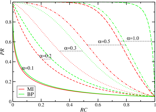
Figure 9: Increase in performance with $\alpha$, i.e. with the number of presented patterns.

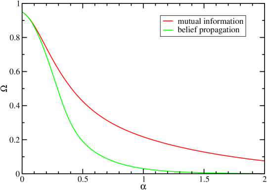
Figure 10: Prediction error as a function of the number $M=\alpha N$ of presented patterns, for both algorithms based on pairwise mutual information (red line) and belief propagation (green line, measured at constant dilution $n_{eff}=0.04$.

To complete our analysis, we have also included errors into the data generator, fixing all other parameters to $\alpha=0.5$ and $n_{eff}=0.04$. Other parameter values lead to qualitatively equivalent results. In Figs. 11 and 12 we have plotted the precision-vs.-recall curves and the prediction error for various values $\gamma$ of the noise strength. The predictive power of the algorithms obviously decreases with increasing noise level. Note, however, that even for $\gamma=k_{1}+4k_{2}$, where the statistical properties of the signal and of the noise are equivalent, a non-trivial prediction is possible.

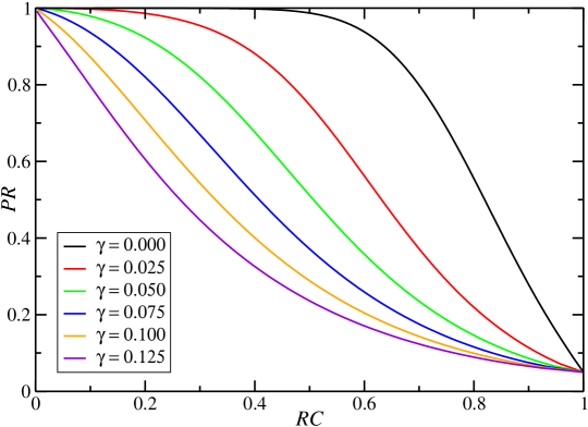
Figure 11: Precision versus recall of BP for various noise strengths $\gamma=0.0,\ 0.025,\ 0.05,\ 0.075,\ 0.1,\ 0.125$ (curves from right to left), ranging from no noise to equal signal and noise strengths.

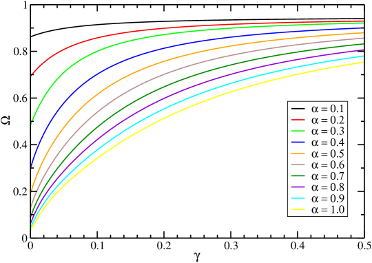
Figure 12: Prediction error of BP as a function of the noise strength $\gamma$, for various values of $\alpha$.

VI Conclusion and outlook

In this paper, we have analysed the performance of two approaches to the identification of gene-regulatory interactions. Whereas the first method is based on a ranking of all gene pairs according to the measured correlations between their expression levels, the second method tries to include collective effects of activators and repressors coming from the joint action of multiple regulators. This second method, developed by the same authors in an earlier publication, uses message-passing techniques (belief propagation) which can be understood as an algorithmic reinterpretation of the cavity method in spin-glass physics.

Using a simple data generator, we achieved a theoretical analysis of the algorithmic performance. In the simpler case of pairwise correlations, this analysis is based on a straight-forward application of the central limit theorem. The more involved case of the second algorithm requires the use of other spin-glass techniques, more precisely of the replica method in order to perform a generalised Gardner calculation in the space of all candidate gene networks. We found that algorithms taking into account collective effects beyond pair-correlations work better. The intuitive reason for this finding is that the best joint prediction is not necessarily done by the set of the best individual predictors. These results are true even if the data generator is more complex than the inference algorithm. We tested explicitly the cases of heterogeneous regulation strengths and noisy data.

There are some interesting directions to be followed. First of all, these algorithms are designed to be applied to real biological data. As already seen in BP-infer , also BP can be used to extract sparse and predictive information from gene-expression data. Still there is space for substantial improvements by integration of biological knowledge which goes beyond a simple diluting field. One possibility is, e.g., the integration of sequence information on putative transcription factor binding sites via inhomogeneous diluting fields.

One drawback in both the considered data generator and the derivation of the BP algorithm is that we neglected correlations between inputs. These correlations exist, however, in biological data, since also transcription factors may be coregulated. An interesting approach in this direction was recently presented by Kabashima Ka , and can be extended to our model. It would be interesting to see under which conditions correlations really change the behaviour of the algorithms.

A last point is the application of the algorithm to other problems. In fact it gives more generally a sparse Bayesian classifier. Bioinformatical applications of such classifiers goes far beyond the inference of gene networks. One example we are currently analysing is the classification of expression patterns of cancer tissues according to their diagnosis (cancer vs. healthy tissues, different cancer subtypes), and the detection of predictive but sparse gene signatures for the different diagnoses UdKa ; FraTrig .

Acknowledgment: We are grateful to Yoshiyuki Kabashima, Michele Leone and Francesca Tria for interesting and helpful discussions.

References

- (1) B. Alberts, A. Johnson, J. Lewis, M. Raff, D. Bray, K. Hopkin, K. Roberts, and P. Walter, Essential Cell Biology (Garland Science, New York 2003)
- (2) S.S. Shen-Orr, R. Milo, Sh. Mangan, and U. Alon, Nat. Gen. 31, 64 (2002).
- (3) N. Guelzim, S. Bottani, P. Bourgine, and F. Kepes, Nat. Gen. 31, 60 (2002).
- (4) R. Milo, S.S. Shen-Orr, S. Itzkovitz, N. Kashtan, D. Chklovskii, and U. Alon, Science 25 824 (2002).
- (5) H. Bolouri and E. Davidson, Dev. Biol. 246, 2 (2002); E. Davidson et al., Science 295, 1669 (2002).
- (6) R. Albert and H.G. Othmer, Journal of Theoretical Biology 223, 1-18 (2003).
- (7) A.J. Butte and I.S. Kohane, in N. Lorenzi (ed.) Fall Symposium, American Medical Informatics Association (Hanley and Belfus, Washington DC, 1999).
- (8) A.J. Butte, P. Tamayo, D. Slonim, T.R. Golub, I.S. Kohane, Proc. Nat. Acad. Sci. 97, 12182 (2000).
- (9) A.A. Margolin, I. Nemenman, K. Basso, C. Wiggins, G. Stolovitzky, R. Dalla Favera and A. Califano, BMC Bioinformatics 7, S7 (2006).
- (10) K. Basso, A. Margolin, G. Stolovitzky, U. Klein, R. Dalla-Favera, and A. Califano, Nat Genet. 37, 382 (2005).
- (11) K. Murphy and S. Mian, Technical Report, University of California, Berkeley (1999).
- (12) N. Friedman, M. Linial, I. Nachman, and D. Pe’er, J. Comp. Biol. 7, 601 (2000).
- (13) Jing Yu, V.A. Smith, P.P. Wang, A.J. Hartemink, and E.D. Jarvis, Bioinformatics 20, 3594 (2004).
- (14) A.J. Hartemink, Nature 23, 554 (2005).
- (15) I. Shmulevich, E.R. Dougherty, and W. Zhang, Proc. of the IEEE, Vol. 90, No. 11, p. 1778 (2002).
- (16) R.F. Hashimoto, S. Kim, I. Shmulevich, W. Zhang, M. L. Bittner, E.R. Dougherty, Bioinformatics 20, 1241 (2004).
- (17) M. Baillet-Bechet, A. Braunstein, A. Pagnani, M. Weigt, and R. Zecchina, preprint (2008).
- (18) A. Braunstein, A. Pagnani, M. Weigt, and R. Zecchina, J. Phys.: Conf. Ser. 95, 012016 (2008).
- (19) N. Buchler, U. Gerland and T. Hwa, Proc. Nat, Acad. Sci. 100, 5136 (2003).
- (20) J. Hertz, A. Krogh, and R. G. Palmer, Introduction to the Theory of Neural Computation, (Addison-Wesley, Redwood CA 1991).
- (21) A. Engel and C. van den Broeck, Statistical mechanics of learning (Cambridge University Press, New York 2001).
- (22) E. Gardner, Europhys. Lett. 4, 481 (1987); J. Phys. A: Math. Gen. 21, 257 (1988).
- (23) R. Tibshirany, J. R. Statist. Soc. B 58, 267 (1996).
- (24) P. Ravikumar, M.J. Wainwright, J.D. Lafferty, Technical Report, Dep. of Statistics, UC Berkeley (2008)
- (25) O. Banerjee, L. El Ghaoui, A. d’Aspremont, and G. Natsoulis. ACM International Conference Proceeding Series Vol. 148 p. 89 (Pittsburgh Pennsylvania, 2006).
- (26) S.I. Lee, V. Ganapathi, and D. Koller, in Advances in Neural Information Processing Systems (NIPS 2006), ed. B. Schölkopf, J. Platt, T. Hofmann (MIT Press, 2007)
- (27) M. Schmidt, A. Niculescu-Mizil, and K.Murphy, in Proc. 22nd AAAI Conf. on Artificial Intelligence (American Association of Artificial Intelligence, 2007)
- (28) N. Meinshausen and P. Buehlmann, Ann. Stat. 34, 1436 (2006).
- (29) Y. Kabashima, J. Phys. A 36, 11111 (2003).
- (30) S. Uda and Y. Kabashima, J. Phys. Soc. Jpn. 74, 2233 (2005).
- (31) A. Braunstein and R. Zecchina, Phys. Rev. Lett. 96, 030201 (2006).
- (32) Y. Kabashima, J. Phys.: Conf. Ser. 95, 012001 (2008).
- (33) F. Tria, A. Pagnani, and M. Weigt, submitted (2008).