SCALING OF THE DIFFUSION COEFFICIENT ON THE NORMAL FORM REMAINDER IN DOUBLY-RESONANT DOMAINS

Abstract

An outline of theoretical estimates is given regarding the dependence of the value of the diffusion coefficient $D$ on the size $R$ of the remainder of the normal form in doubly or simply resonant domains of the action space of 3dof Hamiltonian systems.

C. EFTHYMIOPOULOS¹

¹Research Center for Astronomy, Academy of Athens, Soranou Efessiou 4, 115 27 Athens, Greece

E--mail cefthim@academyofathens.gr

1 INTRODUCTION

In the works of Froeschlé et al. (2000, 2005, 2006), Lega et al. (2003), and Guzzo et al. (2005) precise numerical estimates were given of the critical threshold (in terms of a small parameter $\epsilon$) at which one has the onset of the so-called ‘Nekhoroshev regime’ (Nekhoroshev 1977, Benettin et al. 1985, Lochak 1992, Pöshel 1993) in conservative systems of three degrees of freedom. In the same works the local speed of Arnold diffusion, as well as the exponents appearing in the associated laws of the Nekhoroshev theory, were estimated. Other studies by the same group are Guzzo et al. (2006, effects of non-convexity) and Todorovic et al.(2008, diffusion in ‘a priori unstable’ systems). Earlier studies are: Kaneko and Konishi (1989), Wood et al. (1990), Dumas and Laskar (1993), Laskar (1993), Skokos et al. (1997), Giordano and Cincotta (2004).

In a recent study (Efthymiopoulos 2008), we used a computer program to carry on Hamiltonian normalization up to a sufficiently high order, and found that in a case of simple resonance the size $R$ of the optimal remainder of the normalized Hamiltonian (which turned to be exponentially small in $1/\epsilon^{a}$, $a\simeq 0.25$) scales with the diffusion coefficient of numerical experiments as $D\propto R^{3}$. This scaling law was presented as an empirical fact, no theory behind being suggested. Furthermore, no investigation was made of what happens in cases of double resonance. The above two questions are briefly addressed in the sequel. In particular, theoretical estimates of the scaling law $D(R)$ are outlined, first in the case of double and then of simple resonances. Details are deferred to a paper under preparation.

2 OUTLINE OF ESTIMATES ON THE LAW $D(R)$

We shall refer to Hamiltonian systems of three degrees of freedom

$$H(I,\phi)=H_{0}(I)+\epsilon H_{1}(I,\phi)$$ (1)

where $I\equiv(I_{1},I_{2},I_{3})$, $\phi\equiv(\phi_{1},\phi_{2},\phi_{2})$, $H_{0}$ satisfies appropriate non-degeneracy and convexity conditions, and $H$ is analytic in a complexified domain of the actions and the angles. The frequencies are $\omega(I)=\nabla_{I}H_{0}(I)$. Owing to the analyticity condition, the Fourier series $H_{1}=\sum_{k}h_{k}(I)\exp(ik\cdot\phi)$ yields coefficients $h_{k}$ decaying exponentially with the modulus of the vector $k$, namely the bound $|h_{k}(I)|<A\exp(-|k|\sigma)$ holds with $|k|=|k_{1}|+|k_{2}|+|k_{3}|$ and $A,\sigma$ positive constants. Consider an open domain ${\cal W}_{I_{*},D}$ in the action space, of size $D$, centered around some central value $I_{*}$. Expanding $H_{0}$ around $I_{*}$ leads to

$$H_{0}=H_{0*}+\omega_{*}\cdot J+{1\over 2}M_{ij*}J_{i}J_{j}+\ldots$$ (2)

where $J=I-I_{*}$, $\omega_{*}=\nabla_{I}H_{0}(i_{*})$, $M_{ij*}$ are the entries of the Hessian matrix of $H_{0}$ at $I_{*}$ (which satisfy restrictions imposed by the convexity condition). Assuming some truncation order $K_{c}$ in Fourier space, we consider the case in which there are two linearly independent integer vectors $k^{(1)}$, $k^{(2)}$ both satisfying the conditions $|k^{(j)}|<K_{c}$, $k^{(j)}\cdot\omega_{*}=0$, $j=1,2$. A normalization of the Hamiltonian (1) valid in ${\cal W}_{D,I_{*}}$ results in that all the resonant trigonometric terms, of the form $\exp(i((q_{1}k^{(1)}+q_{2}k^{(2)})\cdot\phi)$, with $q_{1},q_{2}$ integers, $|q_{1}k^{(1)}+q_{2}k^{(2)})|<K_{c}$, survive in the normal form. Choosing a vector m satisfying $m\cdot k^{(j)}=0,j=1,2$, and setting $J_{i}=k_{i}^{(1)}I_{R}^{(1)}+k_{i}^{(2)}I_{R}^{(2)}+m_{i}I_{F}$, $\phi_{R}^{(j)}=k^{(j)}\cdot\phi$, $\phi_{F}=m\cdot\phi$, $i=1,2,3$, $j=1,2$, the normalized Hamiltonian takes the form (in new canonical variables)

$$H_{norm}=Z_{R}\left(I_{R}^{(1)},I_{R}^{(2)},I_{F},\phi_{R}^{(1)},\phi_{R}^{(2)}\right)+R\left(I_{R}^{(1)},I_{R}^{(2)},I_{F},\phi_{R}^{(1)},\phi_{R}^{(2)},\phi_{F}\right)~{}.$$ (3)

Two facts are relevant about (3): i) the angle $\phi_{F}$ is ignorable in the normal form $Z_{R}$. Therefore $I_{F}$ is an integral of the Hamiltonian flow under $Z_{R}$ alone. It follows that, for different label values of $I_{F}$, $Z_{R}$ alone defines the dynamics of a system of two degrees of freedom. ii) The (optimal) remainder is exponentially small $R=O(\exp(-1/\epsilon))$, thus it only slightly alters the dynamics due to the normal form.

Now, the convexity condition ensures that there is a linear canonical transformation $(J_{R}^{(1)},J_{R}^{(2)},\phi_{R}^{(1)},\phi_{R}^{(2)})$ $\rightarrow$ $(J^{\prime}_{1},J^{\prime}_{2},\phi^{\prime}_{1},\phi^{\prime}_{2})$ such that in the new variables the Hamiltonian reads $Z_{R}={1\over 2}\left[{\cal A}_{1}(J_{1}^{\prime}-c_{F,1})^{2}+{\cal A}_{2}(J_{2}^{\prime}-c_{F_{2}})^{2}\right]+\ldots+\epsilon\sum_{n}C_{n}(J_{1}^{\prime},J_{2}^{\prime};\epsilon,I_{F})$ $\times\exp(in\cdot\phi^{\prime})$, the constants ${\cal A}_{1}$, ${\cal A}_{2}$ being positive and depending on $M_{ij*}$, and $c_{F,1},c_{F,2}$ depending on $M_{ij*}$ as well as on the value of the integral $I_{F}$. Apart from trivial modifications, the dynamics of $Z_{R}$ is then the same as under the simplified model

$$Z_{R}={1\over 2}\left[(J_{1}^{\prime}-c_{F,1})^{2}+(J_{2}^{\prime}-c_{F_{2}})^{2}\right]+\epsilon\sum_{n}C_{n}(J_{1}^{\prime},J_{2}^{\prime};\epsilon,I_{F})\exp(in\cdot\phi^{\prime})$$ (4)

which we now consider in some detail.

For any fixed value of the angles $(\phi_{1}^{\prime},\phi_{2}^{\prime})$, the constant energy condition $Z_{R}=E$ implies that the actions $J_{1}^{\prime},J_{2}^{\prime}$ lie on a circle of radius $\sqrt{2E}$ centered at $(J_{1}^{\prime},J_{2}^{\prime})=(c_{F,1},c_{F_{2}})$. This is shown schematically in Figure 1. As the angles $\phi^{\prime}$ change value, the trigonometric terms in (4) can only induce a $O(\epsilon)$ change in the radius of the circle, which we shall temporarily ignore. On the other hand, the lines $m_{1}^{\prime}J_{1}^{\prime}+m_{2}^{\prime}J_{2}^{\prime}=0,~{}~{}~{}m^{\prime}\cdot n=0$, where $n$ is the integer vector of any trigonometric term appearing in (4), define the 1D resonant manifolds of the Hamiltonian (4) in the reduced 2D action space. By construction, the Hamiltonian (4) contains only a finite number of harmonics with coefficients $C_{n}$ scaling as $|C_{n}|\sim\epsilon\exp(-\sigma|n|)$. It follows that there is a finite set of resonant lines in Fig.1, all passing from the center of the circles of constant energy. Three such lines are shown schematically (black solid). The pairs of dashed lines defining the boundaries of the zones around the resonant lines correspond to the limits of the separatrix width of each resonance, which is of the order

$$\Delta J_{n}\sim\left(\epsilon\exp(-\sigma|n|)\right)^{1/2}~{}~{}.$$ (5)

The smaller the value of $|n|$ the larger the width of the resonance. Thus, in Fig.1 we have $|n_{1}|<|n_{2}|<|n_{3}|$.

The resonances are well separated if the energy $E$ is large enough (big circle in Fig.1, at $E=E_{1}$). Since the entire set of resonances cover an $O(\epsilon^{1/2})$ length of an arc on a circle of constant energies, significant resonance overlap occurs if $E=O(\epsilon)$ or smaller (small circle for $E=E_{2}$ in Fig.1).

So far we have neglected the effect of the remainder. This is manifested by causing a slow drift of the normal form energy value $E_{NF}$ of the orbits run under the full Hamiltonian, compensating the drift in the remainder value so that the total energy $E=E_{NR}+R$ be a constant. In Fig.1 this drift is shown by curly curves. An orbit found at a given time near the separatrix of, say, resonance 1, with $E_{NF}=E_{1}$, has a certain probability to slowly drift in the action space outwards ($E_{NF}$ increases) or inwards ($E_{NF}$ decreases). Assume the latter case. Then, after a long time the orbit will be found touching the inner circle $E=E_{2}$, where all resonances overlap. If, still later, the drift is reversed (again with a certain probability), $E_{NF}$ will increase and the orbit will return to the circle $E_{NF}=E_{1}$, but this time lying, in general, on the separatrix layer of a different resonance, say resonance 2.

This qualitative picture of the diffusion in resonance junctions should, of course, be substantiated by calculating the invariant manifolds of the 2D tori lying at the borders of the resonances of the full Hamiltonian system. If there are heteroclinic intersections between these manifolds, an orbit started on one manifold is guaranteed to undergo the type of drift motion described above. However, verifying this fact numerically poses a formidable task, equivalent to probing the very mechanism of Arnold diffusion. This restriction notwithstanding, we proceed in a plausible quantitative estimate of the speed of the diffusion on the basis of numerical experiments having observed, instead, the drift in the action space directly (as e.g. in Lega et al. 2003). The indication from such experiments is that the drift in the action space can be modeled, at least locally, like a normal diffusion process. Assuming this true, one may ask how long it will take for, say, the curly itinerary of Fig.1 to be realized. Attributing the drift to the remainder, the per step change of the $E_{NF}$ value of an orbit crossing the junction is $dE\sim R$. By Fick’s law, one then has after $N$ steps a total change $\Delta E_{NF}\sim N^{1/2}dE=N^{1/2}R$. By (5) the radius of the outermost circle touching the junction’s limits is $\Delta J=O(\epsilon^{1/2})$, implying that the total drift in the value of $E_{NF}$ is $\Delta E_{NF}=O(\epsilon)$. Putting these relations together one then finds for the diffusion coefficient $D\sim\Delta J^{2}/N$ the relation $D\sim\epsilon^{-1}R^{2}$. Note that, since $R=O(\exp(-1/\epsilon))$ one has, by de l’Hopital’s rule that $D\sim R^{2}\rightarrow 0$ in the limit $\epsilon\rightarrow 0$.

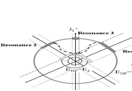
Figure 1: The circles of constant normal form energy $E_{NF}$ and the drift of the orbits in resonance junctions (see text)

A similar calculation can be made in the case of simple resonances, if we take into account that the simply-resonant domains are, in fact, composed also by sub-domains ${\cal W}_{D,I_{*}}$ crossed by multiple resonances, the difference from doubly resonant domains being essentially that only one of these resonances satisfies $|k^{(1)}|<K_{c}$, while all the others satisfy $|k^{(2)}|\geq K_{c}$. Since all apart one resonances are contained in the remainder function, it follows that the total travel to cross a resonant junction in the action space is now of order $R^{1/2}$ (instead of $\epsilon^{1/2}$ in double resonances). Setting $\Delta J^{2}\sim R$ we then readily find $D\sim\epsilon^{-2}R^{3}$.

In conclusion, we predict that in systems like (1) the local value of the diffusion coefficient $D$ scales with the size of the optimal remainder function $R$ of the local normal form as a power law $D\sim R^{b}$, the estimate $b\approx 2$ holding close to doubly-resonant domains and $b\approx 3$ close to simply-resonant domains. It would be of interest to check these theoretical estimates against detailed numerical experiments.

References

Arnold, V.I., 1964: Sov. Math. Dokl. 6, 581.

Benettin, G., Galgani, L., and Giorgilli, A.: 1985, Cel. Mech. 37, 1.

Dumas, H.S., and Laskar, J.: 1993, Phys. Rev. Lett. 70, 2975. Froeschlé, C., Guzzo, M., and Lega, E.: 2000, Science 289 (5487), 2108.

Efthymiopoulos, C: 2008, Cel. Mech. Dyn. Astron., 102, 49.

Froeschlé, C., Guzzo, M., and Lega, E.: 2000, Science 289 (5487), 2108.

Froeschlé, C., Guzzo, M., and Lega, E.: 2005, Cel. Mech. Dyn. Astron. 92, 243.

Froeschlé, C., Lega, E., and Guzzo, M.: 2006, Cel. Mech. Dyn. Astron. 95, 141.

Giordano, C.M., and Cincotta, P.M.: 2004, Astron. Astrophys. 423, 745.

Guzzo, M., Lega, E., and Froeschlé, C.: 2005, Dis. Con. Dyn. Sys. B 5, 687.

Guzzo, M., Lega, E., and Froeschlé, C.: 2006, Nonlinearity, 19, 1049.

Kaneko, K., and Konishi, T.: 1989, Phys. Rev. A 40, 6130.

Laskar, J.: 1993, Physica D67, 257.

Lega, E., Guzzo, M., and Froeschlé, C.: 2003, Physica D 182, 179.

Lochak, P.: 1992, Russ. Math. Surv. 47, 57.

Nekhoroshev, N.N.: 1977, Russ. Math. Surv. 32(6), 1.

Pöshel, J.: 1993, Math. Z. 213, 187.

Skokos, C., Contopoulos, G., and Polymilis, C.: 1997, Cel. Mech. Dyn. Astr. 65, 223.

Todorovic, N., Lega, E., and Froeschlé, C.: 2008, Cel. Mech. Dyn. Astr., 19, 1049.

Wood, B.P., Lichtenberg, A.J., and Lieberman, M.A.: 1990,Phys. Rev. A 42, 5885.