White dwarfs in the Capodimonte deep field

Abstract

Aims. In this article we describe the search for white dwarfs (WDs) in the multi-band photometric data of the Capodimonte deep field survey.

Methods. The WD candidates were selected through the $V-R_{C}$ vs $B-V$ color-color diagram. For two bright objects, the WD nature has been confirmed spectroscopically, and the atmospheric parameters (T_eff  and $\log g$) have been determined. We have computed synthetic stellar population models for the observed field and the expected number of white dwarfs agrees with the observations. The possible contamination by turn-off and horizontal branch halo stars has been estimated. The quasar (QSO) contamination has been determined by comparing the number of WD candidates in different color bins with state-of-the-art models and previous observations.

Results. The WD space density is measured at different distances from the Sun. The total contamination (non-degenerate stars + QSOs) in our sample is estimated to be around 30%. This work should be considered a small experiment in view of more ambitious projects to be performed in the coming years in larger survey contexts.

1 Introduction

The intrinsic faintness of white dwarfs (WDs) means that they are only seen at small distances from the Sun and that their statistical properties are still not well known. A complete sample of white dwarfs only exists in a small volume with a radius of 13 pc. Based on this sample of 43 stars, and adding another 79 objects with known distances all within 20 pc from the Sun, Holberg et al. (holberg08 (2008)) obtained a WD local space density of $(4.8\pm 0.5)\times 10^{-3}$ pc^-3.

Statistical studies of white dwarfs have been increasing in the past years, thanks to the results of recent and/or ongoing surveys, in particular the Sloan Digital Sky Survey (SDSS, Eisenstein et al. eisenstein06 (2006)), which has roughly doubled the number of spectroscopically confirmed white dwarfs, with about 6,000 new discoveries, allowing detailed studies of the mass distribution (Kepler et al. 2007) and the mass and luminosity function (De Gennaro et al. 2008 and references therein). However, the completeness limit of the SDSS photometric data, around g$\approx$19.5 (De Gennaro et al. 2008), is not deep enough to study the WD distribution of these stars across the galactic disk, and their scale height, in particular for the coolest objects. Deeper samples exist, for example the WD candidates identified in the Canada-France-Hawaii Telescope Legacy Survey (CFHTLS, Limboz et al. 2007), even though they are generally limited to small areas (3.6 square degrees for the CFHTLS WDs). Moreover, color selection alone is not enough to identify cool white dwarfs. For white dwarfs cooler than about 8,000 K, astrometry is essential when spectroscopic data are not available and the reduced proper motion diagram (Luyten 1918) is the best way to separate these objects from metal-weak, high-velocity, main-sequence Population II subdwarfs (Kilic et al. 2006).

Of particular interest are the so-called ultra-cool white dwarfs (T_eff$\stackrel{{\scriptstyle{\displaystyle<}}}{{\sim}}$4,000 K), very old objects that contain precious information on the primordial epoch of our galaxy. These objects fall near the deep minimum of the WD luminosity function, at L/L${}_{\odot}\simeq-4.5$, caused by the finite age of the galactic disk. Measuring the position of this minimum, we can measure the age of the galactic disk itself (D’Antona & Mazzitelli 1978, Harris et al. 2006 and references therein). Presently, the number of known ultra-cool WDs is about 20 (Harris et al. 2008) and most of them were discovered in the Sloan Digital Sky Survey.

For the future, one of the most ambitious projects that study the WD populations is the ESA Gaia astrometric space mission, which will be able to discover about 400,000 white dwarfs with a detection rate close to 100% up to 100 pc (Jordan 2007).

In this article we describe the search for white dwarfs in the multi-color photometric data of the Capodimonte deep field survey. In sect. 2 we present the selection criteria of our sample, based on morphological classification of point sources and colors. In sect. 3 we describe the spectroscopic results on three bright targets. In sect. 4 synthetic stellar population models are computed and the expected number of white dwarfs is compared with our sample. Contamination from turn-off and horizontal branch halo stars is estimated and discussed. QSO contamination is considered in sect. 5, where our results are discussed and compared with previous findings.

2 Photometry: selecting WD candidates

The “Osservatorio Astronomico di Capodimonte” Deep Field (OACDF, Alcalá et al. 2004) is a multi-band ($B,V,R_{C}$  plus shallow $I_{C}$) photometric survey covering 0.5 square degrees at high galactic latitude (RA₂₀₀₀$\simeq$12:25, DEC₂₀₀₀$\simeq$–12:49 or $l\simeq$293.0, $b\simeq$49.56 in galactic coordinates), performed using the Wide Field Imager (WFI) attached to the ESO 2.2 m telescope at La Silla observatory. The 5 $\sigma$ limiting magnitudes are: B_AB=25.3, V_AB=24.8 and R_AB=25.1. Typical errors (including source extraction, zero-points and extinction terms) at magnitude 20 (23) are 0.06 (0.10) mag in the $B$ band and 0.05 (0.08) mag in $V$ and $R_{C}$.

2.1 Extra-galactic extended contaminants

From the original catalogs of the OACDF survey, we optimized the selection criteria to isolate point source objects from extended ones, using the flux radius parameter from SExtractor (Bertin & Arnouts 1996). Flux radius is the aperture radius in pixels (1 pix = 0.238 arcsec for WFI) where a defined fraction of the light (50% in our case) is collected.

Fig. 1 represents the flux radius versus magnitude, where the stellar branch can be easily identified. The six panels refer to the $BVR_{C}$ bands in two adjacent WFI fields (OACDF2 and OACDF4). We can see that the contamination from extended objects starts typically near magnitude 21-22, depending on the photometric band considered, and becomes quite strong at magnitude $\sim$23 (or $\sim$24 in the $B$ band). The selected objects (black points) are those falling inside the boxes indicated in Fig. 1. This criterion must be valid for the three $BVR_{C}$ photometric bands simultaneously. In this way we can exclude most of the extra-galactic extended sources and saturated stars that lie in the left upper part of each box.

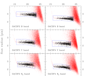
Figure 1: Selection of point sources objects from the OACDF catalogs. The polygons represent the regions where the point-like objects are concentrated (see the text for more details).

2.2 WD candidates from the color-color diagram

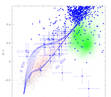
Figure 2: Color-color plane of the OACDF point source objects (blue dots) compared with Bergeron’s theoretical WD tracks with $\log g=7.0,7.5,8.0,8.5,9.0,9.5$ (H WDs) or $\log g=7.0,7.5,8.0,8.5,9.0$ (He WDs) from http://www.astro.umontreal.ca/ bergeron/CoolingModels/ (see Holberg & Bergeron 2006 and references therein for more details). The objects with error bars represent the WD candidates with $B-V<0.35$. The three circled points represent the WD candidates for which spectroscopy was performed (see Section 3). Since galactic reddening is rather small (at most E$(B-V)=0.05$ and E$(V-R_{C})=0.03$ mag for the hotter objects, more distant from us and outside the disk), extinction is not considered in this plot. The green, red and black points represent, respectively, all the SDSS quasars, white dwarfs and hot subdwarfs (see the text for more details). Note that the black symbols of the hot subdwarfs are slightly larger in order to enhance these rare objects. On the top of the QSO cloud, near the upper right corner, the clump of OACDF red dwarfs is visible.

To select the white dwarf candidates, in Fig. 2 the position of the point-like sources in the ($V-R_{C}$, $B-V$) plane is compared with the theoretical WD tracks from Holberg & Bergeron (2006) and with the location of the SDSS quasars (Data Release 5, Schneider et al. 2007), white dwarfs and hot subdwarfs (Data Release 4, Eisenstein et al. 2006). The Sloan colors of the SDSS objects were converted to the Johnson-Cousin system using the color transformations of Jester et al. (2005). The small discrepancy between WD tracks and hot SDSS white dwarfs (the latter being $\sim$0.05 redder in $V-R_{C}$) is due to the fact that Jester’s equations are not optimized for very blue objects. We have verified that in a ($g-r$, $r-i$) plane, the agreement between WD tracks and hot SDSS white dwarfs is much better (Bergeron’s evolutionary tracks are available also in Sloan colors).

Considering only the hottest objects ($B-V<0.25$), there are 21 WD candidates whose location is compatible with H or He white dwarfs having an effective temperature higher than about 8,400 or 8,100 K respectively. Another $\sim$19 objects falling on the right side of the WD cooling tracks could be white dwarfs with a red companion. However, in this region contamination from quasi-stellar objects (QSOs) is very strong at $B-V$ $\stackrel{{\scriptstyle{\displaystyle>}}}{{\sim}}$ $0$ (see Fig.2), and therefore most of these objects must be QSOs. For three of them, having very blue colors ($B-V<-0.1$), we can exclude a QSO nature: these objects can be either white dwarfs or hot subdwarfs with a cool companion. We know that a significant fraction of hot subdwarfs ($\sim$50% or even more for subdwarf B stars, Morales Rueda et al. 2006) reside in binaries; however hot subdwarfs are much more rare than white dwarfs (see Fig.2 and caption). Therefore these 3 objects are included in our list of WD candidates. Extending our color limit to $B-V=0.35$ (corresponding to T_eff$\simeq$ 7,150 K for both H and He WDs), the total number of WD candidates increases by a factor of $\sim$2 but the selection becomes more difficult because in this region the WD cooling tracks are very close (almost inside) the QSO clump. At $B-V$ $\stackrel{{\scriptstyle{\displaystyle>}}}{{\sim}}$ $0.25$, also the contamination from OB stars (main sequence objects and horizontal branch stars) starts. As a general criterion we have considered as WD candidates the objects whose error bars intersect the WD cooling tracks, excluding the regions where the QSO density dominates. In this way we add 8 more WD candidates, bringing to 32 the total number of WD candidates with $B-V<0.35$.

At $B-V$ $\stackrel{{\scriptstyle{\displaystyle>}}}{{\sim}}$ $0.35$ - $0.40$, stellar contamination becomes important, in particular from halo objects (see section 4). In order to be identified, cool white dwarfs require astrometric data and the use of the reduced proper motion diagram. These objects are not considered in this article.

3 Spectroscopy of three bright WD candidates

Among the WD candidates, three bright stars, marked with a circle in Fig. 2, were selected to perform spectroscopic follow-up. The spectroscopic observations were carried out at La Silla observatory using EMMI at the NTT and EFOSC2 at the 3.6 m telescope, both with the MOS (Multi-object spectroscopy) configuration. In the case of EMMI, the grism number 5 was used, with a spectral coverage from 4000 to 6600 Å, and a resolution of 5 Å  FWHM (implying a resolving power R$\sim$1100 at central $\lambda$). In the case of the EFOSC2 instrument, the grism number 1 was used, covering the spectral range from 3200 to 9000 Å  with a resolution of 40 Å  FWHM (R$\sim$150 at central $\lambda$).

The data were reduced using the standard procedures within the ESO-MIDAS  reduction package. First the images were corrected for bias and flat field; then the spectra were extracted and wavelength calibrated using arc lamp observations; finally, they were flux-calibrated. From an inspection of the spectra, two objects with the unique presence of Balmer lines have been confirmed to be DA white dwarfs. Their flux calibrated spectra are shown in Fig. 3. The third object (which has the up-right position in Fig. 2) has colors compatible both with a 8,500 K WD and a A8 main sequence star (e.g. Kenyon & Hartmann 1995). However, its H$\beta$ and H$\gamma$ lines are narrower than typical WDs and therefore this star was identified as a A8 star. Its spectrum is shown in Catalán et al. (2007).

The effective temperature (T_eff) and surface gravity ($\log g$) of the two confirmed WDs have been obtained following the prescriptions described in Catalán et al. 2007. The method consists mainly in normalizing the spectra to the continuum and fitting the theoretical models of DA white dwarfs by D. Koester (private communication) to the observed Balmer lines using the package SPECFIT under IRAF . This package is based on $\chi^{2}$ minimization using the method of Levenberg-Marquardt (Press et al. 1992). The white dwarf models had been previously normalized to the continuum and convolved with a Gaussian instrumental profile with the proper FWHM in order to have the same resolution as the observed spectra. In Fig. 4 the fits of the white dwarf models (sharp lines) to the observed Balmer lines of the two confirmed white dwarfs are shown. In the case of OACDF122406.4-124855 the spectral range is from H$\beta$ to H$\epsilon$, while in the case of OACDF122429.3-131413 the spectral coverage is narrower, including H$\beta$ and H$\gamma$ only.

Table 1: Photometric and stellar parameters of the spectroscopically confirmed white dwarfs

Name	$V$	$B-V$	$V-R_{C}$	$V-I_{C}$	$T_{\rm eff}$ (K)	$\log g$ (cgs)	$M_{\star}$ ($M_{\odot})$	$t_{cool}$ (Gyr)	$d$ (pc)∗
OACDF122406.4-124855	19.44$\pm$0.03	–0.10$\pm$0.05	–0.02$\pm$0.04	0.61$\pm$0.06	32,400$\pm$1,300	8.40$\pm$0.90	0.88$\pm$0.34	$<$0.13	620$\pm$${}^{610}_{350}$
OACDF122429.3-131413	19.57$\pm$0.04	0.24$\pm$0.07	0.04$\pm$0.06	0.03$\pm$0.07	10,700$\pm$300	7.92$\pm$0.05	0.56$\pm$0.02	0.44$\pm$0.04	350$\pm$20

^∗ Taking into account galactic extinction the distances are reduced by 20-25 pc.

Figure 3: Flux calibrated spectra of the two confirmed white dwarfs.

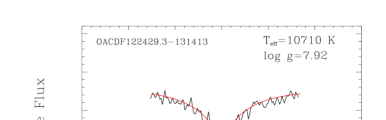
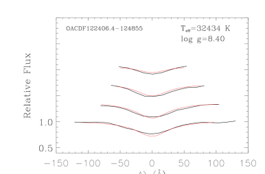
Figure 4: Model fits (sharp lines) to the individual Balmer line profiles of the two DA WDs detected in this survey. Lines range from H$\beta$ (bottom) to H$\epsilon$ (top) in the case of OACDF122406.4-124855 and from H$\beta$ (bottom) to H$\gamma$ (top) in the case of OACDF122429.3-131413. T_eff and $\log g$ from the best fit are indicated.

Once we have defined T_eff  and $\log g$  for each star, we determine its mass (M_⋆) and its cooling time (t_cool, time elapsed since the planetary nebula formation) using the cooling sequences of Salaris et al. (2000). Moreover, comparing the apparent V magnitude with the absolute magnitude expected from Bergeron’s models, we obtain an estimate of the distance. Our results are shown in Table 2.

The large errors associated with the hotter white dwarf are due to the low resolution of the spectrum, implying poor Balmer lines fitting. The formal error of 1,300 K in T_eff  is probably underestimated and the $B-V$ index would suggest a lower effective temperature near 23,000-24,000 K (considering a single WD). Even though the location of this object in Fig. 2 is compatible with a DB white dwarf, its spectrum does not show any He line, confirming its DA nature. The $V-R_{C}$ excess is likely due to a cooler companion, as confirmed by the high value of $V-I_{C}$ (see Table 1).

4 Comparing the WD candidates with synthetic stellar populations

Taking advantage of the stellar evolution theory and galactic structure, synthetic color-magnitude diagrams (CMDs) can be very useful to disentangle the stellar counts. Examples of this kind of analysis can be found in Bahcall & Soneira (BS (1984)), Castellani et al. (cast02 (2002)), Robin et al. (robin03 (2003)), Girardi et al. (girardi (2005)). Here we use the galactic model described in Cignoni et al. (cig08 (2008)).

Basically, field stars are not randomly distributed along the line of sight, but they are clumped according to the major galactic components (thin disk, thick disk, halo). Star count models exploit this point: although the distances are unknown, some assumptions can be made on the underlying spatial distributions. The following step is to convolve the spatial distribution with the underlying stellar populations. Once the number of synthetic stars for each galactic population at each distance from the Sun is computed, masses and ages are extracted populating specific initial mass functions (IMFs) and star formation rates (SFRs). Next, absolute magnitudes and colors are obtained by interpolating stellar tracks, whose metallicity is fixed by the assumed age-metallicity relation. Finally, reddening and photometric errors are applied to the synthetic photometry.

When a synthetic CMD is ready for a specific observed field (and scattered as a result of the photometric errors), it is straightforward to determine CMD regions where the white dwarfs are distinguishable from normal stars. In practice, depending on galactic latitude and WD colors, a galactic model is used to estimate the probability of contamination by: 1) halo turn-off stars; 2) halo blue Horizontal Branch (HB) stars; 3) massive thin disk stars in main sequence (which outnumber the WDs and have similar colors). Moreover it is possible to estimate the number of expected white dwarfs and distinguish thin disk white dwarfs from thick disk and halo WDs.

In our model the Galaxy is described by the following ingredients:

• Spatial distributions: The simulated Galaxy includes three main structures, namely the thin disk, the thick disk and the halo. The thin disk and the thick disk density laws are modeled by a double exponential (Reid & Majewski 1993): the main parameters governing these profiles are the scale length (fixed at 3500 pc for both populations) and the scale height (1 kpc for the thick disk, 250-300 pc for the thin disk). The halo follows a power law decay with exponent 3 (see Cignoni et al. cig07 (2007)) and an axis ratio of 0.8 (Gould et al. gould98 (1998)). A local spatial density of 0.11 stars $\mathrm{pc^{-3}}$ (Reid, Gizis & Hawley 2002) is adopted for the thin disk, whereas thick disk and halo normalizations are respectively 1/20 (Robin et al. robin96 (1996)) and 1/850 relative to the thin disk (Minezaki et al. minezaki98 (1998), Morrison et al. morrison (1993));

• Stellar tracks: For masses above $0.6\,M_{\odot}$, our code makes use of the Pisa stellar tracks (Cariulo et al. car (2004)), while, for the low mass range, colors are empirically fit to the faint end of nearby stars (thin disk) and the faint end of the cluster 47-Tucanae (thick disk). For the halo, the low mass range is treated using the theoretical calculations by Baraffe et al. (baraffe (1997)). To predict the CMD location of WDs we adopt the following ingredients: 1) a WD mass - progenitor mass relation (Weidemann et al. 2000); 2) WD cooling sequences (Salaris et al. salaris00 (2000)); 3) suitable model atmospheres (for $T_{eff}<4000\,\mathrm{K}$ the color relations are from Saumon & Jacobson saumon (1999), whereas for higher temperatures the calculations are from Bergeron, Wesemael & Beauchamp bergeron95 (1995)). The WD cooling age is given by the difference between the age of the star and the age of the WD progenitor at the end of the AGB. A further point of evolutionary significance concerns the CMD position of the synthetic HB stars: due to the unknown mechanism of mass loss during the red giant phase, halo stars which are predicted along the horizontal branch have been treated by assuming a Gaussian mass distribution centered on a mean mass $<M_{HB}>$, together with a mass dispersion $\sigma_{M}$ (see e.g. Castellani et al. cast05 (2005)). Masses and ages are then interpolated using HB stellar tracks.

• SFRs and chemical compositions: The thin disk SFR is assumed constant and only the old SFR cut-off is allowed to vary between 2 and 6 Gyr (see e.g. Cignoni et al. cig06 (2006)). The thin disk metallicity is fixed at $Z=0.02$. SFR and metallicity for halo and thick disk stars are derived from the comparison between synthetic and observed CMD. In the interval $19<V<23$ the CMD data shows a sharp cut-off in color ($0.38<B-V<0.45$). This feature can be reproduced using a galactic halo with metallicity $Z=0.0008$ (see also Cignoni et al. cig07 (2007)) and age 11-13 Gyr. Brighter than 19th magnitude, the observed turn-off moves to the red: although a solution in terms of age and metallicity cannot prove to be unique, a classical thick disk with $Z=0.006$ and a star formation activity older than 5 Gyr seems appropriate.

• IMFs: The IMF is a power law ($m^{-\alpha}$) for all populations: as a range of variation we assume the uncertainty on the exponent $\alpha$ as evaluated by Kroupa et al. kroupa (2001) ($\alpha=2.3\pm 0.3$).

Figure 5 shows the best synthetic diagram (only single stars, photometric errors are included) over-plotted onto the CMD data. The ingredients are indicated in Tab. 2.

Table 2: Ingredients for the galactic model. The IMFs are from Kroupa et al. kroupa (2001).

	Z	SFR(constant)	spatial parameters (H,L)
DISK	0.02	0.1-6 Gyr	H=250 pc, L=3500
THICK DISK	0.006	5-10 Gyr	H=1 Kpc, L=3500
HALO	0.0008	11-13 Gyr	$\rho\propto R_{Gal}^{\,-3}$

All stars bluer than the halo turn-off are compatible with thin disk white dwarfs. However, it is crucial to evaluate any source of contamination.

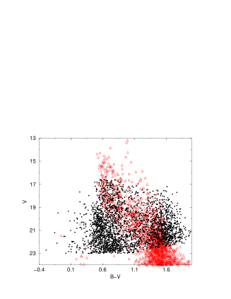
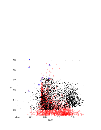
Figure 5: Color-magnitude diagram of the OACDF point source objects (black dots) compared with synthetic populations (triangles) of thin disk (upper panel), thick disk (middle panel) and halo (bottom panel) stars. Simulated halo HB stars (emphasized with big triangles) are computed using an HB mass dispersion $\sigma_{M}=0.005\,M_{\odot}$ and a mean mass $<M_{HB}>=0.68\,M_{\odot}$.

First, different halo models were considered: although the combination $Z=0.0008$ and age 11-13 Gyr reproduces well the turn-off region, to isolate a pure WD sample it is essential to explore also a metal poor halo (which may dominate sufficiently far out, see e.g. Carollo et al. carollo (2007)). In Figure 6 three halo models are compared with the observed color distribution (only stars with $V$ $<$ 23 are selected): interestingly, although the turn-off region is sensitive to the particular model, it is clear that a conservative cut at $B-V\sim 0.35$ significantly reduces the contamination of halo stars.

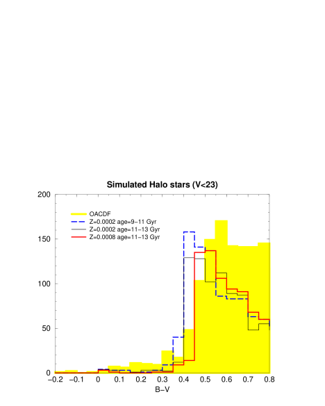
Figure 6: Comparison between synthetic (only halo stars) and observed color distribution ($V<23$). Different curves represent different halo models (HB stars follow the same prescription as in Fig. 5, $\sigma_{M}=0.005\,M_{\odot}$ and $<M_{HB}>=0.68\,M_{\odot}$). The yellow excess at $B-V$ $\stackrel{{\scriptstyle{\displaystyle<}}}{{\sim}}$ $0.35$ is largely due to the disk white dwarfs.

In particular, the turn-off stars, which make the major contribution, never exceed 13 objects, while only few HB stars are present. To evaluate the maximum HB contamination, the HB mass dispersion $\sigma_{M}$ is varied between 0.005 and $0.02\,M_{\odot}$, whereas the mean mass $<M_{HB}>$ is changed in the range $0.70-0.60\,M_{\odot}$. The simulations indicate that no more than 8 HB stars (where this number is obtained with a mean mass of $0.6\,M_{\odot}$, which is quite extreme) are expected in our field for $B-V<0.35$ and that they are all brighter than $V$$\sim$19. It is worth noting that about 25% of them are “lost” because they are brighter than the saturation limit ($V$$\sim$16 for the OACDF). So the maximum number of visible HB stars is about 6. In our list of OACDF WD candidates we have 2 stars brighter than $V$=19, one of them being indeed identified as a HB halo object (see sections 3 and 5 for more details).

As a final remark, we note that a few blue objects may be thick disk WDs: to test this circumstance, the model thick disk normalization is varied between 5% and 10% (which covers most of the current uncertainty). According to the simulations, the expected number of thick disk WDs with $B-V<0.35$ and $V<23$ is lower than 6-7 objects.

In summary, following our best simulations in Fig. 5, besides the thin disk WDs, the CMD region defined by $B-V<0.35$ and $16<V<23$ may host a few thick disk WDs ($\sim$3, maximum 6) and about 4 (up to 19 in the worst case) among turn-off and HB halo stars.

In order to provide a more quantitative analysis concerning the WD star counts, we have compared the observed number of WDs with the model predictions. Tab. 3 shows the predicted numbers assuming different IMFs, SFRs and thin disk scale heights. As expected, the WD counts increase adopting a shallower IMF, a younger SFR and a larger thin disk scale height.

Table 3: Mean number of predicted thin disk WDs with $B-V<0.35$ and $V<23$, for different combinations of IMF (exponent $\alpha$) and SFR (constant in the indicated interval). Results for a thin disk scale height H=250 pc and H=300 pc are shown.

		H=250 pc
$\alpha$	N( SFR 0-6 Gyr)	N(SFR 0-4 Gyr)	N(SFR 0-2 Gyr)
1.8	26	37	51
2.3	12	13	23
2.7	8	11	13
		H=300 pc
$\alpha$	N( SFR 0-6 Gyr)	N(SFR 0-4 Gyr)	N(SFR 0-2 Gyr)
1.8	40	53	77
2.3	22	23	31
2.7	13	15	19

From these simulations, if one assumes canonical values for the IMF exponent ($\alpha=2.3$) and the SFR (constant between 0 and 6 Gyr), we obtain 22 thin disk white dwarfs for a thin disk scale height H=300 pc. Adding also a few ($\sim$3) thick disk WDs, the total number of white dwarfs expected is not far from 32, as derived in section 2.2. Note that our list of WD candidates contains at least 4 (more likely 8-10, see Fig. 2) WDs in binaries, not included in our simulations.

5 Discussion

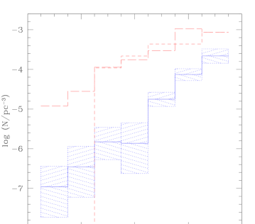
Figure 7: WD space density at various values of $B-V$. The continuous line is the space density obtained from our data with a V magnitude limit of 23 (shaded areas represent the errors). The long and short dashed lines represent, respectively, the WD space density expected from Begeron’s DA models with $\log g$=8.0 (Holberg & Bergeron 2006 and references therein), taking into account the mean duration of each evolutionary phase, and the WD local space density of Holberg et al. (2008) considering only objects with $B-V<0.35$. At $0.25<B-V<0.35$ the model density is normalized at the value of Holberg et al. (2008); note that their sample does not contain any hot white dwarf with $B-V<-0.15$. The great difference in number densities between our and Holberg’s data is due to the fact that we are sampling much more distant regions, in which the WD space density is much lower (see text for more details).

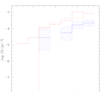
Figure 8: Same as Fig. 7 but with same volumes sampled in all the color bins. The continuous (blue) line is the space density within 897 pc from the Sun (shaded areas represent again the errors). In this plot the lower density of bluer objects is related only to their faster evolution.

In the previous section we have seen that the number of WD candidates that we have found is comparable with the number of disk white dwarfs predicted by synthetic color-magnitude diagrams (including a few thick disk WDs). In order to confirm the WD nature of these candidates, spectroscopy was performed for three of them: one is a non-degenerate star of spectral class A8. The color of this object ($B-V=0.24$), bluer than the halo turn-off, and its magnitude ($V=17.7$) suggest that it is a halo star on the horizontal branch (HB) at 25-30 kpc from us and $\sim$20 kpc from the galactic disk. This detection is consistent with the synthetic CMDs in Fig. 5 and confirms that stellar contamination is present in our sample.

In order to evaluate also the extra-galactic contamination (in particular from QSOs) and to compare the number of our WD candidates with previous results, we have calculated the space density in different $B-V$ color bins (Fig. 7). Considering that hotter and more luminous white dwarfs can be seen at larger distances, we have calculated the maximum radius at which a white dwarf can be seen with a magnitude limit $V=23$ for 7 different ranges of $B-V$ (absolute magnitudes are calculated using the Bergeron’s DA models, Holberg & Bergeron 2006 and references therein, assuming $\log g$=8.0). For each bin we have divided the number of WD candidates observed for the volume sampled. The WD density is then compared with what we expect from Bergeron’s DA models, considering the mean duration of the evolutionary phase corresponding to that particular color bin, and with the WD local space density obtained by Holberg et al. (2008). Note that what we can compare is only the slope of the density function. The number densities are necessarily different because Holberg et al. (2008) measure the local density (within 13 pc), whereas we are sampling more distant regions (see Table 4), up to the WD disk scale height and beyond, where the density of white dwarfs is much lower.

Fig. 7 shows that, when we move to hotter white dwarfs, the density decreases faster than Bergeron’s models and Holberg et al. (2008). This is not surprising because hot WDs are observed at larger distances, even well beyond the disk (at $B-V=-0.3$ the maximum distance is about 5,700 pc at $V=23$), where the space density is significantly lower. When we correct for this effect and recalculate the space densities considering same volumes in all the colors, the agreement with models and previous observations is much better (Fig. 8). This fact suggests that the residual contamination from QSOs in our sample is relatively small. Otherwise we would find a greater density in the redder color bin, where the frequency of QSOs is higher. Using small number statistics (Gehrels 1986), we can estimate a maximum QSO’s contamination of $\approx$50% in the reddest color bin.

Table 4: Number of WD candidates detected and space densities. The errors are calculated using small number statistics from Gehrels (1986).

	Vlim=21	Vlim=22	Vlim=23	d$<$357pc	d$<$566pc	d$<$897pc
				(z$<$273pc)	(z$<$434pc)	(z$<$687pc)
–0.35$<$B–V$<$–0.25	0	0	1	0	0	0
–0.25$<$B–V$<$–0.15	0	1	1	0	0	0
–0.15$<$B–V$<$–0.05	1	1	2	0	0	1
–0.05$<$B–V$<$ 0.05	0	1	1	0	0	0
0.05$<$B–V$<$ 0.15	2	4	8	0	1	2
0.15$<$B–V$<$ 0.25	5	6	11	3	5	6
0.25$<$B–V$<$ 0.35	5	6	8	5	6	8
TOT	13	19	32	8	12	17
space density (pc${}^{-3})$				(3.46$\pm$${}^{1.71}_{1.20}$)$\times$10-3	(1.31$\pm$${}^{0.50}_{0.37}$)$\times$10-3	(4.64$\pm$${}^{1.42}_{1.11}$)$\times$10-4

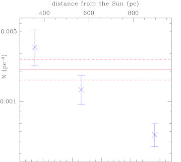
Figure 9: White dwarf space density at different distances from the galactic disk (z). The distribution is compatible with a scale height of about 200 pc. The horizontal line is the WD local space density (+ errors in dashed lines) of Holberg et al. (2008) considering only objects with $B-V<0.35$.

When we sum the space densities over all the color bins, we obtain the WD space density at various distances from the Sun or from the galactic disk (Fig. 9). The number of WD candidates in various colors and at various distances are given in Table 4. These densities do not include cool WDs with $B-V>0.35$ (or T_eff$\stackrel{{\scriptstyle{\displaystyle<}}}{{\sim}}$7150 K for DA WDs with $\log g$=8.0). In our smallest volume ($d<357$ pc) the WD space density, summing all the color bins, is $(3.5\pm^{1.7}_{1.2})\times 10^{-3}$ pc^-3 (see Table 4), 1.7 times greater than (but within the errors still compatible to) the local space density of Holberg et al. 2008 (they obtain $(2.1\pm 0.5)\times 10^{-3}$ pc^-3 considering only the WDs with $B-V$ between –0.35 and 0.35). If we consider a $B$ limiting magnitude of 22.5, the number of our WD candidates is reduced to 23$\pm$6 in 0.5 square degrees (or 46 per sq. degr.), which is 1.7$\pm$0.4 times higher than the sky surface density of 27 degr.^-2 obtained by Majewski & Siegel (2002) for $B$ $\stackrel{{\scriptstyle{\displaystyle<}}}{{\sim}}$ $22.5$ at the north galactic pole. The effective over-density is reduced from 1.7 to about 1.3 considering the different galactic latitude of the two fields (the OACDF is at $b\simeq 50$).

Conclusions:

• In the OACDF photometric survey we have identified 32 WD candidates. This number is in agreement (within the errors) with what we obtain from stellar synthetic populations in the same field.

• Our sample may be partially contaminated by blue stars and in particular by QSOs in the reddest color bins. As described in section 4, the stellar contamination from HB and turn-off halo stars can be estimated of the order of 10-15% (up to 60% in very unlikely circumstances). As seen in this section, the QSO contamination is estimated to be $\stackrel{{\scriptstyle{\displaystyle<}}}{{\sim}}$50% in the reddest color bin and almost zero elsewhere, giving a contribution of 10-15% to the total number of white dwarfs. Therefore we can consider a total contamination of the order of 30%.

• A selection effect is present for the white dwarfs with red companions. At $B-V$ $\stackrel{{\scriptstyle{\displaystyle>}}}{{\sim}}$ $0.05$ these objects are hardly identified because, in the color-color plane, they fall close to or inside the QSO’s region (Fig. 2).

• The WD sky surface density that we find is slightly higher than ($\sim$1.3 times) the value obtained by Majewski & Siegel (2002).

• The WD space density within $\sim$350 pc is 1.7 times greater than (but within the errors still compatible to) the measurements of Holberg et al. (2008) in the solar neighborhood.

The results presented in this article represent a small experiment in view of similar projects which are planned in the coming years in much wider ground-based survey contexts, such as KIDS/VIKING (see Arnaboldi et al. 2006), STREGA (Marconi et al. 2006) and the Alhambra Survey (Moles et al. 2008).

- (1) Alcalá, J.M., Pannella, M., Puddu, E. et al., 2004, A&A 428, 339
- (2) Arnaboldi, M., Neeser, M., Parker, L.C., et al., 2006, ESO Messenger, vol. 127, p. 28
- (3) Bahcall, J.N., Soneira, R.M., 1984, ApJS 55, 67
- (4) Baraffe, I., Chabrier, G., Allard, F., Hauschildt, P.H., 1997, A&A 327, 1054
- (5) Bergeron, P., Wesemael, F., Beauchamp, A., 1995, PASP 107, 1047
- (6) Bertin, E., Arnouts, S., 1996, A&AS 117, 393
- (7) Cariulo, P., Degl’Innocenti, S., Castellani, V., 2004, A&A 421, 1121
- (8) Carollo, D., Beers, T.C., Lee, Y.S., et al., 2007, Nature 450, 1020
- (9) Castellani, V., Cignoni, M., Degl’Innocenti, S., Petroni, S., Prada Moroni P.G., 2002, MNRAS, 334, 69
- (10) Castellani, V., Castellani, M., Cassisi, S., 2005, A&A 437, 1017
- (11) Catalán, S., Silvotti, R., Alcalá, J.M., Grado, A., Capaccioli, M., 2007, ASP Conf. Series 372, 135
- (12) Cignoni, M., Degl’Innocenti, S., Prada Moroni, P.G., Shore, S.N., 2006, A&A 459, 783
- (13) Cignoni, M., Ripepi, V., Marconi, M., Alcalá, J.M., Capaccioli, M., Pannella, M., Silvotti, R., 2007, A&A 463, 975
- (14) Cignoni, M., Tosi, M., Bragaglia, A., Kalirai, J.S., Davis, D.S., 2008, MNRAS 386, 2235
- (15) De Gennaro, S., von Hippel, T., Winget, D.E., et al., 2008, AJ 135, 1
- (16) D’Antona, F., Mazzitelli, I., 1978, A&A 66, 453
- (17) Eisenstein, D.J., Liebert, J., Harris, H.C., et al., 2006, ApJS 167, 40
- (18) Gehrels, N., 1986, ApJ 303, 336
- (19) Girardi, L., Groenewegen, M.A.T., Hatziminaoglou, E., da Costa, L., 2005, A&A 436, 895
- (20) Gould, A., Flynn, C., Bahcall, J.N., 1998, AJ 503, 798
- (21) Harris, H.C., Munn, J.A., Kilic, M., et al., 2006, AJ 131, 571
- (22) Harris, H.C., Gates, E., Gyuk, G., et al., 2008, ApJ 679, 697
- (23) Holberg, J.B., Sion, E.M., Oswalt, T., 2008, AJ 135, 1225
- (24) Holberg, J.B., Bergeron, P., 2006, AJ 132, 1221
- (25) Jordan S., 2007, ASP Conf. Series 372, 139
- (26) Jester, S., Schneider, D.P., Richards, G.T., et al., 2005, AJ 130, 873
- (27) Kenyon, S.J., Hartmann, L., 1995, ApJS 101, 117
- (28) Kepler, S.O., Kleinman, S.J., Nitta, A., et al., 2007, MNRAS 375, 1315
- (29) Kilic, M., Munn, J.A., Harris, H.C., et al., 2006, AJ 131, 582
- (30) Kroupa P., 2001, MNRAS 322, 231
- (31) Limboz, F., Karatas, Y., Kilic, M., Benoist, C., Alis, S., 2007, MNRAS 383, 957
- (32) Luyten, W.J., 1918, Lick Observatory Bulletin n.336, vol.10, p.135
- (33) Majewski, S.R., Siegel, M.H., 2002, ApJ 569, 432
- (34) Marconi, M., Musella, I., Ripepi, V., et al., 2006, MSAIS 9, 253
- (35) Minezaki, T., Cohen, M., Kobayashi, Y., Yoshii, Y., Peterson, B.A., 1998, AJ 115, 229
- (36) Moles, M., Benítez, N., Aguerri, J.A.L., et al., 2008, AJ 136, 1325
- (37) Morales-Rueda, L., Maxted, P.F.L., Marsh, T.R., Kilkenny, D., 2006, Baltic Astronomy vol.15, 187
- (38) Morrison, H.L., 1993, AJ 106, 578
- (39) Press, W.H., Flannery, B.P., Teukolsky, S.A., 1992, Numerical Recipes (Cambridge: Cambridge Univeristy Press)
- (40) Reid, N., Majewski, S.R., 1993, ApJ 409, 635
- (41) Reid, I.N., Gizis, J.E., Hawley, S.L., 2002, AJ 124, 2721
- (42) Robin, A.C., Haywood, M., Creze, M., Ojha, D.K., Bienayme, O., 1996, A&A 305, 125
- (43) Robin, A.C., Reylé, C., Derrière, S., Picaud, S., 2003, A&A 409, 523
- (44) Salaris, M., García Berro, E., Hernanz, M., Isern, J., Saumon, D., 2000, ApJ 544, 1036
- (45) Saumon, D., Jacobson, S.B., 1999, ApJ 511, L107
- (46) Schneider, D.P., Hall, P.B., Richards, G.T., et al., 2007, AJ 134, 102
- (47) Weidemann, V., 2000, A&A 363, 647