One-dimensional Ising ferromagnet frustrated by long-range interactions at finite temperatures

Abstract

We consider a one-dimensional lattice of Ising-type variables where the ferromagnetic exchange interaction $J$ between neighboring sites is frustrated by a long-ranged anti-ferromagnetic interaction of strength $g$ between the sites $i$ and $j$, decaying as $\mid i-j\mid^{-\alpha}$, with $\alpha>1$. For $\alpha$ smaller than a certain threshold $\alpha_{0}$, which is larger than 2 and depends on the ratio $J/g$, the ground state consists of an ordered sequence of segments with equal length and alternating magnetization. The width of the segments depends on both $\alpha$ and the ratio $J/g$. Our Monte Carlo study shows that the on-site magnetization vanishes at finite temperatures and finds no indication of any phase transition. Yet, the modulation present in the ground state is recovered at finite temperatures in the two-point correlation function, which oscillates in space with a characteristic spatial period: The latter depends on $\alpha$ and $J/g$ and decreases smoothly from the ground-state value as the temperature is increased. Such an oscillation of the correlation function is exponentially damped over a characteristic spatial scale, the correlation length, which asymptotically diverges roughly as the inverse of the temperature as $T=0$ is approached. This suggests that the long-range interaction causes the Ising chain to fall into a universality class consistent with an underlying continuous symmetry. The $e^{\Delta/T}$ temperature dependence of the correlation length and the uniform ferromagnetic ground state, characteristic of the $g=0$ discrete Ising symmetry, are recovered for $\alpha>\alpha_{0}$.

I Introduction

The competition between a short-ranged interaction favoring local order and a long-range interaction frustrating it on larger spatial scales is often used to explain pattern formation in chemistry, biology and physics Seul ; Muratov . The role of the long-range interaction is to avoid the global phase separation favored by the short-ranged interaction and promote a state of phase separation at mesoscopic or nano-scales. Thus, the long-range interaction is not, in general, a small perturbation Lieb ; Kiv1 ; Kiv2 ; Stariolo ; Nussinov_1 ; Nussinov_2 , but must be considered as precisely as possible. From a computational point of view, this means that the frustrating interaction has to be accounted for by involving all the lattice sites in the computation, which in turn limits the actual system size that can be handled in e.g. Monte Carlo (MC) simulations Debell ; Viot_1 ; Viot_2 ; Viot_3 ; Cannas ; Singer . Few exact results on multi-scale, multi-interaction Lieb ; Kiv1 systems are present – to our knowledge – in literature. For one-dimensional systems rigorous proof of absence of a phase transition in the pure long-range antiferromagnetic model has been obtained kerimov . Besides, rigorous results concerning the ground-state phase diagram can be found in Ref. Lieb, . Regarding two-dimensional lattice models with restricted spin orientation and dipole-dipole interaction competing with ferromagnetic nearest-neighbor exchange interaction, Giuliani et al. Lieb2 showed that the ground state is periodic striped, while a zero-temperature reorientation transition (from in-plane to out-of-plane magnetization) occurs at a given relative strength of the short- and long-range interaction when are both antiferromagnetic. Finally, a generalization of this periodic ground state in some continuum versions has been rigorously proved cheng ; Lieb3 ; muller .

In this paper, we perform MC simulations on a one-dimensional (1d) lattice with sites occupied by Ising-type classical variables assuming values $\sigma_{j}=\pm 1$. The nearest-neighbor sites interact by a short-ranged ferromagnetic interaction of strength $J$ which favors the same sign for two adjacent variables (in the language of magnetism the exchange interaction favors parallel alignment of neighboring spins). In addition, any two variables located at sites $i$ and $j$ interact by means of a long-range interaction of strength $g$ decaying according to a power law $\mid\!i\!-\!j\!\mid^{-\alpha}$ and favoring, instead, antiparallel alignment. In the present study, selected values of $\alpha>1$ and in the vicinity of 2 are investigated. This range turns out to be representative of the different physical regimes. We are aware of the apparently academic nature of $i.$) a one-dimensional model and of $ii.$) this choice of values for $\alpha$. In fact, point charges interact via the Coulomb interaction, which has $\alpha=1$, while the dipolar interaction between two localized magnetic moments has $\alpha=3$. On the other side, imposing a mono-dimensional modulation to two- or three-dimensional arrangements of charges and spins (a symmetry often realized in experiments Seul ; Muratov ; Ale ; Oliver1 ) produces an effective one-dimensional long-ranged interaction potential with an effective value of $\alpha$ which can differ from $1$ and $3$ respectively. As an example, elementary magnetic moments arranged into stripes and located on a two-dimensional array of sites interact with an effective, one-dimensional dipolar long-range interaction which, asymptotically, is proportional to $\mid\!i\!-\!j\mid^{-2}$ Ale . Accordingly, a systematic study for values of $\alpha$ in this range might reveal properties that can be used to explain physically relevant situations, such as those represented by the two-dimensional system of stripes quoted above or similar models of frustration discussed in connection with electronic phase separation Kiv2 . A 1d model has great computational advantages compared to its 2d and 3d counterparts, such as the possibility of simulating lattices of larger linear dimensions, which in turn allows larger modulation lengths than already reported Debell ; Cannas ; Singer ; Viot_1 ; Viot_2 ; Viot_3 , which are, indeed, closer to experimental situations. Later in the paper, we will single out the relevance of our results for understanding realistic spin and charged systems. Besides, variations of the 1d-Ising model including long-ranged potentials have been widely applied to biological problems Bio_1 , such as protein folding Bio_2 and helix-coil transitions Alves_Hansmann_PRL .

This paper is organized as follows: In Section II, we introduce the model and its known ground-state phase diagram Lieb and then present our main results on the oscillatory character of the two-point correlation function, on the temperature dependence of the corresponding modulation period and on the correlation length. These facts point to the persistence of the modulated structure emerging in the ground state even if, strictly speaking, the on-site order is completely lost in the thermodynamic limit Landau_Lifshitz . In Section III, we provide some arguments aiming at explaining, within an analytic approach, the cross-over from the $g=0$ Ising universality class to a continuous-symmetry behavior for $g\geq 0$ and $\alpha\leq\alpha_{0}$ as well as the temperature dependence of some physical observables in comparison with MC simulations. In Section IV, we provide a summary of the most relevant results and indicate possible directions for further work. Technical aspects of the MC simulations and of the analytical computations are presented in Appendices.

II Monte Carlo results

II.1 The model and the ground state

The Hamiltonian with Ising variables $\sigma_{i}=\pm 1$ on a 1d lattice reads

$$\mathcal{H}=-J\sum_{j=1}^{N}\sigma_{j}\sigma_{j+1}+\frac{g}{2}\sum_{\{i\neq j\}}\frac{\sigma_{i}\sigma_{j}}{|i-j|^{\alpha}}\,,$$ (1)

where $N$ is the number of spins in the chain and $\{i\neq j\}$ indicates a sum over all the couples in the chain; periodic boundary conditions $\sigma_{i+N}=\sigma_{i}$ are assumed. The ground state Lieb of this Hamiltonian is uniform for $\alpha>\alpha_{0}$, where $\alpha_{0}\geq 2$ depends on the ratio $J/g$. For $\alpha\leq\alpha_{0}$, the ground state consists of a regular sequence of groups of $h$ adjacent spins with positive ($\sigma_{j}=+1$) and negative ($\sigma_{j}=-1$) orientation.

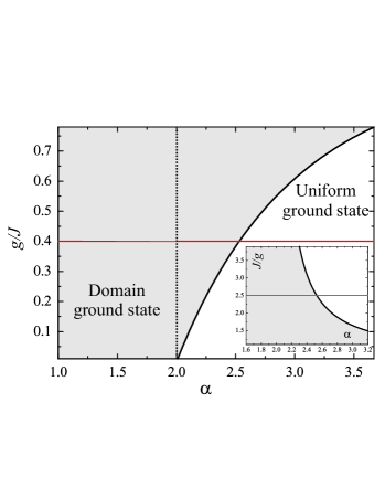
Figure 1: (Color online) Ground-state phase diagram in the $\left(\alpha\,,g/J\right)$ plane. For $1\leq\alpha\leq 2$ the ground state always consists of domains (grey region). For $\alpha>2$, the crossover to a uniform ground state (white region) occurs when $\alpha$ exceeds the threshold value $\alpha_{0}$ indicated by the solid line. MC calculations have been performed for values of $\alpha$ between 1.6 and 3.2 and $g/J=0.4$ (horizontal red line). Inset: zoom of the region where MC simulations have been performed in the $\left(\alpha\,,J/g\right)$ plane, $J/g=2.5$ (horizontal red line).

The zero-temperature phase diagram in the $\left(\alpha\,,g/J\right)$ plane is schematically reported in Fig. 1. The inset zooms into the region of the parameter space ($\left(\alpha\,,J/g\right)$ plane in this case) in which MC simulations have been performed: $J/g=2.5$ and $\alpha=1.6\dots 3.2$. The main thermodynamic observable we address is the two-point correlation function at temperature $T$ and fixed $\alpha$:

$$C_{\alpha}(r)=\langle\langle\sigma_{j+r}\sigma_{j}\rangle_{j}\rangle_{T}$$ (2)

and its Fourier transform $\mathcal{S}_{\alpha}(q)$ (commonly named structure factor):

$$\mathcal{S}_{\alpha}(q)=\sum_{r=-\infty}^{+\infty}\langle\langle\sigma_{j+r}\sigma_{j}\rangle_{j}\rangle_{T}e^{-iqr}\,.$$ (3)

As the system cannot be assumed to have translational invariance, an average over the lattice sites $j$ is needed ($\langle\dots\rangle_{j}$ in (2), (3) and henceforth); $\langle\dots\rangle_{T}$ denotes the thermal average. The physical quantities computed with the MC approach actually correspond to the double average $\langle\dots\rangle=\langle\langle\dots\rangle_{j}\rangle_{T}$.

The lowest-energy spin profiles are known to be square waves ${\rm Sq}(k_{0}j)$, with a modulation period $2h=2\pi/k_{0}$ Lieb . The total energy can be parameterized with $h$ by inserting the square profile into the Hamiltonian (1). The ground state equilibrium value of $h$ – let us call it $h_{gs}$, corresponding to $k_{gs}$ – is then determined by minimizing the resulting energy (20) with respect to $h$. $h_{gs}$ depends on $\alpha$ and $J/g$: some values are reported in Fig. 5. The two-point correlation function for a generic square-wave profile reads (see Appendix B for details):

$$\langle\sigma_{j+r}\sigma_{j}\rangle_{j} = \frac{1}{N}\sum_{j=1}^{N}{\rm Sq}(k_{0}(j+r)){\rm Sq}(k_{0}j)$$

$$= \frac{1}{2}\sum_{m=0}^{\infty}a^{2}_{m}\cos\left(k_{m}r\right)\doteq{\rm Tr}(k_{0}r)\,,$$

where $k_{0}=\pi/h$, $k_{m}=(2m+1)\cdot k_{0}$, $a_{m}=4\left[\pi(2m+1)\right]^{-1}$ and ${\rm Tr}(k_{0}r)$ is a symmetric triangular wave of period $2h$. According to (LABEL:GS_ss_derivation) evaluated in $h=h_{gs}$, the ground-state structure factor only takes non-zero values in the points located at $q=\pm(2m+1)\cdot k_{gs}$ for which $\mathcal{S}_{\alpha}\left((2m+1)\cdot k_{gs}\right)=N\cdot 4\left[\pi(2m+1)\right]^{-2}$. The structure factor of a uniform state takes a finite value at $q=0$ only: $\mathcal{S}_{\alpha}(0)=N$. This case can be regarded as the limit $h\rightarrow\infty$ so that $k_{0}=0$ and all the peaks of $\mathcal{S}_{\alpha}(k_{m})$ collapse into the peak at $q=0$.

II.2 Finite temperature

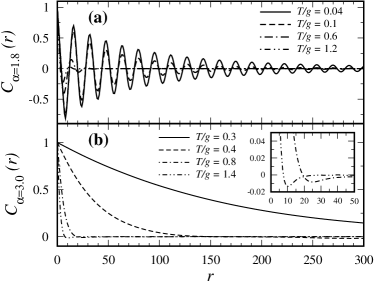
Figure 2: (a) Correlation function for $\alpha=1.8$ (domain ground state) at different temperatures for $L=1000$ and $J=2.5$. (b) Correlation function for $\alpha=3.0$ (uniform ground state) at different temperatures for $L=1000$ and $J=2.5$. Inset: Reminiscence of the competing dipolar interaction (see text).

Fig. 2 shows the two-point correlation functions (2) computed by MC simulations for $\alpha=1.8$ (domain ground state) and $\alpha=3.0$ (uniform ground state) at different temperatures (see Appendix A for details about the computational methods). In spite of the fact that the single-spin average $\langle\langle\sigma_{j}\rangle_{j}\rangle_{T}$ is zero at any finite temperature, the correlation function reproduces the essential aspects of the ground state spin configurations. For $\alpha=1.8$ (Fig. 2a), $C_{\alpha}(r)$ displays an oscillatory decay as a function of $r$, indicating that the loss of on-site magnetization proceeds in such a way that the ground-state segment-order is maintained. In the regime in which the ground state is uniform ($\alpha=3$), instead, the correlation function decays smoothly and, in general, monotonically (Fig. 2b). A closer look at the highest reported temperatures ($T/g=0.8\,,1.4$) reveals a small interval at short distances in which $C_{\alpha}(r)$ becomes negative (inset in Fig. 2b). This might be taken as an indication that, even starting from a uniform ground state, when the temperature is increased the system can spontaneously produce a phase with reduced symmetry in which the short-range order occurs with a well-defined modulation. We will come back to this point at the end of Section III.

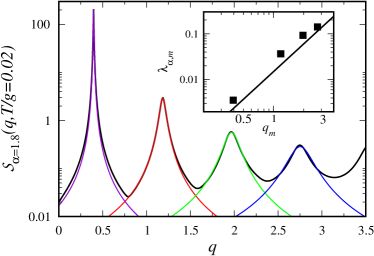
Figure 3: (Color online) Structure factor obtained by MC simulations at $T/g=0.02$ for $\alpha=1.8$ with Lorentzian fitting for the peaks located at $q=q_{m}=(2m+1)\cdot q_{\alpha,max}$ (and $J=2.5$). Inset: The HWHM $\lambda_{\alpha,m}$ obtained by Lorentzian fitting of the MC data (full squares) and given by formula (9) (line) is plotted versus $q_{m}$ in a log-log scale, which clearly reveals the power-law behavior.

In Fig. 3, the structure factor corresponding to $\alpha=1.8$ and $T=0.02$ is plotted. The set of discrete peaks of the ground state have broadened to Lorentzians centered at $q=(2m+1)\cdot q_{\alpha,max}$. Here, $q_{\alpha,max}$ means the position of the highest-peak of the simulated $\mathcal{S}_{\alpha}(q)$ at finite $T$ and does not, in general, coincide with $k_{gs}$ (the temperature dependence of $q_{\alpha,max}$ will be discussed below). The occurrence of multiple peaks in the finite-temperature structure factor not only indicates that the periodic structure of the ground state propagates at finite temperatures but also shows that some memory of the detailed square-wave spin profile is retained. As $T$ is increased, peaks with $m>0$ rapidly lose weight and, for $T\gtrsim 0.1$, basically only one peak is detectable. This implies a change of the correlation profile from triangular-wave-like (all harmonics) at low temperatures to cosine-like (single harmonic) at higher temperatures: the same cross-over is predicted to occur for the equilibrium mean-field spin profile within a 2d stripe-domain pattern and observed experimentally in the striped phase of ultra-thin Fe films grown epitaxially on Cu(001) Ale . Note that the height of the peaks of $\mathcal{S}_{\alpha}(q)$ in the ground state scales like $(2m+1)^{-2}$, while the ratio between the peaks at $m=1$ and $m=0$ in Fig. 3 is about one order of magnitude smaller at finite temperatures. In the next Section, we will give a simple explanation for this observation. The Lorentzian shape of the peaks and the $m$-dependence of their width (inset) – which are related to the exponential spatial dumping of the correlation shown in Fig. 2a – will also be discussed in Section III.

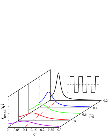
Figure 4: (Color online) Evolution of $\mathcal{S}_{\alpha}(q)$ as a function of temperature: The red dotted line represents the peak position $q_{\alpha,max}$ at different temperatures (parameters: $J/g=2.5$ and $\alpha=2.4$, giving $h_{gs}=51$). Inset: Schematic view of a square-wave spin profile.

A typical temperature dependence of the structure factor is shown in Fig. 4, using a linear scale where only the most prominent peak $m=0$ is evident. Two facts are visible: 1.) the location of the maximum $q_{\alpha,max}$ varies with temperature and 2.) the peak broadens considerably when the temperature is increased. We will discuss these two features more thoroughly.

II.2.1 Temperature and $\alpha$-dependence of $q_{\alpha,max}$

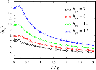
Figure 5: (Color online) Plot of $\langle h_{\alpha}\rangle$ versus $T/g$ in the domain-ground-state region. The computation parameters are $L=1000$, $J/g=2.5$, and $\alpha$ = 1.6 (circles), 1.8 (squares), 2 (diamonds), 2.2 (triangles). The statistical errors are smaller than the data symbols.

$\langle h_{\alpha}\rangle\doteq\pi/q_{\alpha,max}$ is plotted as a function of the temperature in Fig. 5 for the set of values $\alpha=1.6,1.8,2,2.2$, all in the regime $\alpha<\alpha_{0}$ for the chosen $J/g$. The ground-state value $h_{gs}$, found by minimizing the total energy (20) with respect to $h$, is also indicated. When $\alpha$ is increased – approaching the transition line to the uniform state – both ground-state and finite-temperature values also increase. A strongly decaying long-range interaction favors longer periods. To be more quantitative, two temperature regions have to be considered:

• For $T/J\gtrsim$0.3, the period of modulation decreases with temperature, in a similar way to what is found for the stripe width in the Mean-Field Approximation (MFA) of a similar but 2d model and in line with experimental results Ale .

• The temperature range $T/J\lesssim$0.3 is more difficult to explain. The modulation period saturates at the ground-state value for $\alpha=1.6,1.8$ and remains below the ground-state value for $\alpha=2.0,2.2$. We interpret the convergence of $\langle h_{\alpha}\rangle\rightarrow h_{gs}$ with $T\rightarrow 0$ as a positive indication that our MC calculations capture the essential equilibrium properties of the model, although we note that for larger periods, in this temperature range, the MC acceptance rate approaches zero (“blocked condition”). A further investigation should be required to decide whether this is due to a technical limitation or rather to the set-in of intrinsic slow dynamics, by analogy with similar systems Schmalian_Wolynes ; Cannas_slow_dyn_1 ; Cannas_slow_dyn_2 ; Cannas_slow_dyn_3 ; Cannas_slow_dyn_4 .
  

In Appendix D we will introduce an energy functional for finite $T$ which depends parametrically on the period of modulation $2h$. Within some approximations, there we show that the minimum of such a functional is found for smaller and smaller $h$ as the temperature is increased, thus reproducing qualitatively the dependence of $q_{\alpha,max}$ on $T$.

II.2.2 Temperature and $\alpha$-dependence of the correlation length $\xi_{\alpha}(T)\doteq\lambda_{\alpha,max}^{-1}$, $\lambda_{\alpha,max}$ being the Half Width at Half Maximum (HWHM) of the Lorentzian centered at $q_{\alpha,max}$

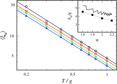
Figure 6: (Color online) Plot of $\xi_{\alpha}$ versus $T/g$ in the domain-ground-state region. The computation parameters are $L=$1000, $J/g=2.5$, and $\alpha$ = 1.6 (circles), 1.8 (squares), 2 (diamonds), 2.2 (triangles). The continuous lines represent the fit function $y=A_{\alpha}/x^{B_{\alpha}}$ (see text). The statistical errors are smaller than the data symbols. Inset: The values of $A_{\alpha}/g$ obtained by fitting the results of the MC simulations (main frame) are reported as a function of $\alpha$ (full squares connected by dotted line). The theoretical value of the prefactor of $1/T$ in formula (11), $(4/\pi^{2})h^{4}\left(\partial^{2}\mathcal{E}_{gs}/\partial h^{2}\right)$, is indicated by the solid “zig-zag” line (see text).

In Fig. 6, $\xi_{\alpha}$ is plotted versus $T/g$ for $\alpha=1.6,1.8,2,2.2$ (all falling in the region $\alpha\leq\alpha_{0}$ for $J/g=2.5$) in a log-log scale. Dots correspond to MC data while the solid lines represent fits with the function $A_{\alpha}/T^{B_{\alpha}}$, with fitting parameters $A_{\alpha}$ and $B_{\alpha}$. The best fit yields the same exponent $B_{\alpha}=1.10(5)$ for each $\alpha$, while $A_{\alpha}$ has a more complicated dependence on $\alpha$, see squares in the inset of Fig. 6 (the zig-zag line will be discussed in the next Section). We conclude that the dependence of the correlation length on $T$ is better described by $A_{\alpha}/T^{B_{\alpha}}$ than the Ising exponential relation $e^{\Delta/T}$, which holds for $g=0$. A deeper understanding of this difference will be provided in Section III. For a comparison with the uniform regime (i.e., $\alpha=2.6,2.8,3,3.2$), let us consider the correlation function for $\alpha=3.0$ displayed in Fig. 2b. Note that the plot is limited to low enough temperatures in order to avoid the anomalous range of spatial decay where the correlation function becomes negative (see inset of Fig. 2b).

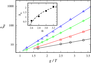
Figure 7: (Color online) Log-linear plot of $\xi_{\alpha}$ versus $g/T$ in the uniform-ground-state region. The computation parameters are $L=1000$, $J/g=2.5$, and $\alpha$ = 2.6 (circles), 2.8 (squares),  3.0 (diamonds), 3.2 (triangles). The continuous lines are best fit functions. The statistical errors are smaller than the data symbols. Inset: The dependence of the barrier $\Delta_{w}=2J-2g\zeta(\alpha-1)$ derived in Sect. III on $\alpha$ (dashed line) is compared with that of $\Delta_{\alpha}$ obtained by fitting $\xi_{\alpha}$ computed in MC simulations (full squares).

Besides, in the temperature range $T=0.3\dots 0.8$, the $g=0$ behavior is recovered. In fact, looking at the correlation length $\xi_{\alpha}$ for $\alpha=2.6,2.8,3,3.2$, we find that it is better fitted by $\xi_{\alpha}\sim\exp\left(\Delta_{\alpha}/T\right)$, see the log-linear plot of $\xi_{\alpha}$ versus $g/T$ in Fig. 7. Remarkably, the energy barrier $\Delta_{\alpha}$ does depend on $\alpha$, see squares in the inset of Fig. 7 (the dashed line will be discussed at the end of the next Section).

Regarding the possibility to observe long-range order at finite temperature, our MC results seem to exclude such a hypothesis. In fact, in a correct analysis of the structure factor, beyond the usual intensive term connected with the correlations (Lorenzian-like functions), one should also take into account an extensive factor associated with the occurrence of long-range order chailub . This last component has always been considered in the fitting procedure but it has never given a significant contribution to the simulated structure factors (3). The occurrence of long-range order at $T=0$ only is also supported by the low-temperature divergence of $\xi_{\alpha}$ for both $\alpha\leq\alpha_{0}$ (Fig. 6) and $\alpha>\alpha_{0}$ (Fig. 7). The whole scenario confirms some recent theoretical works. In fact, in Ref. kerimov, the absence of long-range order at any temperature for $g>0$, $J=0$ and $\alpha>1$ is rigorously proved. Even if in that specific case a short-range ferromagnetic term was not included, it seems reasonable to extend such a result to the case $J>0$ and conclude that long-range order should not occur with the model (1) for $\alpha>1$ Lieb . The occurrence of a phase transition has been suggested, instead, for $0<\alpha\leq 1$ so that it would be particularly interesting to investigate the finite-temperature properties of the model (1) in this regime. However, several other issues are related to the divergence of the energy per spin for pair-spin interaction decaying like $1/r^{\alpha}$ with $\alpha<d$, $d$ being the dimension of the space in which the spin system is embedded, such as energy non-additivity and ensemble inequivalence Ruffo_2 ; barre05 ; mukamel . For this reason our canonical MC method would not necessarily provide the unique and correct results in this context, but further analyses involving the comparison of different computational approaches would be, most probably, required.

III Discussion

In this Section, we provide an explanation for some of the MC results on the basis of a simple physical model for the excited states of the Hamiltonian (1). In particular, we will provide a physical picture for the temperature dependence of the correlation length in the two distinct regimes $\alpha\leq\alpha_{0}$ and $\alpha>\alpha_{0}$.

III.1 Case $\alpha\leq\alpha_{0}$

We construct excited states of the Hamiltonian (1) by modifying the square-wave profile to

$$\sigma_{j}={\rm Sq}\left(k_{0}(j+u_{j})\right)=\sum_{m=0}^{\infty}a_{m}\sin\left(k_{m}(j+u_{j})\right)$$ (5)

with $u_{j}$ being a displacement field. This perturbation corresponds to displacing the position of the wall between adjacent segments, which creates a generally non-periodic spin configuration. The quantity we need to compute is the increment of energy due to the displacement field:

$$\Delta\mathcal{E}_{h}\doteq\mathcal{E}_{h}[u]-\mathcal{E}_{h}[u=0]$$ (6)

with $\mathcal{E}_{h}$ being defined as $\langle\mathcal{H}\rangle_{j}$. $\Delta\mathcal{E}_{h}$ is computed perturbatively, i.e., in the limit of small $\tilde{u}_{q}$ ($u_{j}\doteq\left(1/N\right)\sum_{q}\tilde{u}_{q}e^{iqj}$), see Appendix C. For $q<<k_{0}$ and setting $k_{0}=k_{gs}$, with $k_{gs}$ being $\pi/h_{gs}$, one has

$$\Delta\mathcal{E}_{gs}=\frac{1}{N}\sum_{q}\left[\frac{1}{2}k_{gs}^{2}\frac{\partial^{2}\mathcal{E}_{gs}}{\partial k_{0}^{2}}q^{2}|\tilde{u}_{q}|^{2}\right]\,.$$ (7)

Eq. (7) describes the spectrum of the excited states (see also Refs. Kashuba_Pokrovsky, ; Abanov_Pokrovsky, for a model in 2d) and the coefficient of $q^{2}$ is a stiffness $k_{gs}^{2}\left(\partial^{2}\mathcal{E}_{gs}/\partial k_{0}^{2}\right)$ against fluctuations from the ground-state spin configuration (see Appendix C for $\partial^{2}\mathcal{E}_{gs}/\partial k_{0}^{2}$ definition). Note the gapless, quasi-continuum nature of the spectrum of fluctuations, in clear contrast to the gapped spectrum of fluctuations in a pure ($g=0$) Ising model.

Eq. (7) is the central result of this Section, as it allows computing the structure factor $\mathcal{S}_{\alpha}(q)$ and the correlation length $\xi_{\alpha}(T)$. The resulting structure factor (3) consists of a series of Lorentzian peaks centered at $q=\pm k_{m}$

$$\mathcal{S}_{\alpha}(q) = \frac{1}{2}\sum_{m=0}^{\infty}\Bigg{\{}a^{2}_{m}$$

$$\times \left.\left[\frac{\lambda_{\alpha,m}}{\left(q-k_{m}\right)^{2}+\lambda_{\alpha,m}^{2}}+\frac{\lambda_{\alpha,m}}{\left(q+k_{m}\right)^{2}+\lambda_{\alpha,m}^{2}}\right]\right\}\,,$$

with a HWHM given by

$$\lambda_{\alpha,m}=(2m+1)^{2}\frac{T}{2\frac{\partial^{2}\mathcal{E}_{gs}}{\partial k_{0}^{2}}}\,.$$ (9)

The reader is referred to Appendix C for the details. The same behavior is observed in the MC results plotted in Fig. 3. Our analysis finds the origin of the multiple peaks of $\mathcal{S}_{\alpha}(q)$ in the quasi-continuum spectrum of gapless excitations (see Eq. (7)) appearing in the frustrated model for $\alpha\leq\alpha_{0}$. A remarkable feature is the non-trivial scaling of the maxima with the higher-harmonic index $2m+1$

$$\mathcal{S}_{\alpha}(q=\pm k_{m})=\frac{1}{2}\frac{a_{m}^{2}}{\lambda_{\alpha,m}}=\frac{16}{\pi^{2}}\frac{\partial^{2}\mathcal{E}_{gs}}{\partial k_{0}^{2}}\frac{1}{T}\frac{1}{(2m+1)^{4}}\,,$$ (10)

which accounts for the strong reduction detected for the ratio between the peak heights for $m=1$ and $m=0$ in the MC results at finite temperatures. Note also the square-power dependence of the HWHM $\lambda_{\alpha,m}$ on $2m+1$ in formula (9). This theoretical prediction (solid line in the inset of Fig. 3 with log-log scale) is in excellent agreement with the behavior of the $\mathcal{S}_{\alpha}(q)$ simulated for $\alpha=1.8$ and $J/g=2.5$ at $T/g=0.02$ (squares in the inset of Fig. 3). From the assumption $k_{0}=k_{gs}$ (Eq. (7)) it follows that, within our analytic model, the highest peak of $\mathcal{S}_{\alpha}(q)$ is expected to occur at $q_{\alpha,max}=k_{gs}$ and the correlation length is defined as $\xi_{\alpha}=\lambda_{\alpha,0}^{-1}$ consistently. Even if we already know that in MC simulations $q_{\alpha,max}$ does not remain constant as $T$ is varied (see Fig. 5), this assumption produces a $1/T$-dependence of the correlation length

$$\xi_{\alpha}=\frac{1}{\lambda_{\alpha,0}}=2\frac{\partial^{2}\mathcal{E}_{gs}}{\partial k_{0}^{2}}\frac{1}{T}\,,$$ (11)

which is in good agreement ($B_{\alpha}=1.10(5)$) with the corresponding quantity computed again with the MC technique (see Fig. 6). Finally, the analytic model predicts that $A_{\alpha}=2\left(\partial^{2}\mathcal{E}_{gs}/\partial k_{0}^{2}\right)$. Computing this expression numerically produces the solid curve in the inset of Fig. 6. The step-like behavior of $2\left(\partial^{2}\mathcal{E}_{gs}/\partial k_{0}^{2}\right)$ reflects the fact that both the optimal domain width $h_{gs}$ and the second derivative of the energy – computed in $h=h_{gs}$ – are discontinuous functions of $\alpha$ Lieb in virtue of the discreteness of the lattice. Both the order of magnitude and the scaling with $\alpha$ agree with MC calculations (squares in the inset of Fig. 6): $A_{\alpha}$ decreases as $\alpha$ increases approaching the uniform-ground-state region. In summary, the agreement between numerical and analytical results indicates that the distortion of the ground-state spin profile due to the displacement of domain walls represents the main disordering mechanism when $\alpha\leq\alpha_{0}$.
To the aim of reproducing the temperature dependence of $q_{\alpha,max}$, the expansion for $q\ll k_{0}$ – performed in Appendix C to get from (LABEL:DFIF_perturb_energy_4_app_B) to (33) – is not expected to be accurate anymore. However, in Appendix D we show that letting $h$ be an adjustable parameter at finite $T$ with an appropriate (temperature-dependent) stiffness we are able to reproduce qualitatively the decrease of the modulation period with increasing temperature observed in MC simulations. This, indeed, happens because in the correlation function (41) higher harmonics are progressively more suppressed as the temperature increases. As a result, the competition between the ferromagnetic exchange and the antiferromagnetic long-range interaction turns out to be biassed with respect to the zero-temperature case and the period of modulation decreases subsequently. This close relationship between the suppression of higher-harmonic components and the decrease of the characteristic period of modulation has been already highlighted experimentally and by mean-field calculations in an equivalent 2d system, suggesting that it might be a general property of such models.

The pure Ising Hamiltonian is invariant with respect to any operation that changes the variable $\sigma_{j}$ to $-\sigma_{j}$: it has the discrete symmetry group $\mathbb{Z}_{\,2}$. In the next Subsection, we will discuss this case in connection with $\alpha>\alpha_{0}$. The $1/T$-dependence of the correlation length, obtained by introducing a long-range interaction ($g\neq 0$), suggests that, in the regime of $\alpha\leq\alpha_{0}$, the frustrated system crosses over to the completely different universality class of one-dimensional chains hosting a planar spin field with SO(2) continuous symmetry Wegner ; Fisher .

III.2 Case $\alpha>\alpha_{0}$

In this regime, the ground state is uniform and the Ising universality class is restored at low enough temperatures, as shown by the correlation length diverging exponentially as $e^{\Delta/T}$, see Fig. 7. Specific to this case is that $\Delta=\Delta_{\alpha}$, see Inset Fig. 7. We try to explain this result by considering that, in the pure Ising model ($g=0$), the barrier $\Delta$ equals the energy cost to reverse half of the spins starting from a uniform configuration. Were the general arguments which associate such an energy with the low-temperature expansion of $\xi$ Shriffer applicable in the presence of long-range interaction, the energy of a single wall would be expected to equal $\Delta_{\alpha}$. When half of the spins in the chain are reversed, the exchange energy increases by $2J$. To compute the variation due to the long-range interaction, note that this interaction energy is just given by twice the interaction energy between the two parts of the chains lying on opposite sides with respect to the domain wall (as the self-energy in each domain remains the same before and after the flip of half of the spins). This interaction energy is given by

$$\Delta_{g}=-2g\sum_{j\geq 0}\sum_{i\geq 1}\frac{1}{|j+i|^{\alpha}}=-2g\sum_{r\geq 1}\frac{r}{r^{\alpha}}=-2g\zeta(\alpha-1)\,,$$ (12)

where $\zeta(x)$ is the Riemann zeta function, while $i$ and $j$ are the site indices of spins lying on opposite sides of the domain wall. The energy to create a wall becomes explicitly dependent on $\alpha$ and amounts to $\Delta_{w}=2J-2g\zeta(\alpha-1)$. In the inset of Fig. 7, one can appreciate how this estimate actually reproduces both the order of magnitude and the dependence on $\alpha$ of the energy barrier of the exponentially diverging $\xi_{\alpha}$ obtained from MC simulations. To be rigorous, one should point out that this approach is not completely justified in this context since, when a long-range interaction is present, the creation of a new domain wall is not statistically independent of the number and the location of the pre-existing domain walls in the chain; such a hypothesis is indeed a basic assumption to put the correlation length in relationship with the cost to create a single wall in the system Shriffer . Letting $\alpha$ go to infinity effectively reduces the spin-spin interaction to nearest neighbors only so that our system becomes equivalent to the usual Ising model, provided that the exchange interaction is replaced by $J-g$.

At $T=0$, the condition $\Delta_{w}=0$ defines $\alpha_{0}$. In fact, as soon as $\Delta_{w}\leq 0$ the uniform configuration has no more the lowest energy and the system prefers to split into domains. For a given ratio $J/g$, $\alpha_{0}$ fulfills the condition $\zeta(\alpha_{0}-1)=J/g$. Using the integral definition of the Riemann zeta function, the previous condition can be rewritten as

$$\frac{J}{g} = \zeta(\alpha_{0}-1)=\frac{1}{\Gamma(\alpha_{0}-1)}\int^{\infty}_{0}dx\frac{x^{\alpha_{0}-2}}{e^{x}-1}$$

$$= \frac{1}{\alpha_{0}-1}\frac{1}{\Gamma(\alpha_{0}-1)}\int^{\infty}_{0}dx\frac{x^{\alpha_{0}-1}e^{x}}{(e^{x}-1)^{2}}$$

$$= \frac{1}{\Gamma(\alpha_{0})}\int^{\infty}_{0}dx\frac{x^{\alpha_{0}-1}e^{-x}}{(1-e^{-2x})^{2}}\,;$$

this implicit equation for $\alpha_{0}$ turns out to be exact Lieb (the solution being the solid line in Fig. 1).

For completeness, we recall that at relatively high temperatures a well-defined period of modulation seems to emerge in the correlation function also for $\alpha>\alpha_{0}$ (see inset of Fig. 2b). A naïve, but essentially correct, interpretation of the temperature dependence of $q_{\alpha,max}$ in the regime $\alpha\leq\alpha_{0}$ suggests that thermal fluctuations effectively reduce the ratio $J/g$ (the antiferromagnetic long-range interaction is fovored in the competition with the ferromagnetic exchange interaction, which finally leads to decrease the modulation period with respect to the $T=0$ case). In this sense, one may think that even when the uniform pattern has the minimum energy at $T=0$ (e.g. for $J/g=2.5$ and $\alpha=3$ as in Fig. 2b), thermal fluctuations induce an effective decrease of the ratio $J/g=2.5$ so that a modulated phase eventually has lower free energy at high enough temperatures. However, this effect can only be evident if such a crossover occurs when there is still enough correlation between spins to develop – at least – half-period of modulation, i.e. roughly for $\xi_{\alpha}>1/q_{\alpha,max}$. In fact, if the period of the underlying modulated phase is much larger than the correlation length $\xi_{\alpha}$, two-point correlations just display a monotonic decay as a function of the lattice separation. A detailed investigation of this phenomenon would be, indeed, intriguing but it is beyond the purpose of the present work.

IV Conclusions

The Mean-Field Approximation reported e.g. in Ref. Ale, provides some straightforward results concerning ferromagnetic Ising system frustrated by a long-range interaction. However, the MFA fails in one important instance: it predicts that the modulated order in the ground state propagates at finite temperatures up to a second-order transition temperature $T_{c}$, while the Landau-Peierls instability forbids a finite on-site $\langle\sigma_{j}\rangle_{T}$ at any finite temperature Landau_Lifshitz ; Peierls . On the other side, MC simulations are much more accurate than the MFA, but very difficult to perform under experimentally realistic conditions. For instance, the large modulation lengths often observed in experiments are practically inaccessible to MC simulations. We concentrated on a model – Eq. (1) – that is highly simplified but captures some essential characteristics of some physically relevant two-dimensional frustrated systems. Within this model, we have been able to enlarge the modulation length with respect to full two-dimensional MC simulations Cannas_Pighin ; Rastelli . With this model, we have obtained a set of results that might help to shed light onto some experimental outcomes. In particular: The modulation length appearing in the ground state is found to remain a characteristic length at finite temperatures, where it appears as the length modulating the oscillatory part of the correlation function. Strikingly, it decays with temperature in a way that is similar to the temperature dependence of the stripe-domain width observed in MFA and experimentally on Fe/Cu(001) films Ale ; Oliver1 . In addition, the spatial profile of the correlation function contains the same kind of higher harmonics appearing in the MFA spin profile, with only one fundamental harmonic remaining at sufficiently high temperatures, as specified within the MFA and found experimentally Ale . In contrast to the MFA, which predicts a second-order phase transition also in 1d, we do not find any trace of a phase transition – and this is a major deviation from full two-dimensional MC simulations Cannas_Pighin ; Rastelli or experimental findings. When the spatial decay of the long-range interaction is too short-ranged, the ground state and the finite-temperature state lose the modulated character and become uniform. Correspondingly, the system crosses over from the universality class proper of 1d systems with continuous symmetry Wegner ; Fisher to the standard 1d Ising-like universality class Ising ; Huang .
For future work, a more accurate treatment of the displacement field $u_{j}$ beyond the $q\ll k_{0}$ approximation (see Appendix C) is certainly to be considered.

Appendix A Monte Carlo Method

In this Appendix, we discuss the technical details of the MC method we used to study the finite-temperature properties of the Hamiltonian (1). A first important issue for the system under investigation is the treatment of finite-size effects. In the presence of long-range interactions, they need to be handled with particular care both numerically and analytically Ruffo . Some techniques to tackle the problem numerically are given, for instance, in Ref. libbinder, . We perform our simulations on a system containing $L$ spins and treat the long-range effects by replicating many identical copies of the “simulation box” Cannas_Lapilli . More explicitly, the interaction between two spins separated by $r$ lattice sites reads

$$G_{\alpha}(r)=\frac{1}{r^{\alpha}}+\sum_{n}\frac{1}{|r+nL|^{\alpha}}\,,$$ (14)

where the index $n$ accounts for the number $N/L$ of replicated boxes. Since we have in mind the thermodynamic limit $N\rightarrow\infty$, for numerical evaluation of $G_{\alpha}(r)$ we let $n$ go to $\pm\infty$ in order to account for the copies of the system lying on both the left- and right-hand sides of the simulated segment, containing just $L$ spins. The effective coupling (14) can be rewritten, in a way that is more suitable for computational purposes:

$$G_{\alpha}(r) = \frac{1}{r^{\alpha}}+\sum_{n=\pm 1\dots\pm\infty}\frac{1}{|r+nL|^{\alpha}}$$

$$= \frac{1}{r^{\alpha}}+\sum_{n=1}^{\infty}\left[\frac{1}{|r+nL|^{\alpha}}+\frac{1}{|r-nL|^{\alpha}}\right]$$

$$= \frac{1}{r^{\alpha}}+\frac{1}{L^{\alpha}}\left\{\sum_{n=1}^{M}\left[\frac{1}{|n+\frac{r}{L}|^{\alpha}}+\frac{1}{|n-\frac{r}{L}|^{\alpha}}\right]\right.$$

$$+ \left.\sum_{n=M+1}^{\infty}\left[\frac{1}{|n+\frac{r}{L}|^{\alpha}}+\frac{1}{|n-\frac{r}{L}|^{\alpha}}\right]\right\}$$

$$\simeq \frac{1}{r^{\alpha}}+\frac{1}{L^{\alpha}}\left\{\sum_{n=1}^{M}\left[\frac{1}{|n+\frac{r}{L}|^{\alpha}}+\frac{1}{|n-\frac{r}{L}|^{\alpha}}\right]\right.$$

$$+ \left.2\sum_{n=M+1}^{\infty}\frac{1}{n^{\alpha}}\right\}=\frac{1}{r^{\alpha}}+\frac{2\zeta(\alpha)}{L^{\alpha}}$$

$$+ \frac{1}{L^{\alpha}}\sum_{n=1}^{M}\left[\frac{1}{|n+\frac{r}{L}|^{\alpha}}+\frac{1}{|n-\frac{r}{L}|^{\alpha}}-\frac{2}{n^{\alpha}}\right]\,;$$

in the third passage we have neglected $r/L$ with respect to $M$; the error of the whole approximation can be estimated following Ref. Cannas_Lapilli, . This approximation reduces the main computational task to evaluating the finite sum over $n$, which is – however – rapidly convergent. Finally, the working Hamiltonian, restricted to our simulation box, is given by

$$\mathcal{H}=-J\sum_{i=1}^{L}\sigma_{i}\sigma_{i+1}+\frac{g}{2}\sum_{i=1}^{L}\sum_{j=1}^{L}\sigma_{i}\sigma_{j}G_{\alpha}(i-j)\,,$$ (16)

which descends directly from (1) with the replica assumption $\sigma_{i\pm nL}=\sigma_{i}$ ($n=\pm 1\dots\pm\infty$), periodic boundary conditions on the simulation box $\sigma_{L+1}=\sigma_{1}$ and setting $r=|i-j|$. Note that the indices $i$ and $j$ now vary in the range $[1,L]$ and are allowed to be equal, $G_{\alpha}(0)$ being representative of the interaction between different spins in the original Hamiltonian (1); in this particular case ($r=0$), there is no interaction inside the simulation box but the $i$-th spin still interacts with its own copies lying in the different replicas, $\sigma_{i\pm nL}$, so that

$$G_{\alpha}(0)=\sum_{n=\pm 1\dots\pm\infty}\frac{1}{|nL|^{\alpha}}=\frac{2\zeta(\alpha)}{L^{\alpha}}\,.$$ (17)

The MC simulations have been performed using the Simulated Annealing (SA) opsa paradigm. The SA is extensively applied in statistical physics with the intent to study systems where both the ground-state energy and the equilibrium at low temperatures are inaccessible through the basic Metropolis criterion libbinder . Certainly, spin glasses spinglass , frustrated magnetic spin structures Diep and models with long-range interactions Ruffo are some typical examples of systems where the SA and related methods Santoro are largely exploited.

We also have to remind that in literature some cluster methods were employed in order to reach a correct thermodynamic equilibrium for a simple model where ferromagnetic long-range interactions are only present cluster . However, the strong frustration due to the competition between the antiferromagnetic long-range interactions and the nearest-neighbor ferromagnetic exchange interaction renders the generalization of such cluster MC technique to the present case non-trivial. For these reason, we have followed in this work the main idea of Kirkpatrick et al. opsa . A random initial configuration (which should be considered as a paramagnetic state) is picked up. Subsequently, the thermodynamic equilibrium at a high enough temperature $T_{0}$ is established. We remember that the MC steps per spin considered here only comprise Metropolis moves at the analyzed temperature. $T_{0}$ is usually chosen in order to have a high MC acceptance ratio per spin. Then the temperature is decreased gradually $T\rightarrow T-\Delta T$ ($\Delta T>0$), and a fixed number of MC steps per spin $\tau$ is run, starting with the last configuration sampled at the previous higher temperature. So, the main assumption is to force a constant and sufficiently slow cooling rate, defined as $r=\Delta T/\tau$. We have taken $\Delta T=0.1\dots 0.001$ and $\tau=1\dots 5\times 10^{5}$ depending on the studied value of $\alpha$. The procedure is completed when the ground state is approached.

We have considered simulation boxes of size $L$=100, 200, 500, 1000, and 2000. After discarding the first 1$\times$10⁵ MC steps, we have collected between 5$\times$10⁵ and 1$\times$10⁶ measurements of the thermodynamic observables, repeating the simulation for each temperature at least three times. The estimation of the statistical errors has been achieved by applying the usual blocking technique libbinder .

Appendix B Correlations in the ground state

In this Appendix, we compute the two-point correlations for a generic square-wave spin profile, representative of the regime in which the ground state consists of domains: $\alpha\leq\alpha_{0}$. The lowest-energy configurations, at $T=0$, are known to be given Lieb by square-wave spin profiles

$$\sigma_{j}={\rm Sq}(k_{0}j)=\sum_{m=0}^{\infty}a_{m}\sin\left(k_{m}j\right)$$ (18)

with $k_{0}=\pi/h$, $k_{m}=\pi(2m+1)/h$ and $a_{m}=4/\left[\pi\left(2m+1\right)\right]$. With the orthogonality relation $\sum_{j=1}^{N}e^{-i(k-k^{\prime})j}=N\delta_{k,k^{\prime}}$, the two-point correlations averaged over the site variables $j$ can be computed:

$$\langle\sigma_{j+r}\sigma_{j}\rangle_{j}=\frac{1}{N}\sum_{j=1}^{N}{\rm Sq}(k_{0}(j+r)){\rm Sq}(k_{0}j)$$

$$=\frac{1}{N}\sum_{j=1}^{N}\sum_{m,m^{\prime}=0}^{\infty}a_{m^{\prime}}a_{m}\sin\left(k_{m}(j+r)\right)\sin\left(k_{m^{\prime}}j\right)$$

$$=\frac{1}{2}\sum_{m=0}^{\infty}a^{2}_{m}\cos\left(k_{m}r\right)\,.$$

(19)

The Fourier coefficients of the series obtained in the final passage of equation (19) happen to be the same as for the symmetric triangular wave of period $2h$ so that in the text we use the compact notation $\langle\sigma_{j+r}\sigma_{j}\rangle_{j}={\rm Tr}(k_{0}r)$.
Eq. (19) allows writing the energy per spin for a general square-wave profile

$$\mathcal{E}_{h} = -J\,{\rm Tr}(k_{0})+\frac{g}{2}\sum_{m=0}^{\infty}a^{2}_{m}\sum_{r\geq 1}\frac{\cos\left(k_{m}r\right)}{r^{\alpha}}$$

$$= \sum_{m=0}^{\infty}a^{2}_{m}f_{\alpha}(k_{m})\,,$$

(20)

which depends parametrically on the half-period of modulation $h$. The ground-state energy for a given ratio $J/g$ and $\alpha$ can be obtained by minimizing equation (20) with respect to $h$ numerically, which consequently defines the equilibrium domain width $h_{gs}$ at $T=0$. The exchange term in (20) straightforwardly gives $-J\,{\rm Tr}(k_{0})=-J\left(1-2/h\right)$, also deducible by counting the number of walls present in the domain configuration with modulation period $2h$. The function $f_{\alpha}(k_{m})=-\left(J/2\right)\cos\left(k_{m}\right)+g/2\sum_{r\geq 1}\left(\cos\left(k_{m}r\right)/r^{\alpha}\right)$ introduced above will be used to write the perturbed energy in a more compact form.

Appendix C Perturbative treatment of correlations at finite temperatures

In this Appendix, we develop a perturbative elastic model which allows us to compute the two-point correlations in the regime $\alpha\leq\alpha_{0}$ at finite temperatures. Let us consider a displacement field, $u_{j}$, of the whole square-wave profile (18):

$$\sigma_{j}={\rm Sq}\left(k_{0}(j+u_{j})\right)=\sum_{m=0}^{\infty}a_{m}\sin\left(k_{m}(j+u_{j})\right)\,.$$ (21)

To compute how the energy (19) is modified by the presence of this elementary perturbation, we introduce the constants

$$\begin{cases}&a=k_{m}(j+r)\\ &b=k_{m^{\prime}}j\end{cases}\quad\quad\quad\begin{cases}&\gamma=k_{m}u_{j+r}\\ &\beta=k_{m^{\prime}}u_{j}\end{cases}$$ (22)

where the two Greek letters will henceforth be assumed infinitesimal. Eq. (19) then involves terms like

$$\sin(a+\gamma)\sin(b+\beta)=\sin a\sin b\cos\gamma\cos\beta$$

$$+ \sin a\cos b\cos\gamma\sin\beta+\cos a\sin b\sin\gamma\cos\beta$$

$$+ \cos a\cos b\sin\gamma\sin\beta\,.$$

We will further assume that the average over the lattice indices $j$, $\langle\dots\rangle_{j}$, can be performed independently for the rigid pattern variables (Latin letters) and for the fluctuating displacement field $u_{j}$ :

$$\begin{split}\langle\sin a\sin b\cos\gamma\cos\beta\rangle_{j}=\langle\sin a\sin b\rangle_{j}\langle\cos\gamma\cos\beta\rangle_{j}\,.\end{split}$$ (24)

The average $\langle\dots\rangle_{j}$ for elementary trigonometric functions with arguments $a$ and $b$ gives:

$$\begin{cases}&\langle\sin a\sin b\rangle_{j}=\langle\cos a\cos b\rangle_{j}=\frac{1}{2}\delta_{m,m^{\prime}}\cos\left(k_{m}r\right)\\ &\langle\sin a\cos b\rangle_{j}=-\langle\cos a\sin b\rangle_{j}=\frac{1}{2}\delta_{m,m^{\prime}}\sin\left(k_{m}r\right)\,,\end{cases}$$ (25)

which can be exploited to average (LABEL:sin_sin_prod_u_app_B) with respect to $j$:

$$\langle\sin(a+\gamma)\sin(b+\beta)\rangle_{j}$$

$$=\frac{1}{2}\delta_{m,m^{\prime}}\cos\left(k_{m}r\right)\langle\cos\gamma\cos\beta+\sin\gamma\sin\beta\rangle_{j}$$

$$+\frac{1}{2}\delta_{m,m^{\prime}}\sin\left(k_{m}r\right)\langle\cos\gamma\sin\beta-\sin\gamma\cos\beta\rangle_{j}$$

$$=\frac{1}{2}\delta_{m,m^{\prime}}\left\{\cos\left(k_{m}r\right)\langle\mathcal{R}e\left[e^{i(\beta-\gamma)}\right]\rangle_{j}\right.$$

$$\left.+\sin\left(k_{m}r\right)\langle\mathcal{I}m\left[e^{i(\beta-\gamma)}\right]\rangle_{j}\right\}\,;$$

then, recalling that $\beta-\gamma=k_{m}\left(u_{j}-u_{j+r}\right)$, we get:

$$\langle\sigma_{j+r}\sigma_{j}\rangle_{j} =\frac{1}{2}\sum_{m=0}^{\infty}\left\{a^{2}_{m}\left(\cos\left(k_{m}r\right)\langle\mathcal{R}e\left[e^{ik_{m}\left(u_{j}-u_{j+r}\right)}\right]\rangle_{j}\right.\right.$$

$$\qquad\qquad+\left.\left.\sin\left(k_{m}r\right)\langle\mathcal{I}m\left[e^{ik_{m}\left(u_{j}-u_{j+r}\right)}\right]\rangle_{j}\right)\right\}\,.$$

The introduction of the displacement field brings an increment to the energy of a general square-wave profile (20) equal to

$$\Delta\mathcal{E}_{h} = -J\frac{1}{2}\sum_{m=0}^{\infty}\langle a^{2}_{m}\left[\sin\left(k_{m}\right)\sin\left[k_{m}(u_{j}-u_{j+1})\right]\right.\left.+\cos\left(k_{m}\right)\left(\cos\left[k_{m}(u_{j}-u_{j+1})\right]-1\right)\right]\rangle_{j}$$

$$+ \frac{g}{2}\sum_{m=0}^{\infty}\langle a^{2}_{m}\sum_{r\geq 1}\left[\frac{\sin\left(k_{m}r\right)}{r^{\alpha}}\sin\left[k_{m}(u_{j}-u_{j+r})\right]\right.\left.+\frac{\cos\left(k_{m}r\right)}{r^{\alpha}}\left(\cos\left[k_{m}(u_{j}-u_{j+r})\right]-1\right)\right]\rangle_{j}$$

$$\simeq -J\frac{1}{2}\sum_{m=0}^{\infty}\langle a^{2}_{m}\left[-\sin\left(k_{m}\right)k_{m}(u_{j+1}-u_{j})\right.\left.-\frac{1}{2}\cos\left(k_{m}\right)k_{m}^{2}\left(u_{j+1}-u_{j}\right)^{2}\right]\rangle_{j}$$

$$+ \frac{g}{2}\sum_{m=0}^{\infty}\langle a^{2}_{m}\sum_{r\geq 1}\left[-\frac{\sin\left(k_{m}r\right)}{r^{\alpha}}k_{m}(u_{j+r}-u_{j})\right.\left.-\frac{1}{2}\frac{\cos\left(k_{m}r\right)}{r^{\alpha}}k_{m}^{2}\left(u_{j+r}-u_{j}\right)^{2}\right]\rangle_{j}\,,$$

where we have expanded the energy for small displacement differences $u_{j+r}-u_{j}$.

To proceed in our calculation it is convenient to express the displacement field in terms of its Fourier transform $\tilde{u}_{q}$:

$$u_{j}=\frac{1}{N}\sum_{q}\tilde{u}_{q}e^{iqj}\quad\quad{\rm with}\quad\quad\tilde{u}_{q}=\sum_{j}u_{j}e^{-iqj}\,,$$ (29)

the sum is performed over the Fourier wave numbers $q_{m}=\pm\left(2\pi m\right)/N$ with $m\in[-N/2,N/2]$, but we drop the index $m$ for simplicity. From Eq. (29) it follows that the averaged square difference is

$$\langle\left(u_{j+r}-u_{j}\right)^{2}\rangle_{j}=\frac{2}{N}\sum_{q}|\tilde{u}_{q}|^{2}\left[1-\cos(qr)\right]\,,$$ (30)

while $\langle u_{j+r}-u_{j}\rangle_{j}=0$. The previous results and the elementary trigonometric relation $\cos(x)\cos(y)=\left(1/2\right)\left[\cos(x-y)+\cos(x+y)\right]$ allow writing (LABEL:DFIF_perturb_energy_app_B) as

$$\Delta\mathcal{E}_{h} = \frac{1}{N}\sum_{q}\frac{J}{2}\sum_{m=0}^{\infty}\left\{a^{2}_{m}k_{m}^{2}\left[\cos(k_{m})-\frac{1}{2}\cos(k_{m}-q)-\frac{1}{2}\cos(k_{m}+q)\right]|\tilde{u}_{q}|^{2}\right\}$$

$$- \frac{1}{N}\sum_{q}\frac{g}{2}\sum_{m=0}^{\infty}\left\{a^{2}_{m}k_{m}^{2}\frac{1}{2}\sum_{r\geq 1}\frac{1}{r^{\alpha}}\left[\cos(k_{m}r)\right.\left.-\frac{1}{2}\cos\left[(k_{m}-q)r\right]-\frac{1}{2}\cos\left[(k_{m}+q)r\right]\right]|\tilde{u}_{q}|^{2}\right\}\,.$$

(31)

Recalling the definition of $f_{\alpha}(k_{m})$ (20) one can rewrite the perturbed energy (31) as

$$\Delta\mathcal{E}_{h} = \frac{1}{N}\sum_{q}\sum_{m=0}^{\infty}\left\{a_{m}^{2}k_{m}^{2}\left[\frac{1}{2}f_{\alpha}(k_{m}-q)\right.\right.$$

$$+ \left.\left.\frac{1}{2}f_{\alpha}(k_{m}+q)-f_{\alpha}(k_{m})\right]|\tilde{u}_{q}|^{2}\right\}\,.$$

As far as the large-distance behavior is concerned – like for the computation of the correlation length – one can expand the energy (LABEL:DFIF_perturb_energy_4_app_B) for $q\ll k_{0}$ to get

$$\Delta\mathcal{E}_{h}=\frac{1}{N}\sum_{q}\sum_{m=0}^{\infty}\left[k_{m}^{2}\frac{1}{2}\frac{\partial^{2}f_{\alpha}}{\partial^{2}k_{m}}q^{2}|\tilde{u}_{q}|^{2}\right]\,,$$ (33)

where the derivatives are formally defined by assuming $k_{m}$ to be a continuum variable $k$ and taking the limit $\partial^{n}f_{\alpha}/\partial k_{m}^{n}=\lim_{k\rightarrow k_{m}}\left(\partial^{n}f_{\alpha}/\partial k^{n}\right)$, which is, of course, more justified the larger $h$ is. The fact that $\partial k_{m}/\partial k_{0}=k_{m}/k_{0}$ and $\partial^{2}k_{m}/\partial^{2}k_{0}=0$ implies

$$\frac{\partial^{2}\mathcal{E}_{h}}{\partial k_{0}^{2}} = \sum_{m=0}^{\infty}\left[\frac{\partial^{2}k_{m}}{\partial^{2}k_{0}}\frac{\partial f_{\alpha}}{\partial k_{m}}+\left(\frac{\partial k_{m}}{\partial k_{0}}\right)^{2}\frac{\partial^{2}f_{\alpha}}{\partial^{2}k_{m}}\right]$$

$$= \sum_{m=0}^{\infty}\left(\frac{k_{m}}{k_{0}}\right)^{2}\frac{\partial^{2}f_{\alpha}}{\partial k_{m}^{2}}$$

so that the perturbed energy (33) finally reads

$$\Delta\mathcal{E}_{h}=\frac{1}{N}\sum_{q}\left[\frac{1}{2}k_{0}^{2}\frac{\partial^{2}\mathcal{E}_{h}}{\partial k_{0}^{2}}q^{2}|\tilde{u}_{q}|^{2}\right]\,.$$ (35)

Eq. (35), specialized to $h=h_{gs}$ for the ground-state energy, essentially matches the result obtained in Ref. Kashuba_Pokrovsky, for a 2d system with an analogous Hamiltonian. Within the range of validity of Eq. (35) and with restriction to $h=h_{gs}$, an analytical formula for the structure factor (3) can be derived. The thermal averages $\langle\dots\rangle_{T}$ of the displacement field $u_{j}$, which appears in the perturbed two-point correlations (LABEL:ss_correlations_j_app_B), have to be performed first. Those thermal averages can easily be evaluated since the Hamiltonian (35) is quadratic for small perturbations of the ground state ($h=h_{gs}$). The well-known theorem for Gaussian distributed physical quantities Landau_Lifshitz readily gives:

$$\langle\langle\sigma_{j+r}\sigma_{j}\rangle_{j}\rangle_{T} = \frac{1}{2}\sum_{m=0}^{\infty}\left\{a^{2}_{m}\cos\left(k_{m}r\right)\right.$$

$$\times \left.\exp\left[-\frac{1}{2}k_{m}^{2}\langle\langle\left(u_{j}-u_{j+r}\right)^{2}\rangle_{j}\rangle_{T}\right]\right\}\,.$$

On top of the site average (30) one has to perform the thermal average

$$\langle\langle\left(u_{j+r}-u_{j}\right)^{2}\rangle_{j}\rangle_{T}=\frac{2}{N}\sum_{q}\langle\tilde{u}_{q}^{2}\rangle_{T}\left[1-\cos(qr)\right]\,;$$ (37)

in particular $\langle\tilde{u}_{q}^{2}\rangle_{T}$ can be computed applying the equipartition theorem to (35): $\left(k_{gs}^{2}/2\right)\left(\partial^{2}\mathcal{E}_{gs}/\partial k_{0}^{2}\right)\langle\tilde{u}_{q}^{2}\rangle_{T}q^{2}=H.~{}T/2$ so that

$$\langle\langle\left(u_{j+r}-u_{j}\right)^{2}\rangle_{j}\rangle_{T}=\frac{T}{k_{gs}^{2}\frac{\partial^{2}\mathcal{E}_{gs}}{\partial k_{0}^{2}}}\frac{2}{N}\sum_{q}\frac{1-\cos(qr)}{q^{2}}\,.$$ (38)

By writing the wave numbers explicitly, the sum in the previous formula can be evaluated analytically in the thermodynamic limit ($N\rightarrow\infty$):

$$\begin{split}&\frac{2}{N}\sum_{q}\frac{1-\cos(qr)}{q^{2}}=\frac{2}{N}\sum_{m=-N/2}^{N/2}\frac{1-\cos\left(\frac{2\pi r}{N}m\right)}{\left(\frac{2\pi r}{N}m\right)^{2}}\\ &=\frac{N}{2\pi^{2}}\left\{\frac{1}{2}\left(\frac{2\pi r}{N}\right)^{2}+2\sum_{m=0}^{N/2}\frac{1}{m^{2}}-2\sum_{m=0}^{N/2}\frac{\cos\left(\frac{2\pi r}{N}m\right)}{m^{2}}\right\}\\ &\simeq\frac{N}{2\pi^{2}}\left\{\frac{1}{2}\left(\frac{2\pi r}{N}\right)^{2}+2\sum_{m=0}^{\infty}\frac{1}{m^{2}}-2\sum_{m=0}^{\infty}\frac{\cos\left(\frac{2\pi r}{N}m\right)}{m^{2}}\right\}\\ &=\frac{N}{2\pi^{2}}\left\{\frac{1}{2}\left(\frac{2\pi r}{N}\right)^{2}+2\left[\frac{\pi^{2}}{6}-\frac{1}{4}\left(\frac{2\pi r}{N}\right)^{2}\right.\right.\\ &\qquad\left.\left.+\frac{\pi}{2}\left(\frac{2\pi r}{N}\right)-\frac{\pi^{2}}{6}\right]\right\}=\frac{N}{2\pi^{2}}\frac{2\pi^{2}r}{N}=r\,.\end{split}$$ (39)

The thermal average (37) is finally obtained

$$\langle\langle\left(u_{j+r}-u_{j}\right)^{2}\rangle_{j}\rangle_{T}=\frac{T}{k_{gs}^{2}\frac{\partial^{2}\mathcal{E}_{gs}}{\partial k_{0}^{2}}}r\,.$$ (40)

Combining (40) and (LABEL:correlation_DFF_T_1_app_B), the sought-for quantity reads

$$\langle\langle\sigma_{j+r}\sigma_{j}\rangle_{j}\rangle_{T}=\frac{1}{2}\sum_{m=0}^{\infty}\left[a^{2}_{m}\cos\left(k_{m}r\right)e^{-\lambda_{\alpha,m}r}\right]$$ (41)

with

$$\lambda_{\alpha,m}=\frac{1}{2}k_{m}^{2}\frac{T}{k_{gs}^{2}\frac{\partial^{2}\mathcal{E}_{gs}}{\partial k_{0}^{2}}}=(2m+1)^{2}\frac{T}{2\frac{\partial^{2}\mathcal{E}_{gs}}{\partial k_{0}^{2}}}\,.$$ (42)

The structure factor (3) is thus expected to have a series of Lorentzian peaks at $q=\pm(2m+1)\cdot k_{gs}$, $\lambda_{\alpha,m}$ being the corresponding HWHM. More explicitly

$$\mathcal{S}_{\alpha}(q) = \frac{1}{2}\sum_{m=0}^{\infty}\Bigg{\{}a^{2}_{m}$$

$$\times \left.\left[\frac{\lambda_{\alpha,m}}{\left(q-k_{m}\right)^{2}+\lambda_{\alpha,m}^{2}}+\frac{\lambda_{\alpha,m}}{\left(q+k_{m}\right)^{2}+\lambda_{\alpha,m}^{2}}\right]\right\}\,.$$

Appendix D Optimal period of modulation at finite temperatures

In this Appendix we provide a qualitative explanation for the dependence of $q_{\alpha,max}$ on the temperature. First, we show that the decrease of the modulation period with increasing temperature is not reproduced just letting $k_{0}$ be an adjustable parameter at any temperature. In fact, formula (41) can be used to compute the two-point correlations associated with any square-wave profile, provided that the appropriate stiffness against deviations from the given period $h\neq h_{gs}$ is accordingly employed: $k_{0}^{2}\left(\partial^{2}\mathcal{E}_{h}/\partial k_{0}^{2}\right)$ (see (B) for the definition of $\mathcal{E}_{h}$). In this way, one can account for the effect of thermal fluctuations on a square-wave profile of an arbitrary half-period $h$ and construct the functional

$$\begin{split}\langle\mathcal{H}_{h}\rangle&=-NJ\langle\langle\sigma_{j+1}\sigma_{j}\rangle_{j}\rangle_{T}+N\frac{g}{2}\sum_{r\geq 1}\frac{\langle\langle\sigma_{j+r}\sigma_{j}\rangle_{j}\rangle_{T}}{r^{\alpha}}\end{split}$$ (44)

where

$$\langle\langle\sigma_{j+r}\sigma_{j}\rangle_{j}\rangle_{T}=\frac{1}{2}\sum_{m=0}^{\infty}\left[a^{2}_{m}\cos\left(k_{m}r\right)e^{-\lambda_{\alpha,m}r}\right]$$ (45)

with $k_{m}=(2m+1)\pi/h$ ($h\neq h_{gs}$ are here allowed) and $\lambda_{\alpha,m}=k_{m}^{2}T/\left[2k_{0}^{2}\left(\partial^{2}\mathcal{E}_{h}/\partial k_{0}^{2}\right)\right]$. The functional $\langle\mathcal{H}_{h}\rangle$ (Eq. (44)) can then be minimized with respect to $h$ to obtain an effective equilibrium period of modulation at finite temperatures.

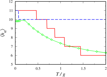
Figure 8: (Color online) Plot of $\langle h_{\alpha}\rangle$ versus $T/g$ in the domain-ground-state region with $J/g=2.5$ and $\alpha$ = 2: MC simulations (diamonds), elastic model with constant (dashed line) and temperature dependent (solid line) stiffness, $k_{0}^{2}\left(\partial^{2}\mathcal{E}_{h}/\partial k_{0}^{2}\right)$ and $k_{0}^{2}\left[\partial^{2}\langle\tilde{\mathcal{H}}_{h}\rangle_{T}/\partial k_{0}^{2}\right]_{\cos}$, respectively (see text).

This procedure produces the dashed line in Fig. 8: For $J/g=2.5$ and $\alpha=2$, the optimal half-period of modulation corresponds the ground-state value, $h_{gs}=11$, for $T<0.07$, while the functional (44) has a minimum in $h=10$ for higher temperatures. All this indicates that the constant decrease of the modulation period observed in the MC simulations is not reproduced just by including thermal fluctuations through a displacement field into the different square-wave profiles and by further minimizing the functional (44) with respect to $h$. Such a failure might be due to the assumption that the stiffness $k_{0}^{2}\left(\partial^{2}\mathcal{E}_{h}/\partial k_{0}^{2}\right)$ remains the same at any temperature. In order to circumvent this limitation, we propose a heuristic extension of our elastic model. Let us first compute the two-point correlations at an infinitesimal temperature $\delta T$:

$$\langle\langle\sigma_{j+r}\sigma_{j}\rangle_{j}\rangle_{\delta T}=\frac{1}{2}\sum_{m=0}^{\infty}\left[a^{2}_{m}\cos\left(k_{m}r\right)e^{-\delta\lambda_{\alpha,m}r}\right]$$ (46)

with $k_{m}=(2m+1)\pi/h$ and $\delta\lambda_{\alpha,m}=k_{m}^{2}\delta T/\left[2k_{0}^{2}\left(\partial^{2}\mathcal{E}_{h}/\partial k_{0}^{2}\right)\right]$. The correlations (46) can be thought of as resulting from a rigid spin profile

$$\sigma_{j}=\sum_{m=0}^{\infty}a_{m}\sin\left(q_{m}j\right)$$ (47)

in which the wave numbers $q_{m}=(2m+1)q_{0}$ are statistically distributed. In particular, if a Lorentzian distribution

$$P(q_{m})=\frac{\delta\lambda_{\alpha,m}}{\pi}\frac{1}{\delta\lambda^{2}_{\alpha,m}+\left(q_{m}-k_{m}\right)^{2}}$$ (48)

is assumed, the corresponding averages – performed after the site average $\langle\dots\rangle_{j}$ – mimic the effect of thermal fluctuations such that Eq. (46) can then be rewritten as

$$\langle\langle\sigma_{j+r}\sigma_{j}\rangle_{j}\rangle_{\delta T} =\langle\langle\sigma_{j+r}\sigma_{j}\rangle_{j}\rangle_{q_{m}}$$

$$=\frac{1}{2}\sum_{m=0}^{\infty}\left[a^{2}_{m}\int_{-\infty}^{+\infty}dq_{m}P(q_{m})\cos\left(q_{m}r\right)\right]\,.$$ (49)

The corresponding energy functional reads

$$\langle\tilde{\mathcal{H}}_{h}\rangle_{\delta T} =\langle\tilde{\mathcal{H}}_{h}\rangle_{q_{m}}=\int_{-\infty}^{+\infty}dq_{m}P(q_{m})$$

$$\qquad\times\left[-NJ\langle\sigma_{j+1}\sigma_{j}\rangle_{j}+N\frac{g}{2}\sum_{r\geq 1}\frac{\langle\sigma_{j+r}\sigma_{j}\rangle_{j}}{r^{\alpha}}\right]$$

$$=\sum_{m=0}^{\infty}\left[a^{2}_{m}\int_{-\infty}^{+\infty}dq_{m}P(q_{m})f_{\alpha}(q_{m})\right]$$ (50)

To the aim of computing the correlation function at an infinitesimally higher temperature, the spin profile (47) can be further perturbed with a displacement field, which brings an increment to the energy functional (50) equal to

$$\langle\Delta\tilde{\mathcal{H}}_{h}\rangle_{q_{m}}=\frac{1}{N}\sum_{q}\sum_{m=0}^{\infty}\left\{a^{2}_{m}\int_{-\infty}^{+\infty}dq_{m}P(q_{m})\right.$$

$$\left.\times q^{2}_{m}\left[\frac{1}{2}f_{\alpha}(q_{m}-q)+\frac{1}{2}f_{\alpha}(q_{m}+q)-f_{\alpha}(q_{m})\right]|\tilde{u}_{q}|^{2}\right\}\,.$$ (51)

By analogy with what done in the previous Section, we perform an expansion for $q\ll k_{0}$ (since $q_{0}$s follow a Lorentzian distribution with maximum in $k_{0}$, $q\ll q_{0}$ as well):

$$\langle\Delta\tilde{\mathcal{H}}_{h}\rangle_{q_{m}} =\frac{1}{N}\sum_{q}\sum_{m=0}^{\infty}\left\{a^{2}_{m}\int_{-\infty}^{+\infty}dq_{m}P(q_{m})\right.$$

$$\qquad\qquad\qquad\qquad\qquad\times\left.q^{2}_{m}\frac{1}{2}\frac{\partial^{2}f_{\alpha}}{\partial q_{m}^{2}}q^{2}|\tilde{u}_{q}|^{2}\right\}\,.$$ (52)

The fact that $q_{m}=(2m+1)q_{0}$ implies $\partial q_{m}/\partial q_{0}=q_{m}/q_{0}$, $\partial^{2}q_{m}/\partial^{2}q_{0}=0$ and consequently

$$\langle\Delta\tilde{\mathcal{H}}_{h}\rangle_{q_{m}}=\frac{1}{N}\sum_{q}\frac{1}{2}\langle q^{2}_{0}\frac{\partial^{2}\tilde{\mathcal{H}}_{h}}{\partial q_{0}^{2}}\rangle_{q_{m}}q^{2}|\tilde{u}_{q}|^{2}\,.$$ (53)

In the present case, the effective stiffness $\langle q^{2}_{0}\left(\partial^{2}\tilde{\mathcal{H}}_{h}/\partial q_{0}^{2}\right)\rangle_{q_{m}}$ has a more complicated dependence on $q_{0}$ with respect to Eq. (35). However, we can simplify its computation significantly with the approximation

$$\langle q^{2}_{0}\frac{\partial^{2}\tilde{\mathcal{H}}_{h}}{\partial q_{0}^{2}}\rangle_{q_{m}}\simeq k_{0}^{2}\frac{\partial^{2}\langle\tilde{\mathcal{H}}_{h}\rangle_{q_{m}}}{\partial k_{0}^{2}}\big{|}_{\cos}=k_{0}^{2}\frac{\partial^{2}\langle\tilde{\mathcal{H}}_{h}\rangle_{\delta T}}{\partial k_{0}^{2}}\big{|}_{\cos}\,,$$ (54)

$\frac{\partial^{2}\langle\tilde{\mathcal{H}}_{h}\rangle_{\delta T}}{\partial k_{0}^{2}}\big{|}_{\cos}$ meaning that the derivative with respect to $k_{0}$ involves only the fluctuating functions, $\cos\left(k_{m}r\right)$. The correlation function at the new temperature ($T=\delta T+\delta T$) is given by

$$\langle\langle\sigma_{j+r}\sigma_{j}\rangle_{j}\rangle_{T}=\frac{1}{2}\sum_{m=0}^{\infty}\left[a^{2}_{m}\int_{-\infty}^{+\infty}dq_{m}P(q_{m})\right.$$

$$\qquad\qquad\qquad\times\left.\cos\left(q_{m}r\right){\rm exp}\left(-\frac{q_{m}^{2}}{2}\frac{\delta T}{k_{0}^{2}\frac{\partial^{2}\langle\tilde{\mathcal{H}}_{h}\rangle_{\delta T}}{\partial k_{0}^{2}}\big{|}_{\cos}}r\right)\right]$$

$$\simeq\frac{1}{2}\sum_{m=0}^{\infty}\left[a^{2}_{m}\int_{-\infty}^{+\infty}dq_{m}P(q_{m})\cos\left(q_{m}r\right)\right.$$

$$\qquad\qquad\qquad\qquad\qquad\times\left.{\rm exp}\left(-\frac{k_{m}^{2}}{2}\frac{\delta T}{k_{0}^{2}\frac{\partial^{2}\langle\tilde{\mathcal{H}}_{h}\rangle_{\delta T}}{\partial k_{0}^{2}}\big{|}_{\cos}}r\right)\right]$$

where in the last passage we have substituted $q_{m}^{2}$ inside the exponential with its maximum $k_{m}^{2}$. Such an approximation allows writing the energy functional at the new temperature again in the form (50), provided that the HWHM of the Lorentzian distribution $P(q_{m})$ is changed into

$$\delta\lambda_{m}=\frac{k_{m}^{2}}{2}\left[\frac{\delta T}{k_{0}^{2}\frac{\partial^{2}\mathcal{E}_{h}}{\partial k_{0}^{2}}}+\frac{\delta T}{k_{0}^{2}\frac{\partial^{2}\langle\tilde{\mathcal{H}}_{h}\rangle_{\delta T}}{\partial k_{0}^{2}}\big{|}_{\cos}}\right]r\,.$$ (56)

The whole process can then be iterated to obtain correlations at any temperature

$$\langle\langle\sigma_{j+r}\sigma_{j}\rangle_{j}\rangle_{T}=\frac{1}{2}\sum_{m=0}^{\infty}\left[a^{2}_{m}\cos\left(k_{m}r\right)e^{-\lambda_{\alpha,m}(T)r}\right]\,,$$ (57)

and the corresponding energy functional

$$\langle\tilde{\mathcal{H}}_{h}\rangle_{T}=\langle\tilde{\mathcal{H}}_{h}\rangle_{q_{m}}=\sum_{m=0}^{\infty}\left[a^{2}_{m}\int_{-\infty}^{+\infty}dq_{m}P(q_{m})f_{\alpha}(q_{m})\right]$$ (58)

with HWHM of $P(q_{m})$ (letting $\delta T\rightarrow dT$) equal to

$$\lambda_{\alpha,m}(T)=k_{m}^{2}\int_{0}^{T}d\lambda_{\alpha,m}=\frac{1}{2}\frac{k_{m}^{2}}{k_{0}^{2}}\int_{0}^{T}\frac{dT}{\frac{\partial^{2}\langle\tilde{\mathcal{H}}_{h}\rangle_{T}}{\partial k_{0}^{2}}\big{|}_{\cos}}\,.$$ (59)

(Remember that the derivative with respect to $k_{0}$ involves only the fluctuating functions, $\cos\left(k_{m}r\right)$, and not the dumping terms). By minimizing numerically the functional (58) with respect to $h$ we obtain the step-like curve in Fig. 8. In this case a decrease with increasing temperature is indeed observed throughout the investigated range. Such a qualitative agreement with MC results suggests that the change in the modulation period and in the effective stiffness, $k_{0}^{2}\left[\partial^{2}\langle\tilde{\mathcal{H}}_{h}\rangle_{T}/\partial k_{0}^{2}\right]_{\cos}$, should be closely related. It is worth remarking that a better agreement is, probably, not to be expected given the expansion for $q\ll k_{0}$ that we performed to pass from (LABEL:DFIF_perturb_energy_4_app_B) to (33) and the further approximations in Eq. (54) and Eq. (LABEL:correlation_q_m_2).

References

• (1) M. Seul, and D. Andelman, Science 267, 476 (1995), and references therein.
• (2) C. B. Muratov, Rev. Mod. E 66, 066108 (2002), and references therein.
• (3) A. Giuliani, J. L. Lebowitz, and E. H. Lieb, Phys. Rev. B 74, 064420 (2006).
• (4) M. Biskup, L. Chayes, and S. A. Kivelson, Comm. Math. Phys. 274, 217 (2007).
• (5) R. Jamei, S. A. Kivelson, and B. Spivak, Phys. Rev. Lett. 94, 056805 (2005).
• (6) D. G. Barci, and D. A. Stariolo, Phys. Rev. Lett. 98, 200604 (2007).
• (7) Z. Nussinov, J. Rudnick, S. A. Kivelson, and L. N. Chayes, Phys. Rev. Lett. 83, 472 (1999).
• (8) Z. Nussinov, arXiv:cond-mat/0506554.
• (9) K. De’Bell, A. B. MacIsaac, and J. P. Whitehead, Rev. Mod. Phys. 72, 225 (2000).
• (10) M. Grousson, G. Tarjus, and P. Viot, Phys. Rev. E 62, 7781 (2000).
• (11) M. Grousson, V. Krakoviack, G. Tarjus, and P. Viot, Phys. Rev. E 66, 026126 (2002).
• (12) M. Grousson, G. Tarjus, and P. Viot, Phys. Rev. E, 64, 036109 (2001).
• (13) S. A. Cannas, D. A. Stariolo, and F. A. Tamarit, Phys. Rev. B 69, 092409 (2004), and references therein.
• (14) A. D. Stoycheva, and S. J. Singer, Phys. Rev. Lett. 84, 4657 (2000).
• (15) A. Kerimov, J. Math. Phys. 40, 4956 (1999).
• (16) A. Giuliani, J. L. Lebowitz, and E. H. Lieb, Phys. Rev. B 76, 184426 (2007).
• (17) X. Chen and Y. Oshita, SIAM J. Math. Anal. 37, 1299 (2005).
• (18) A. Giuliani, J. L. Lebowitz, and E. H. Lieb, Comm. Math. Phys. 286, 163 (2009).
• (19) S. Müller, Calculus Var. Partial Differ. Equ. 1, 169 (1993).
• (20) A. Vindigni, N. Saratz, O. Portmann, D. Pescia, and P. Politi, Phys. Rev. B 77, 092414 (2008).
• (21) O. Portmann, A. Vaterlaus, and D. Pescia, Phys. Rev. Lett. 96, 047212 (2006).
• (22) K. A. Dill, and S. Bromberg, Molecular Driving Forces: Statistical Thermodynamics in Chemistry and Biology, (Garland Science, New York, 2003).
• (23) A. V. Finkelstein, and O. Ptitsyn, Protein Physics (Academic Press, Amsterdam, 2002).
• (24) N. A. Alves, and U. H. E. Hansmann, Phys. Rev. Lett. 84, 1836 (2000), and references therein.
• (25) L. D. Landau, and E. M. Lifshitz, Statistical Physics (Pergamon Press, Oxford, 1980).
• (26) J. Schmalian, and P. G. Wolynes, Phys. Rev. Lett. 85, 836 (2000).
• (27) P. M. Gleiser, F. A. Tamarit, and S. A. Cannas, M. A. Montemurro, Phys. Rev. B 68, 134401 (2003).
• (28) P. M. Gleiser, F. A. Tamarit, and S. A. Cannas, Physica D 168-169, 73 (2002).
• (29) D. A. Stariolo, and S. A. Cannas, Phys. Rev. B 60, 3013 (1999).
• (30) J. H. Toloza, F. A. Tamarit, and S. A. Cannas, Phys. Rev. B 58, R8885 (1998).
• (31) P. M. Chaikin, and T. C. Lubensky, Principles of condensed matter physics (Cambridge University Press, Cambridge, 1995).
• (32) J. Barré, D. Mukamel and S. Ruffo, Phys. Rev. Lett. 87, 030601 (2001).
• (33) J. Barré, F. Bouchet, T. Dauxois, S. Ruffo, J. of Stat. Phys. 119, 677 (2005).
• (34) D. Mukamel, arXiv:0811.3120 [cond-mat.stat-mech].
• (35) Ar. Abanov, V. Kalatsky, V. L. Pokrovsky, and W. M. Saslow, Phys. Rev. B 51, 1023 (1995).
• (36) A. B. Kashuba, and V. L. Pokrovsky, Phys. Rev. B 48, 10335 (1993).
• (37) F. Wegner, Z. Phys. 206, 465 (1967).
• (38) M. E. Fisher, Am. J. Phys. 32, 343 (1964).
• (39) J. A. Krumhansl, J. R. Shriffer, Phys. Rev. B 11, 3535 (1975).
• (40) R. Peierls, Helv. Phys. Acta 7, Suppl. II, 81 (1934).
• (41) S. A. Pighin, and S. A. Cannas, Phys. Rev. B 75, 224433 (2007), and references therein.
• (42) E. Rastelli, S. Regina, and A. Tassi, Phys. Rev. B 76, 054438 (2007).
• (43) E. Ising, Z. Phys. 31, 253 (1925).
• (44) K. Huang, Statistical mechanics (J. Wiley and C., New York, 1987).
• (45) Dynamics and thermodynamics of systems with long-range interactions: theory and experiments, AIP Conference proceedings, edited by A. Campa, A. Giansanti, G. Morigi, and F. S. Labini (Melville, New York, 2008), Vol. 970.
• (46) D. P. Landau, and K. Binder, A Guide to Monte Carlo Simulation in Statistical Physics (Cambridge University Press, Cambridge, 2000).
• (47) S. A. Cannas, C. M. Lapilli, and D. A. Stariolo, Int. J. Mod. Phys. C 15, 115 (2004).
• (48) S. Kirkpatrick, C. D. Gelatt, and M. P. Vecchi, Science 220, 671 (1983).
• (49) K. H. Fischer, and J. A. Hertz, Spin Glasses (Cambridge University Press, 1991).
• (50) Frustrated spin Systems, edited by H. T. Diep (World Scientific, 2004).
• (51) Quantum Annealing and Related Optimization Methods, Lecture Note in Physics, edited by A. Das and B. K. Chakrabarti (Springer, Heidelberg, 2005), Vol. 679.
• (52) E. Luijten and H. W.  J. Bloete, Int. J. Mod. Phys. C 6, 359 (1995).