Multi-fermion interaction models in curved spacetime

Abstract

A model with a scalar type eight-fermion interaction is investigated in curved spacetime. The ground state of the model can be obtained by observing the effective potential. Applying the Riemann normal coordinate expansion, we calculate an effective potential of the model in a weakly curved spacetime. The result is extended to models with multi-fermion interactions. We numerically show the behavior of the effective potential and find the phase structure of the model.

1 Introduction

It is expected that a fundamental theory with a higher symmetry may be realized at high energy scale. The theory is inspected in critical phenomena at early universe. A mechanism to break the symmetry has played a decisive role to construct a theory of particle physics. One of possible mechanisms is found in hadron physics. A composite operator constructed by quark and anti-quark develops a non-vanishing expectation value and the approximate chiral symmetry is broken dynamically. The broken symmetry is restored at high temperature, density and/or strong curvature. These phenomena are understood by non-perturbative dynamics in non-Abelian gauge theories (QCD, SM, GUT, $\cdots$).

A four-fermion interaction model is introduced to particle physics by Nambu and Jona-Lasinio to study low energy phenomena of the strong interaction[1]. The model has a similar apparent symmetry to the low energy limit of QCD. Non-perturbative phenomena in the model can be evaluated trough the expansion in terms of the number of fermion flavors. It can be observed that the chiral symmetry is dynamically broken for a sufficiently strong coupling according to a vacuum condensate of the composite field of fermions. Now some kinds of four-fermion interactions are used to analyze phase transition and critical behavior under extreme conditions.

There are many works to study the curvature induced phase transition in four-fermion interaction models. The pioneering works have been done by Itoyama, Buchbinder and Kirillova in two dimensions.[2, 3] In Refs. [4, 5] and [6], four-fermion interaction models are studied in four, three and arbitral dimensions ($2\leq D<4$) respectively. The phase structure of the model is found in the maximally symmetric spacetime [7, 8], Einstein space [9] and a curved spacetime with a nontrivial topology [10]. For a review, see for example Ref. [11]. The phase structure of the models depends on the coupling constants and the spacetime curvature. The broken chiral symmetry is restored if the spacetime curvature is positive and strong enough. However, the chiral symmetry is always broken down in a negative curvature spacetime even if the four-fermion coupling is small. This is one of the characteristic features in the four-fermion models.

Since the four-fermion interactions are the lowest dimensional operator to describe the fermion self interaction, we often consider only the four-fermion interactions at low energy. However, it is not always valid to neglect higher dimensional operators in the low energy effective models. For example, ’t Hooft introduced a determinantal interactions in a low energy effective model of QCD to deal with the explicit breaking of the $U_{A}(1)$ symmetry [12]. R. Alkofer and I. Zahed considered an eight-fermion interaction to explain the pseudoscalar nonet mass spectrum [13]. An influence of higher derivatives is considered in Ref. [14].

In the present paper we consider higher dimensional scalar type interactions and study the curvature induced chiral symmetry breaking. In Sec.2 we investigate a model with four- and eight-fermion interactions in curved spacetime. Using the auxiliary field method and applying the Riemann normal coordinate expansion, we calculate the effective potential in a weakly curved spacetime. In Sec. 3 we introduce multi-fermion interactions and generalize the auxiliary field method. In some specific cases we show a correspondence with the mean field approximation. In Sec.4 we study the form of the effective potential near the origin. It is shown that the chiral symmetry is always broken in a negative curvature spacetime. In Sec.5 we numerically evaluate the effective potential and show the phase structure of the model with four- and eight-fermion interactions. We discuss the contribution from the higher dimensional operator to the chiral symmetry breaking. Finally we give some concluding remarks.

2 Eight-fermion interaction model in curved spacetime

In this section we introduce a model with scalar type four- and eight-fermion interactions and calculate the effective potential of the model in weakly curved spacetime.

Four-fermion interaction models are often used to study the critical phenomena of dynamical symmetry breaking. The simplest model to induce the dynamical symmetry breaking is Gross-Neveu model[15]. We extend the action of the Gross-Neveu model with an eight-fermion interaction,

$$S = \int d^{4}x\sqrt{-g}\left[\sum_{i=1}^{N}\bar{\psi}_{i}i\gamma^{\mu}(x)\nabla_{\mu}\psi_{i}\right.$$ (1)

$$\left.+\frac{G_{1}}{N}(\sum_{i=1}^{N}\bar{\psi}_{i}\psi_{i})^{2}+\frac{G_{2}}{N}(\sum_{i=1}^{N}\bar{\psi}_{i}\psi_{i})^{4}\right],$$

where the index $i$ shows the flavors of the fermion field $\psi$, $N$ is the number of flavors, $G_{1}$ and $G_{2}$ the coupling constants for the four- and the eight-fermion interactions respectively, $g$ the determinant of the metric tensor, $\gamma^{\mu}(x)$ the Dirac matrix in curved spacetime and $\nabla_{\mu}\psi$ the covariant derivative of the fermion field $\psi$.

The action (1) is symmetric under the discrete chiral transformations,

$$\psi_{i}\rightarrow\gamma_{5}\psi_{i},$$ (2)

This chiral symmetry prevents the action from having mass term.

The action is also invariant under a global flavor transformation,

$$\psi_{i}\rightarrow\left(\exp(i\sum_{a}\theta_{a}T_{a})\right)_{ij}\psi_{j},$$ (3)

where $T_{a}$ are generators of the flavor $SU(N)$ symmetry. The flavor symmetry allows us to work in a scheme of the $1/N$ expansion. Below we neglect the flavor index for simplicity.

For practical calculations it is more convenient to introduce auxiliary fields $\sigma_{1}$ and $\sigma_{2}$ and rewrite the action in the following form,

$$S_{\sigma}=\int d^{4}x\sqrt{-g}\left[\bar{\psi}\left(i\gamma^{\mu}(x)\nabla_{\mu}-\sigma\right)\psi-\frac{N\sigma_{1}^{2}}{4G_{1}}-\frac{N\sigma_{2}^{2}}{4G_{2}}\right],$$ (4)

where $\sigma$ is defined by

$$\sigma:=\sigma_{1}\sqrt{1-\frac{N\sigma_{2}}{G_{1}}}.$$ (5)

The equations of motion for the auxiliary fields are given by

$$\sigma_{1} = -\frac{2G_{1}}{N}\sqrt{1-\frac{N\sigma_{2}}{G_{1}}}\bar{\psi}\psi,$$ (6)

$$\sigma_{2} = -\frac{2G_{2}}{N}(\bar{\psi}\psi)^{2}\;.$$ (7)

Substituting these equations of motion into the action (4), we obtain the original action (1).

If the non-vanishing expectation value is assigned to $\sigma$, a mass term for the fermion filed $\psi$ is dynamically generated and the chiral symmetry is eventually broken. To study the phase structure we want to find the ground state of the model. In the present paper we assume that the spacetime curved slowly and neglect terms involving derivatives of the metric tensor higher than second order. We also restrict ourselves to the static and homogeneous spacetime. In this case we can assume that the expectation values for $\sigma_{1}$ and $\sigma_{2}$ are constant.

The energy density under the constant background $\sigma_{1}$ and $\sigma_{2}$ is given by the effective potential. At the large $N$ limit the effective potential $V$ is obtained by evaluating vacuum bubble diagrams,

$$V(\sigma_{1},\sigma_{2})=\frac{\sigma_{1}^{2}}{4G_{1}}+\frac{\sigma_{2}^{2}}{4G_{2}}+v(\sigma),$$ (8)

where we drop the over all factor $N$ and $v(\sigma)$ is given by

$$v(\sigma):=\frac{i}{N}\mbox{Tr}\ln\left<x|\left[i\gamma^{\mu}(x)\nabla_{\mu}-\sigma\right]|x\right>,$$ (9)

where ”Tr” denotes trace with respect to flavor, spinor indices and spacetime coordinate. The ground state should minimize this effective potential.

Since the four- and the eight fermion interactions are nonrenormalizable, above $v(\sigma)$ is divergent. To obtain the finite result we regularize the divergent integral by the cut-off method. After performing the Fourier transformation and the Wick rotation, we introduce the four-momentum cut-off, $\Lambda$. Applying the Riemann normal coordinate expansion, we expand the effective potential and find

$$v(\sigma) = -\frac{1}{(4\pi)^{2}}\left[\sigma^{2}\Lambda^{2}+\Lambda^{4}\ln\left(1+\frac{\sigma^{2}}{\Lambda^{2}}\right)-\sigma^{4}\ln\left(1+\frac{\Lambda^{2}}{\sigma^{2}}\right)\right]$$ (10)

$$-\frac{1}{(4\pi)^{2}}\frac{R}{6}\left[-\sigma^{2}\ln\left(1+\frac{\Lambda^{2}}{\sigma^{2}}\right)+\frac{\Lambda^{2}\sigma^{2}}{\Lambda^{2}+\sigma^{2}}\right]+O(R_{;\mu},R^{2}).$$

We keep only terms independent of the curvature $R$ and terms linear in $R$. To determine the ground state we can freely normalize the effective potential. Here the effective potential is normalized so that $V(0,0)=0$.

The necessary condition for the minimum of the effective potential is given by the gap equations,

$$\frac{\partial V(\sigma_{1},\sigma_{2})}{\partial\sigma_{1}}=\frac{\sigma_{1}}{2G_{1}}+\frac{dv(\sigma)}{d\sigma}\frac{\partial\sigma}{\partial\sigma_{1}}=0,$$ (11)

and

$$\frac{\partial V(\sigma_{1},\sigma_{2})}{\partial\sigma_{2}}=\frac{\sigma_{2}}{2G_{2}}+\frac{dv(\sigma)}{d\sigma}\frac{\partial\sigma}{\partial\sigma_{2}}=0,$$ (12)

with

$$\frac{\partial\sigma}{\partial\sigma_{1}} = \sqrt{1-\frac{N\sigma_{2}}{G_{1}}}\;,\;\;\frac{\partial\sigma}{\partial\sigma_{2}}=-\frac{N\sigma_{1}}{2G_{1}\sqrt{1-\frac{\displaystyle N\sigma_{2}}{\displaystyle G_{1}}}},$$

$$\frac{dv(\sigma)}{d\sigma} = -\frac{\sigma}{4\pi^{2}}\left[\Lambda^{2}-\sigma^{2}\ln\left(1+\frac{\Lambda^{2}}{\sigma^{2}}\right)\right]$$ (13)

$$-\frac{\sigma}{48\pi^{2}}R\left[-\ln\left(1+\frac{\Lambda^{2}}{\sigma^{2}}\right)+\frac{\Lambda^{2}}{\Lambda^{2}+\sigma^{2}}+\frac{\Lambda^{4}}{(\Lambda^{2}+\sigma^{2})^{2}}\right].$$

Under the ground state the expectation values for $\sigma_{1}$ and $\sigma_{2}$ satisfy these gap equations. From the gap equations (11) and (12) we find the following conditions for non-vanishing expectation values of $\sigma_{1}$ and $\sigma_{2}$.

$$\langle\sigma_{1}\rangle^{2}=\frac{2G_{1}}{G_{2}}\langle\sigma_{2}\rangle\left(\langle\sigma_{2}\rangle-\frac{G_{1}}{N}\right),$$ (14)

or

$$\frac{1}{2G_{1}}-\frac{1}{4\pi^{2}}\left[\Lambda^{2}-\langle\sigma_{1}\rangle^{2}\ln\left(1+\frac{\Lambda^{2}}{\langle\sigma_{1}\rangle^{2}}\right)\right]$$

$$-\frac{R}{48\pi^{2}}\left[-\ln\left(1+\frac{\Lambda^{2}}{\langle\sigma_{1}\rangle^{2}}\right)+\frac{\Lambda^{2}}{\Lambda^{2}+\langle\sigma_{1}\rangle^{2}}+\frac{\Lambda^{4}}{(\Lambda^{2}+\langle\sigma_{1}\rangle^{2})^{2}}\right]=0,$$

$$\langle\sigma_{2}\rangle=0.$$ (15)

One of the conditions (14) and (15) should be satisfied at the minimum of the effective potential. In the former case the expectation values for $\sigma_{1}$ and $\sigma_{2}$ are on a hyperbolic curve for a positive $G_{1}G_{2}$ or on an ellipse for a negative $G_{1}G_{2}$. The latter condition is the same as that in the four-fermion interaction model and the eight-fermion interaction has nothing to do with the ground state.

At the ground state the expectation values obey the classical equations of motion. Substituting Eqs.(6) and (7) into the conditions (14) or (15), we find one of the following relationships,

$$\left<(\bar{\psi}\psi)^{2}\right>=\left<(\bar{\psi}\psi)\right>^{2},\mbox{ or }\left<(\bar{\psi}\psi)^{2}\right>=0.$$ (16)

These relationships mean that our result at the leading order of the $1/N$ expansion coincides with the one in the mean field approximation except for the case, $\left<(\bar{\psi}\psi)^{2}\right>=0$.

We numerically evaluate the effective potential (8) and show the phase structure of the model in Sec.4.

3 Multi-fermion interactions

The results in the previous section can be extended more general cases. The extension of the model is not unique. Here we assume that vector, tensor type interactions and interactions with derivative operator do not develop expectation values at the ground state and contribution to the phase structure is negligible. We consider models with only scalar-type multi-fermion interactions and calculate the gap equation.

We start from the action defined by

$$S=\int d^{4}x\sqrt{-g}\left[\bar{\psi}i\gamma^{\mu}(x)\nabla_{\mu}\psi+\sum^{n}_{k=1}G_{k}(\bar{\psi}\psi)^{2k}\right].$$ (17)

This action is invariant under the discrete chiral transformation (2) and the global flavor transformation (3).

According to the functional integral formalism, the generating functional is given by

$$Z=\int{\cal D}\tilde{\psi}{\cal D}\tilde{\bar{\psi}}e^{iS},$$ (18)

where we set the path-integral measure, $\tilde{\psi}\equiv\sqrt[4]{-g}\psi$ and $\tilde{\bar{\psi}}\equiv\sqrt[4]{-g}\bar{\psi}$, to keep the general covariance.

We consider a Gaussian integral

$$C := \int\prod_{k=1}^{n}{\cal D}\sigma_{k}$$ (19)

$$\times\exp\left\{i\int d^{4}x\sqrt{-g}\sum_{l=1}^{n}\left[-\frac{N}{4G_{l}}\left(\sigma_{l}+\frac{1}{N}\sum^{l}_{m=1}a_{lm}(\bar{\psi}\psi)^{m}\right)^{2}\right]\right\},$$

and inserts it in the right-hand side of Eq.(18). Thus the generating functional (18) is rewritten as

$$Z=\frac{1}{C}\int{\cal D}\tilde{\psi}{\cal D}\tilde{\bar{\psi}}\prod_{k=1}^{n}{\cal D}\sigma_{k}e^{iS_{y}},$$ (20)

where the action $S_{y}$ is given by

$$S_{y} = \int d^{4}x\sqrt{-g}\left[\bar{\psi}i\gamma^{\mu}\nabla_{\mu}\psi+\sum_{k=1}^{n}\frac{G_{k}}{N}(\bar{\psi}\psi)^{2k}\right.$$ (21)

$$\left.-\sum_{k=1}^{n}\frac{N}{4G_{k}}\left(\sigma_{k}+\frac{1}{N}\sum_{l=1}^{k}a_{kl}(\bar{\psi}\psi)^{l}\right)^{2}\right].$$

Since the number of arbitrary parameters, $a_{kl}$, is $n(n+1)/2$, we can choose $a_{kl}=a_{kl}(\sigma_{k+1},\sigma_{k+2},\cdots,\sigma_{n})$ to satisfy

$$\sum_{k=1}^{n}\frac{N}{4G_{k}}\left(\sigma_{k}+\frac{1}{N}\sum_{l=1}^{k}a_{kl}(\bar{\psi}\psi)^{l}\right)^{2}$$

$$=f(\sigma)\bar{\psi}\psi+\sum_{k=1}^{n}\left(\frac{G_{k}}{N}(\bar{\psi}\psi)^{2k}+\frac{N}{4G_{k}}\sigma_{k}^{2}\right),$$ (22)

where $f(\sigma)$ is a function of $\sigma_{k}$ $(k=1,2,\cdots,n)$. Therefore the multi-fermion interaction terms in Eq.(21) are canceled out and the action $S_{y}$ reduces to

$$S_{y}=\int d^{4}x\sqrt{-g}\left[\bar{\psi}(i\gamma^{\mu}\nabla_{\mu}-f(\sigma))\psi-\sum_{k=1}^{n}\frac{N}{4G_{k}}{\sigma_{k}}^{2}\right].$$ (23)

Applying the similar method mentioned in the previous section, we obtain the effective potential

$$V(\sigma_{1},\cdots,\sigma_{n})=\sum_{k=1}^{n}\frac{{\sigma_{k}}^{2}}{4G_{k}}+v(f(\sigma)),$$ (24)

where $v$ is defined in Eq.(10).

We calculate the explicit expression of $f(\sigma)$ for some cases. For $n=2$ it is easy to reproduce the result in Eq. (5). As another simple case, we consider the action,

$$S=\int d^{4}x\sqrt{-g}\left[\bar{\psi}i\gamma^{\mu}(x)\nabla_{\mu}\psi+\sum^{n}_{k=1}\frac{g_{k}}{N}(\bar{\psi}\psi)^{2^{k}}\right].$$ (25)

In this case the function $f(\sigma)$ is given by the following induction series,

$$f(\sigma):=\sigma_{1}^{\prime},\sigma_{k}^{\prime}:=\sigma_{k}\sqrt{1-\frac{N\sigma_{k+1}^{\prime}}{g_{k}}}\;\;(k=1,\cdots n),\sigma_{n+1}^{\prime}:=0.$$ (26)

It is straightforward to show that above $f(\sigma)$ satisfies,

$$\sum_{k=1}^{n}\frac{N}{4g_{k}}\left(\sigma_{k}+\frac{1}{N}a_{k}(\bar{\psi}\psi)^{2^{k-1}}\right)^{2}$$

$$=f(\sigma)\bar{\psi}\psi+\sum_{k=1}^{n}\left(\frac{g_{k}}{N}(\bar{\psi}\psi)^{2^{k}}+\frac{N}{4g_{k}}\sigma_{k}^{2}\right),$$ (27)

with

$$a_{k}:=2g_{k}\sqrt{1-\frac{N\sigma_{k+1}^{\prime}}{g_{k}}},a_{n}:=-2g_{n}.$$ (28)

for $k=1,\cdots n$. It is a sufficient condition for Eq.(22). Hence, the action (25) is simplifies to

$$S_{y}=\int d^{4}x\sqrt{-g}\left[\bar{\psi}(i\gamma^{\mu}\nabla_{\mu}-f(\sigma))\psi-\sum_{k=1}^{n}\frac{N}{4g_{k}}{\sigma_{k}}^{2}\right].$$ (29)

Since the effective potential has the same form with Eq.(24), the gap equations for the action (29) are given by

$$\frac{\partial V(\sigma_{1},\cdots,\sigma_{n})}{\partial\sigma_{k}}=\frac{\sigma_{k}}{2g_{k}}+\frac{dv(f(\sigma))}{df(\sigma)}\frac{\partial f(\sigma)}{\partial\sigma_{k}}=0\;,\;\;(k=1,2,\cdots,n)$$ (30)

Differentiating $f(\sigma)$ with respect to $\sigma_{k}$, we get

$$\frac{\partial f(\sigma)}{\partial\sigma_{k}}=\frac{\partial\sigma}{\partial\sigma_{1}^{\prime}}\frac{\partial\sigma_{1}^{\prime}}{\partial\sigma_{2}^{\prime}}\cdots\frac{\partial\sigma_{k-1}^{\prime}}{\partial\sigma_{k}^{\prime}}\frac{\partial\sigma_{k}^{\prime}}{\partial\sigma_{k}}=\prod_{i=1}^{k-1}\sigma_{i}\frac{-N/g_{i}}{2\sqrt{1-\frac{N\sigma_{i+1}^{\prime}}{g_{i}}}}\sqrt{1-\frac{N\sigma_{k+1}^{\prime}}{g_{k}}},$$ (31)

for $k=1,2,\cdots,n$. We calculate the ratio between $(k-1)$-th and $k$-th equations of (30),

$$\frac{g_{k-1}}{g_{k}}\frac{\sigma_{k}}{\sigma_{k-1}}=\left(\frac{\partial f(\sigma)}{\partial\sigma_{k}}\right)\bigg{/}\left(\frac{\partial f(\sigma)}{\partial\sigma_{k-1}}\right).$$ (32)

Substituting the Eq.(31) into Eq.(32), we obtain the following configuration for $\sigma_{k}$ at the ground state,

$$\frac{\sigma_{k}}{2g_{k}}\frac{1}{\sqrt{1-\frac{N\sigma_{k+1}^{\prime}}{g_{k}}}}=-\frac{N\sigma_{k-1}^{2}}{4g_{k-1}^{2}}\frac{1}{1-\frac{N\sigma_{k}^{\prime}}{g_{k-1}}},\mbox{ or }\sigma_{k}=0.$$ (33)

For the action (29) the equations of motion are given by

$$\sigma_{k}=-\frac{2g_{k}}{N}\sqrt{1-\frac{N\sigma_{k+1}^{\prime}}{g_{k}}}(\bar{\psi}\psi)^{2^{k-1}}.$$ (34)

At the ground state it is valid to insert Eq.(34) into Eq.(33). Then we eliminate $\sigma_{k-1}$, $\sigma_{k}$, $\sigma_{k}^{\prime}$ and $\sigma_{k+1}^{\prime}$ from both the sides in Eq.(33) and find following relationships between expectation values,

$$\langle(\bar{\psi}\psi)^{2^{k}}\rangle=\langle\bar{\psi}\psi\rangle^{2^{k}},\mbox{ and }\langle(\bar{\psi}\psi)^{2^{k^{\prime}}}\rangle=0.$$ (35)

for $k=1,2,\cdots,k^{\prime}$ and $k^{\prime}\in\{2,\cdots,n+1\}$. The number $k^{\prime}$ depends on details of the effective potential and is fixed by observing the minimum of that. Therefore the solution of the gap equations (30) are equivalent to the ones obtained by the mean fields approximation for $k<k^{\prime}$.

4 Chiral symmetry breaking in a negative curvature spacetime

In a scalar type four-fermion interaction model the chiral symmetry is always broken in a negative curvature spacetime. Here we study the behavior of the effective potential near the origin and show the chiral symmetry breaking for $R<0$ in a multi-fermion interaction model.

First we consider the eight-fermion interaction model (1). To obtain a precise form of the effective potential we evaluate the curvature of the effective potential at the limit $\sigma_{1}\rightarrow 0$ and $\sigma_{2}\rightarrow 0$. Differentiating the effective potential (8) twice and using the condition (22), we get

$$\frac{\partial^{2}V}{\partial\sigma_{1}^{2}}=\frac{1}{2G_{1}}+\left(1-\frac{N\sigma_{2}}{G_{1}}\right)\frac{d^{2}v}{d\sigma^{2}},$$ (36)

and

$$\frac{\partial^{2}V}{\partial\sigma_{2}^{2}}=\frac{1}{2G_{2}}-\frac{N\sigma_{2}}{2G_{2}}\left(\frac{1}{\sigma}\frac{dv}{d\sigma}+\frac{d^{2}v}{d\sigma^{2}}\right).$$ (37)

For a large $\sigma_{i}$ the effective potential (8) is almost proportional to $\sigma_{i}^{2}$. Thus the potential has a stable minimum. If $\partial^{2}V/\partial\sigma_{1}^{2}$ or $\partial^{2}V/\partial\sigma_{1}^{2}$ is negative at the origin, the effective potential is unstable and the chiral symmetry has to be broken. Taking the limit $\sigma_{1}\rightarrow 0$ and $\sigma_{2}\rightarrow 0$, we obtain,

$$\frac{\partial^{2}V}{\partial\sigma_{1}^{2}}\rightarrow\lim_{\sigma\rightarrow 0}\left[\frac{1}{2G_{1}}-\frac{\Lambda^{2}}{4\pi^{2}}+\frac{R}{4\pi^{2}}\left(\mbox{ln}\left(1+\frac{\Lambda^{2}}{\sigma^{2}}\right)-2\right)\right],$$ (38)

and

$$\frac{\partial^{2}V}{\partial\sigma_{2}^{2}}\rightarrow\frac{1}{2G_{2}}.$$ (39)

The right-hand side in Eq.(38) is always negative for $R<0$. It implies that the auxiliary fields, $\sigma_{1}$ and $\sigma_{2}$, develops non-vanishing values at the minimum of the effective potential. Thus only the broken phase realizes in a negative curvature spacetime.

Next we consider the multi-fermion interaction model (17). Differentiating both the sides of Eq.(22) in terms of $\sigma_{1}$, we obtain

$$\frac{\partial f(\sigma)}{\partial\sigma_{1}}=\frac{1}{2G_{1}}a_{11}(\sigma_{2},\sigma_{3},\cdots,\sigma_{n}).$$ (40)

It should be noted that that the function $a_{11}$ does not depend on $\sigma_{1}$ by definition. Using the condition (40), we differentiate the effective potential (24) twice in terms of $\sigma_{1}$ and get

$$\frac{\partial^{2}V}{\partial{\sigma_{1}}^{2}}=\frac{1}{2G_{1}}+\frac{{a_{11}}^{2}}{4{G_{1}}^{2}}\frac{d^{2}v}{d\sigma^{2}}.$$ (41)

To find the behavior of the effective potential near the origin, we take the limit $\sigma_{2},\sigma_{3},\cdots,\sigma_{n}\rightarrow 0$. At the limit Eq.(22) we obtain,

$$a_{11}(\sigma_{2},\sigma_{3},\cdots,\sigma_{n}\rightarrow 0)=2G_{1}.$$ (42)

Taking the same limit in Eq.(41) and substituting Eq.(42), we obtain Eq.(38) again. According to the same argument as the eight-fermion interaction model at least one of the auxiliary fields, $\sigma_{1}$, develops a non-vanishing value at the minimum of the effective potential. Therefore we conclude that only the broken phase realizes for the scalar type multi-fermion interaction models in a negative curvature spacetime.

5 Numerical analysis of the phase structures

Here we study the contribution from higher dimensional operators to chiral symmetry breaking in curved spacetime. We consider the model with four- and eight-fermion interactions and numerically evaluate the effective potential (8) with (10). We normalize the mass scale by the cut-off scale $\Lambda$. The auxiliary field $\sigma$ plays a role as an order parameter for the chiral symmetry breaking.

We start to calculate the effective potential with fixed coupling constants $G_{1}$ and $G_{2}$. For $G_{2}=0$ the model contains only the four-fermion interaction. In this case the chiral symmetry is broken down for $G_{1}\Lambda^{2}>2\pi^{2}\equiv G^{(R=0)}_{1cr}$ in Mikowski spacetime, i.e. R=0. In a negative curvature spacetime we observe only the broken phase.[4]

For a model with a finite $G_{2}$ we numerically evaluate the effective potential under the constraints (14) and (15). We observe that the minimum of the effective potential satisfies the constraint (14) in all cases we consider here. Therefore we only show the results under the constraint (14) below.

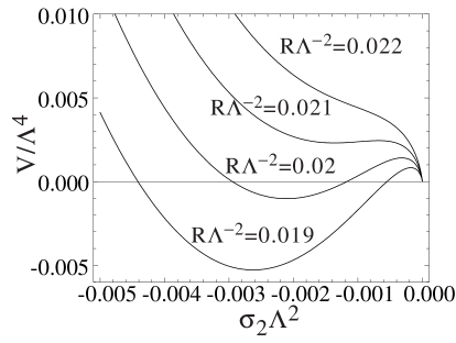
Figure 1: Behavior of the effective potential (8) for $G_{1}\Lambda^{2}=20$ and $G_{2}\Lambda^{8}=1000$.

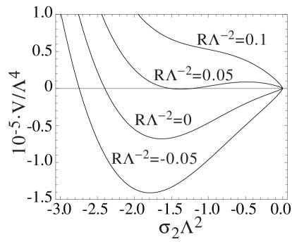
Figure 2: Behavior of the effective potential (8) for $G_{1}\Lambda^{2}=20$ and $G_{2}\Lambda^{8}=8500$.

First we consider the model with a four-fermion coupling, $G_{1}(>G^{(R=0)}_{1cr})$, larger than the critical one for $R=0$ and $G_{2}=0$. In Figs.2 and 2 we draw the behavior of the effective potential as a function of $\sigma_{2}$ for $G_{1}\Lambda^{2}=20$, $G_{2}\Lambda^{8}=1000$ and $G_{1}\Lambda^{2}=20$, $G_{2}\Lambda^{8}=8500$ respectively. In Fig.2 the chiral symmetry is broken for a negative curvature and is restored through the first order phase transition at $R=R_{cr}$, as the curvature increases. Then the symmetric phase is realized for $R>R_{cr}$. In Fig.2 we plot the effective potential for a larger eight-fermion coupling, $G_{2}$. As is seen in the figure, the broken chiral symmetry is restored through the first order phase transition. The critical curvature for $G_{2}\Lambda^{8}=8500$ is larger than that for $G_{2}\Lambda^{8}=1000$. Thus the chiral symmetry breaking is enhanced by the eight-fermion interaction.

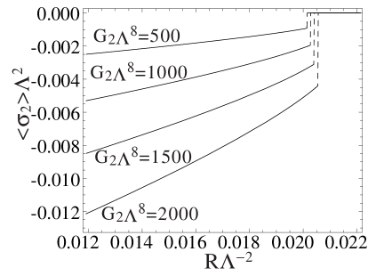
Figure 3: Behavior of the dynamically generated fermion mass for $G_{1}\Lambda^{2}=20$ and $G_{2}\Lambda^{8}=500\sim 2000$.

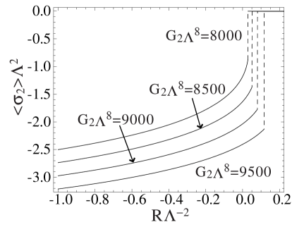
Figure 4: Behavior of the dynamically generated fermion mass for $G_{1}\Lambda^{2}=20$ and $G_{2}\Lambda^{8}=8000\sim 9500$.

Observing the minimum of the effective potential, we obtain the expectation value $\langle\sigma_{2}\rangle$ at the ground state. The expectation value satisfies the gap equations. A non-vanishing $\langle\sigma_{1}\rangle$ is obtained for a non-vanishing and a negative $\langle\sigma_{2}\rangle$ from the constraint (14). It implies a non-vanishing $\langle\sigma\rangle$ which corresponds to the dynamically generated fermion mass. Therefore the chiral symmetry is broken down for a non-vanishing and a negative $\langle\sigma_{2}\rangle$. On the other hand the expectation value $\langle\sigma\rangle$ is vanish for $\langle\sigma_{2}\rangle=0$. In this case the dynamical fermion mass is not generated and the chiral symmetry is guaranteed. Therefore we can inspect the chiral symmetry breaking by the expectation value $\langle\sigma_{2}\rangle$.

In Figs.4 and 4 we draw the expectation value $\langle\sigma_{2}\rangle$ at $G_{1}\Lambda^{2}=20$ as a function of the spacetime curvature, $R$. It is clearly seen that the behavior of each lines are consistent with Figs.2 and 2. The expectation value develops a non-vanishing value for a smaller $R$ and disappears, as the curvature increases. We observe a mass gap in Figs.4 and 4 which reflects the nature of the first order phase transition.

Next we evaluate the model with a four-fermion coupling, $G_{1}(<G^{(R=0)}_{1cr})$, smaller than the critical one for $R=0$ and $G_{2}=0$. An interesting behavior is found for a smaller $G_{1}\Lambda^{2}$. At a glance we may observe a symmetric phase even for a negative curvature spacetime at $G_{1}\Lambda^{2}=15$ in Fig.6.

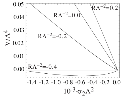
Figure 5: Behavior of the effective potential (8) for $G_{1}\Lambda^{2}=15$ and $G_{2}\Lambda^{8}=8500$.

Figure 6: Behavior of the dynamically generated fermion mass for $G_{1}\Lambda^{2}=15$.

To find the precise behavior of the effective potential we solve the gap equation. In Fig.6 we plot the solution of the gap equation as a function of the curvature. We observe that the expectation value, $\langle\sigma_{2}\rangle$, smoothly disappears as the curvature increases. The transition from the broken phase to the symmetric phase is crossover. Therefore it is difficult to find the critical curvature of these figures. As is shown in Sec.4, the expectation value $\langle\sigma_{2}\rangle$ develops a non-vanishing value and the chiral symmetry is always broken for $R<0$.

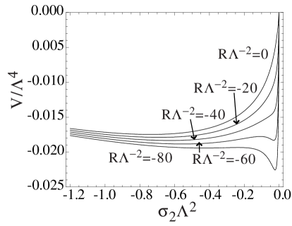
Figure 7: Behavior of the effective potential (8) for $G_{1}\Lambda^{2}=1000$ and $G_{2}\Lambda^{8}=20000$.

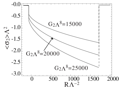
Figure 8: Behavior of the dynamically generated fermion mass for $G_{1}\Lambda^{2}=1000$.

We also consider much larger $G_{1}\Lambda^{2}$. In Fig.8 the effective potential is drawn for $G_{1}\Lambda^{2}=1000$ and $G_{2}\Lambda^{8}=20000$, although the coupling constant $G_{1}$ seems to be too large as a realistic model. It should be noted that we do not use a perturbative expansion in terms of the coupling constant. We observe four extrema at $R/\Lambda^{2}=-60$. As is shown in Fig.8, we find the two kinds of the gaps for $\langle\sigma_{2}\rangle$ at a negative $R$ and a positive $R$. As increasing the curvature, $R$, the chiral symmetry breaking is much enhanced at the gap with a negative $R$ and the broken chiral symmetry is restored through the first order phase transition at the gap with a positive $R$. The gaps appear at a large curvature $|R/(\Lambda^{2})|>1$. Since we work in the Riemann normal coordinate expansion and keep only terms up to linear in $R$, we may spoil the validity of the expansion. These types of the phase transition in Figs. 8 and 8 may be modified by a higher order correction about $R$.

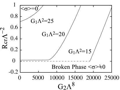
Figure 9: Phase diagram of the eight-fermion interaction model (1) for $G_{1}\Lambda^{2}=15,20$ and $25$.

By observing the behavior of $\langle\sigma_{2}\rangle$, we obtain the phase boundary which separates the chiral symmetric and the broken phases. The boundary curves are shown in Fig.9. Below the lines the chiral symmetry is broken. The first order phase transition is shown by solid lines. The crossover boundary is drown by dashed lines. We find that the chiral symmetry is broken down for an eight-fermion coupling large enough. In the case of the crossover the critical value of the curvature, $R_{\mbox{cr}}$, is almost independent on the eight-fermion coupling, $G_{2}$. If the phase transition is of the first order, the chiral symmetry breaking is enhanced for a larger eight-fermion coupling $G_{2}$.

In this section we confine our selves in the eight-fermion interaction model and numerically evaluate the effective potential and solve the gap equation. It is possible to apply the procedure used here to the multi-fermion interaction models. Since the multi-fermion interaction models have more parameters, we expect that a more complex phase structure is realizes. Before analyze the phase structure more general models with many parameters, it is better to fix the physical phenomena to apply the model and reduce the parameters.

6 Conclusions

We have considered the multi-fermion interaction models as effective models to describe dynamical symmetry breaking at high energy scale and investigated the phase structure in weakly curved spacetime. Applying the Riemann normal coordinate expansion, we have obtained the explicit expression for the effective potential in the leading order of the $1/N$ expansion. One of the solutions of the gap equation coincides with that in the mean field approximation.

To inspect the existence of a non-trivial ground state we have analytically evaluated the second derivative of the effective potential at the trivial solution of the gap equation, $\sigma_{1}=\sigma_{2}=0$. The result is always negative for $R<0$. It implies that the state with $\sigma_{1}=\sigma_{2}=0$ is unstable. Thus only the broken phase can be realized in a negative curvature spacetime. We conclude that the chiral symmetry is always broken in a negative curvature spacetime at the large $N$ limit . It is one of the characteristic features of the multi-fermion interaction model.

We have numerically evaluated details of the phase structure for the eight-fermion interaction model. The broken chiral symmetry was restored at a certain critical curvature, $R_{cr}(\geq 0)$. The contribution of the eight-fermion coupling enhances the chiral symmetry breaking. For a small four-fermion coupling, $G_{1}<G^{(R=0)}_{1cr}$, we observe the crossover behavior, i.e. the non-vanishing expectation value, $\langle\sigma\rangle$, smoothly disappears, as the curvature $R$ increases. For $G_{1}>G^{(R=0)}_{1cr}$ the mass gap appears for the solution of the gap equation and only the first order phase transition realized. We found the phase boundary dividing the symmetric phase and the broken phase. There is no symmetric phase for a negative $R$, as is shown analytically.

We also apply our result to a strongly curve spacetime, though we may spoil the validity of the weak curvature expansion. (For the four-fermion interaction model the validity of the weak curvature expansion in the strongly curved spacetime is discussed in Ref.[6] .) A more complex phase structure is found in this case. We have observed two local minima for the effective potential and two kinds of mass gap for a negative and a large positive curvature.

We are interested in applying our results to critical phenomena in the early universe. A supersymmetric extension of the four-fermion interaction model is discussed in Ref.BIO. A contribution from supersymmetric partners may play an important role at high energy scale. We will continue our work further and hope to report on these problems.

References

References

- [1] Y. Nambu and G. Jona-Lasinio, Phys. Rev. 124 (1961) 246.
- [2] H. Itoyama, Prog. Theor. Phys. 64 (1980) 1886.
- [3] I. L. Buchbinder and E. N. Kirillova, Int. J. of Mod. Phys. A4 (1989) 143.
- [4] T. Inagaki, T. Muta and S. D. Odintsov, Mod. Phys. Lett. A8 (1993) 2117.
- [5] E. Elizalde, S. D. Odintsov and Yu. I. Shil’nov, Mod. Phys. Lett. A9 (1994) 913.
- [6] T. Inagaki, Int. J. of Mod. Phys. A11 (1996) 4561.
- [7] T. Inagaki, S. Mukaigawa, T. Muta, Phys. Rev. D52 (1995) 4267.
- [8] E. Elizalde, S. Leseduarte, S. D. Odintsov and Yu. I. Shilnov, Phys. Rev. D53 (1996) 1917.
- [9] K. Ishikawa, T. Inagaki, T. Muta, Mod. Phys. Lett. A11 (1996) 939.
- [10] E. Elizalde, S. Leseduarte and S. D. Odintsov, Phys. Rev. D49 (1994) 5551.
- [11] T. Inagaki, T. Muta and S. D. Odintsov, Prog. Theor. Phys. Suppl. 127 (1997) 93.
- [12] G. ’t Hooft, Phys. Rev. D14 (1976) 3432; D18 (1978) 2199 (E); Phys. Rep. 142 (1986) 357.
- [13] R. Alkofer and I. Zahed, Phys. Lett. B 238 (1990) 149.
- [14] E. Elizalde, S. Leseduarte and S. D. Odintsov, Phys. Lett. B347 (1995) 33.
- [15] D. J. Gross and A. Neveu, Phys. Rev. D10 (1974) 3235.
- [16] I. L. Buchbinder, T. Inagaki and S. D. Odintsov, Mod. Phys. Lett. A12 (1997) 2271.