Quantum correlations of twophoton polarization states in the parametric down-conversion process

Abstract

We consider correlation properties of twophoton polarization states in the parametric down-conversion process. In our description of polarization states we take into account the simultaneous presence of colored and white noise in the density matrix. Within the considered model we study the dependence of the von Neumann entropy on the noise amount in the system and derive the separability condition for the density matrix of twophoton polarization state, using Perec-Horodecki criterion and majorization criterion. Then the dependence of the Bell operator (in CHSH form) on noise is studied. As a result, we give a condition for determining the presence of quantum correlation states in experimental measurements of the Bell operator. Finally, we compare our calculations with experimental data [4] and give a noise amount estimation in the photon polarization state considered there.

1 Introduction

In 1982 Aspect’s group (Alain Aspect et. al. [1]) performed a verification experiment for possible violation of Bell’s inequalities in Clauser-Horne-Shimony-Holt (CHSH) form [2], where a correlation measurement of twophoton polarization states was provided. Experimental data gave Bell’s inequality violation by five standard deviations. Measurement results corresponded well with predictions of quantum mechanics. Numerous later experiments showed that their results are in agreement with the quantum mechanical description of nature.

Thus, specific quantum correlations obtained the status of reality, and entangled states, which provide such correlations, became an object of intensive research. It turned out that entanglement can play in essence the role of a new resource in such scientific areas as quantum cryptography, quantum teleportation, quantum communication and quantum computation. This became a great stimulus for researching methods of creating, accumulating, distributing and broadcasting this resource.

One of the most important questions in the considered topic concerns methods of identifying the presence of entanglement in one or another realistic quantum mechanical state. Since entangled states violate Bell’s inequalities, the violation of Bell’s inequalities can be a basic tool to detect entanglement. In realistic applications pure entangled states become mixed states due to different types of noise. Thus a question about robustness of Bell’s inequalities violation against the noise arises. In other words, one wants to know, under what proportion of an entangled state and noise in a realistic mixed state the presence of entanglement can be discovered.

The most reliable source of two-party entanglement are polarization-entangled photons created by the parametric down-conversion process (PDC) [3].

2 Noise-present entanglement detection

In 2006 a paper by Bovino (Fabio A. Bovino et al. [4]) appeared. It concerned the experimental verification of the CHSH inequality robustness against colored noise. A crystal (beta-barium borate) was irradiated by a laser, working in pulsed mode, and in the PDC process photon pairs in polarization-correlated states were created. These states correspond to the following polarization density matrix:

$$\hat{\rho}=p|\Phi^{+}\rangle\langle\Phi^{+}|+\frac{1-p}{2}(|00\rangle\langle 00|+|11\rangle\langle 11|),$$ (1)

where $|\Phi^{+}\rangle=\frac{1}{\sqrt{2}}\left(|00\rangle+|11\rangle\right)$ is one of the four entangled Bell’s states. State $|1\rangle$ corresponds to ordinary polarization and state $|0\rangle$ correponds to extraordinary ray polarization in the uniaxial crystal.

In the current paper theoretical analysis for robustness of Bell’s inequality (in CHSH form) violation with simultaneous presence of colored and white noise is performed. The density matrix for the twophoton polarization state in such a generalized model can be expressed in the form:

$$\hat{\rho}_{CW}=p|\Phi^{+}\rangle\langle\Phi^{+}|+\frac{r}{2}(|00\rangle\langle 00|+|11\rangle\langle 11|)+\frac{1-(p+r)}{4}\hat{I}.$$ (2)

Varying the parameter $p$ in the range from $0$ to $1$, one can change the pure state $|\Phi^{+}\rangle$ fraction in (2), and changing $r$ from $0$ to $(1-p)$, with the value of $p$ fixed, one can adjust relative colored and white noise fractions.

For $r=0$ we have the particular case of colored noise absence:

$$\hat{\rho}_{W}=p|\Phi^{+}\rangle\langle\Phi^{+}|+\frac{1-p}{4}\hat{I},$$ (3)

where $\hat{I}$ is the $4\times 4$ identity matrix. These states are called Werner states [5]. And for $r=1-p$ we have (1), which is the case of white noise absence.

Examine first the general structure of the density matrix (2). In the basic states representation $\{|00\rangle$, $|01\rangle$, $|10\rangle$, $|11\rangle\}$ the density matrix looks as following:

$$\rho_{CW}=\left(\begin{array}[]{cccc}\frac{1}{4}(p+r+1)&0&0&\frac{1}{2}p\\ 0&\frac{1}{4}(1-p-r)&0&0\\ 0&0&\frac{1}{4}(1-p-r)&0\\ \frac{1}{2}p&0&0&\frac{1}{4}(p+r+1)\\ \end{array}\right),$$ (4)

while in the Bell’s states representation $\{\ |\Phi^{+}\rangle=\frac{1}{\sqrt{2}}(|00\rangle+|11\rangle)$,   $|\Phi^{-}\rangle=\frac{1}{\sqrt{2}}(|00\rangle-|11\rangle)$,   $|\Psi^{+}\rangle=\frac{1}{\sqrt{2}}(|01\rangle+|10\rangle)$,   $|\Psi^{-}\rangle=\frac{1}{\sqrt{2}}(|01\rangle-|10\rangle)\ \}$ the density matrix is diagonal:

$$\rho^{diag}_{CW}=\left(\begin{array}[]{cccc}\frac{1}{4}(1+3p+r)&0&0&0\\ 0&\frac{1}{4}(1-p+r)&0&0\\ 0&0&\frac{1}{4}(1-p-r)&0\\ 0&0&0&\frac{1}{4}(1-p-r)\\ \end{array}\right).$$ (5)

Numbers $\lambda_{i}$, which are on the diagonal, are the eigenvalues of the density matrix (4).

Thus, (2) can be represented by means of the projector operators on the Bell’s states:

$$\begin{split}\rho_{CW}=\frac{1}{4}(1+3p+r)|\Phi^{+}\rangle\langle\Phi^{+}|+\frac{1}{4}(1-p+r)|\Phi^{-}\rangle\langle\Phi^{-}|+{}\\ +\frac{1}{4}(1-p-r)|\Psi^{+}\rangle\langle\Psi^{+}|+\frac{1}{4}(1-p-r)|\Psi^{-}\rangle\langle\Psi^{-}|.\end{split}$$ (6)

For $p=0$ and $r=0$ all basic states go into (6) with equal weight coefficients $W=\frac{1}{4}$, i.e. the density operator is proportional to unit operator, and for $p=1$, $r=0$: $\rho_{CW}=|\Phi^{+}\rangle\langle\Phi^{+}|$ we have a pure state.

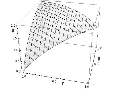
Figure 1: The surface of the von Neumann entropy values of the density matrix (2) depending on the values of $p$ and $r$ parameters.

In the Fig. 1 the von Neumann entropy dependence as a ($p$,$r$)-parameter function is represented: $S(\rho_{CW})=S(p,r)=-Tr(\rho\log\rho)=-\sum_{i}\lambda_{i}\log\lambda_{i}$.

For $p=1$, $r=0$ the von Neumann entropy is zero, and for $p=0$, $r=0$ it reaches its maximal value $S=2$.

The matrix obtained from (4) by partial transpose of states of the first subsystem is the following:

$$\rho^{T_{A}}=\left(\begin{array}[]{cccc}\frac{1}{4}(p+r+1)&0&0&0\\ 0&\frac{1}{4}(1-p-r)&\frac{1}{2}p&0\\ 0&\frac{1}{2}p&\frac{1}{4}(1-p-r)&0\\ 0&0&0&\frac{1}{4}(p+r+1)\\ \end{array}\right),$$ (7)

and after the diagonalization:

$$\rho^{T_{A}}_{diag}=\left(\begin{array}[]{cccc}\frac{1}{4}(p+r+1)&0&0&0\\ 0&\frac{1}{4}(1+p+r)&0&0\\ 0&0&\frac{1}{4}(1+p-r)&0\\ 0&0&0&\frac{1}{4}(1-3p-r)\\ \end{array}\right).$$ (8)

Here eigenvalues $\lambda^{T}_{1}=\frac{1}{4}(1+p+r),\ \ \lambda^{T}_{2}=\frac{1}{4}(1+p+r),\ \ \lambda^{T}_{3}=\frac{1}{4}(1+p-r),\ \ \lambda^{T}_{4}=\frac{1}{4}(1-3p-r)$ are given in a way, that they satisfy the inequality:

$$\lambda^{T}_{1}\geq\lambda^{T}_{2}\geq\lambda^{T}_{3}\geq\lambda^{T}_{4}.$$ (9)

Since $\rho_{CW}$ in (2) is valid only for $0\leq p\leq 1$, $0\leq p+r\leq 1$, then  $\lambda^{T}_{1}$, $\lambda^{T}_{2}$, $\lambda^{T}_{3}$ are nonnegative for any valid values of $p$ and $r$, while $\lambda^{T}_{4}$ is negative for $3p+r>1$. According to the Perec-Horodecki criterion [6, 7] for systems, which consist of two subsystems with the dimensions $m\times n\leq 6$, where $m$ and $n$ are dimensions of first and second subsystem, respectively, the necessary and sufficient condition for the state separability is the condition of non-negativity of all eigenvalues of the density matrix $\rho^{T_{A}}$.

In the case, considered in present paper, the state (2) is separable, and thus unentangled, under the following condition:

$$\left\{\begin{array}[]{ll}3p+r<1,&\hbox{ }\\ 0<p<1.&\hbox{ }\end{array}\right.$$ (10)

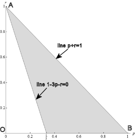
Figure 2: The filled area corresponds to the set of values of $p$ and $r$ parameters, for which the state (2) is inseparable.

In the Fig. 2 the filled area in the $OAB$ triangle corresponds to inseparable (entangled) states. For a fixed value $p<\frac{1}{3}$ a separable state can become inseparable, if one increases the colored noise fraction while reducing the white noise fraction (by increasing the value of the $r$ parameter). For the Werner state ($r=0$) we obtain the well-known result[5]: the state is separable for $p<\frac{1}{3}$.

For $p+r=1$ (white noise absence) one obtains $\lambda_{4}^{T}=-\frac{1}{2}p<0$, which corresponds well to the known statement [8] that under presence of some colored noise fraction and simultaneous absence of white noise the state (2) is remaining entangled (inseparable).

The reduced density matrix of the first and the second subsystem in the state (2) is proportional to the unit matrix: $\rho^{A}=\frac{1}{2}\hat{I}$, $\rho^{B}=\frac{1}{2}\hat{I}$ and independent from $p$ and $r$. Thus, measurement of the polarization state of a single photon in (2) in any orthogonal basis gives the same result.

We now apply the majorization criterion [9] to the state (2).

According to the criterion, if a density matrix $\rho$ is separable, then the following condition is satisfied:

$$\lambda_{\rho}^{\downarrow}\prec\lambda_{\rho_{A}}^{\downarrow}\ \ \ \text{and}\ \ \ \lambda_{\rho}^{\downarrow}\prec\lambda_{\rho_{B}}^{\downarrow},$$ (11)

where $\lambda_{\rho}^{\downarrow}$ denotes the vector, whose components are the eigenvalues of the matrix $\rho$, put in the nonincreasing order, and one can say, that the vector $x^{\downarrow}$ is majorized by the vector $y^{\downarrow}$, if $\sum^{k}_{i=1}x^{\downarrow}_{i}\leq\sum^{k}_{i=1}y^{\downarrow}_{i}$, $k=1,2,3,\ldots,d$, where $d$ is the dimension of the Hilbert space of states and equality is achieved if and only if $k=d$.

In our case

$$x^{\downarrow}=\left(\begin{array}[]{c}\lambda_{1}\\ \lambda_{2}\\ \lambda_{3}\\ \lambda_{4}\\ \end{array}\right),\ \ \ \ \ \ y^{\downarrow}=\left(\begin{array}[]{c}\frac{1}{2}\\ \frac{1}{2}\\ 0\\ 0\\ \end{array}\right),$$

where $\lambda_{1}=\frac{1}{4}(1+3p+r)$,  $\lambda_{2}=\frac{1}{4}(1-p+r)$,  $\lambda_{3}=\frac{1}{4}(1-p-r)$,  $\lambda_{4}=\frac{1}{4}(1-p-r)$.

Then according to the majorization criterion:

$$\left\{\begin{array}[]{ll}\lambda_{1}<\frac{1}{2}&\hbox{ }\\ \lambda_{1}+\lambda_{2}<\frac{1}{2}+\frac{1}{2}&\hbox{ }\\ \lambda_{1}+\lambda_{2}+\lambda_{3}<\frac{1}{2}+\frac{1}{2}+0&\hbox{ }\\ \lambda_{1}+\lambda_{2}+\lambda_{3}+\lambda_{4}=\frac{1}{2}+\frac{1}{2}+0+0&\hbox{ }\end{array}\right.\Rightarrow\left\{\begin{array}[]{ll}3p+r<1&\hbox{ }\\ p+r<1&\hbox{ }\\ p+r<1&\hbox{ }\\ 1=1&\hbox{ }\end{array}\right..$$

The second and the third inequality are always satisfied, if the first inequality is satisfied. Therefore, the state (2) is separable, if the condition $3p+r<1$ is satisfied, which coincides with the condition, obtained from the Perec-Horodecki criterion.

Consider now, under what conditions the state (2) violates the Bell’s inequality in the CHSH form

$$|\beta|\leq 2,$$ (12)

where

$$\ \beta=-\langle A_{0}B_{0}\rangle-\langle A_{0}B_{1}\rangle-\langle A_{1}B_{0}\rangle+\langle A_{1}B_{1}\rangle$$ (13)

is called the Bell operator.

For maximal Bell’s inequality (12) violation analysis, separately in states with white (3) and colored (1) noise, in a paper by Cabello (Adan Cabello at al. [8]) the following onequbit observables were taken:

$$\left\{\begin{array}[]{ll}A_{0}=\sigma_{z},&\hbox{ }\\ A_{1}=\cos(\theta)\sigma_{z}+sin(\theta)\sigma_{x},&\hbox{ }\\ B_{0}=\cos(\phi)\sigma_{z}+sin(\phi)\sigma_{x},&\hbox{ }\\ B_{1}=\cos(\phi-\theta)\sigma_{z}+sin(\phi-\theta)\sigma_{x}.&\hbox{ }\end{array}\right.$$ (14)

The $\theta$ and $\phi$ parameters in (14) determine the orientation of analyzers in experimental devices, $\sigma_{x}$ and $\sigma_{z}$ are the usual Pauli matrices. Computations showed, that for the Werner state (3) the maximal value of $\beta$ as a $p$-parameter function is the following:

$$\beta_{max}(p)=2\sqrt{2}p$$ (15)

and for all values of $p$ the maximal value $\beta$ is obtained by $\theta=\frac{\pi}{2}$, $\phi=\frac{\pi}{4}$.

Thus, Bell’s inequality (12) is violated only for $p>1/\sqrt{2}\approx 0.707$. This implies, that in the case, when the entangled state $|\Phi^{+}\rangle$ is distorted only by white noise, entanglement presence can be detected if noise proportion is less then $\thicksim 29\%$.

In the presence of colored noise (1) the maximal value of $\beta$ for different values of $p$ is achieved at different values of angles $\theta$ and $\phi$. The most interesting fact is that the state (1) violates the CHSH inequality for all values $0<p\leq 1$. Thus, Bell’s inequality violation is extremely robust against colored noise.

In the state (2) the quantity $\beta$, which responds to onequbit observables (14) is a four-parameter function:

$$\begin{split}\beta_{CW}(p,r,\theta,\phi)=cos(\phi)[(2p+r)(sin^{2}(\theta)+cos(\theta))+{}\\ +rcos(\theta)]-sin(\phi)(2p+r)[cos(\theta)-1]sin(\theta).\end{split}$$ (16)

In the colored noise absence $(r=0)$ we have:

$$\beta_{W}(p,\theta,\phi)=2p\{cos(\phi)[sin^{2}(\theta)+cos(\theta)]-sin(\phi)[cos(\theta)-1]sin(\theta)\},$$ (17)

and in the white noise absence $(r=1-p)$:

$$\beta_{C}(p,\theta,\phi)=cos(\phi)[(1+p)sin^{2}(\theta)+2cos(\theta)]-sin(\phi)(1+p)[cos(\theta)-1]sin(\theta).$$ (18)

For fixed values of the $p$ and $r$ parameters the expression (16) is a function of $\theta$ and $\phi$. Solving the extremum problem for the two-variable function, one can find the maximal values $\beta^{max}_{CW}(p,r)$, as well as the angles $\theta$ and $\phi$, that provide the maximal $\beta_{CW}(p,r)$.

In the Fig. 3 the shaded surface graphically displays the $\beta^{max}_{CW}(p,r)$ as a function of two variables $p$ and $r$. For comparison the plane $\beta=2$, which is the boundary value of Bell’s inequality, is also represented in the figure. The surface patch above the plane $\beta=2$ is the CHSH inequality violation area.

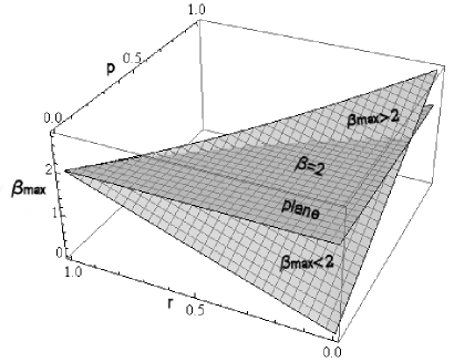
Figure 3: 3D Plot for the maximal Bell operator values, and the $\beta_{CW}=2$ plane, that corresponds to the classical bound.

In the Fig. 4 projections of the traces $\beta=const$ on the $(p,r)$-plane with the surface $\beta^{max}_{CW}(p,r)$ are represented. From the figure one can see that the straight line $p+r=1$ (white noise absence) fully lies in the $\beta^{max}>2$ area, which corresponds to the above conclusion, that Bell’s inequality violation is robust against colored noise. For $r=0$ (colored noise absence) Bell’s inequality is violated only for $p>1/\sqrt{2}$. For any fixed $p$ (pure entangled state weight factor) the value of $\beta^{max}_{CW}$ decreases with the increasing white noise fraction. Thus, as expected, adding some amount of white noise to colored one can reach better agreement of theoretically computed $\beta^{max}$ values with experimental ones. Bell’s inequality violation is unsteady under the increasing of white noise fraction for a fixed total amount (white and colored) of noise.

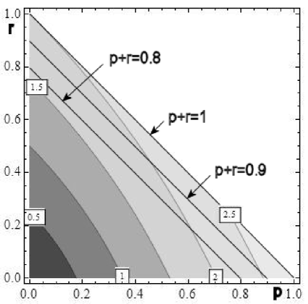
Figure 4: Contour plot for $\beta^{max}(p,r)=const$ - maximal Bell operator values on coordinate plane $(p,r)$.

In the Fig. 5 the $\beta^{max}_{CW}(p,r)$ dependence on $p$ in two boundary cases is given: $r+p=1$ is white noise absence (top curve) and $r=0$ is colored noise absence (bottom dashed straight line). The boundary case dependencies of $\beta^{max}$ on $p$ and $r$ coincide with the ones from the work [4].

Figure 5: Maximal Bell operator values in the case $r=1-p$ is white noise absence(top curve) and $r=0$ is colored noise absence (bottom dashed straight line). Classical bound is $2$. Tsirelson’s bound [10] is $2\sqrt{2}=2.83$.

In the Fig. 6 the values of the angles $\theta$ and $\phi$, that provide maximal values of the Bell operator, are represented. Two solid curves correspond to the case, when in the twophoton polarization state (2) white noise is absent $(p+r=1)$, and two dashed lines correspond to the case, when colored and white noise enter into the expression (2) with the same weight $r=(1-p)/2$. Solid curves coincide with the ones plotted in the work [4]. From the figure one can see that the values of the angles $\theta$ and $\phi$ for a fixed pure entangled state fraction ($p$ is constant) depend on the distribution of weighting coefficients of white and colored noise. Thus, the orientation of the analyzers for obtaining maximal values of $\beta$ depends on the fraction distribution between white and colored noise.

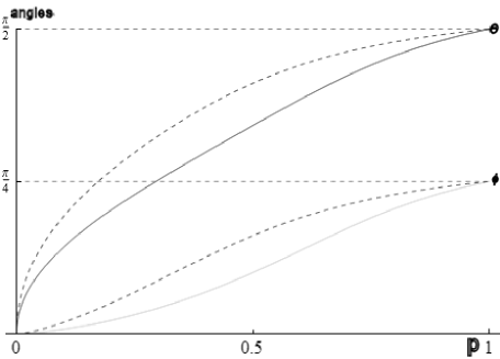
Figure 6: The values of the $\theta$ and $\phi$ parameters that correspond to the maximal Bell operator values (two solid curves concern to the case $r=1-p$ – white noise absence; two dashed curves concern to $r=(1-p)/2$ – equal weight coefficients for white and colored noise).

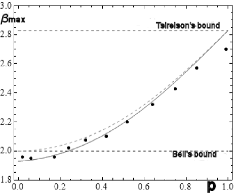
Figure 7: The points represent experimental maximal values of $\beta$ from the work [4]; the dashed curve is the theoretical prediction for the maximal values of $\beta$ in the oneparameter colored noise model [8]; the solid curve shows theoretical calculations in the twoparameter (generalized) noise model with the white noise fraction being $3.5\%$ of the total noise amount in the system.

In the Fig. 7 the points represent the experimental maximal values of $\beta$ from the work [4]; the dashed curve displays theoretical prediction for the maximal values of $\beta$ on the oneparameter colored noise model [8]; the solid curve illustrates theoretical calculations on the twoparameter (generalized) noise model with the white noise fraction being $3.5\%$ of the total noise amount in the system. In the figure we can see that for such a noise proportion experimental data better corresponds to theoretical predictions, i.e. the generalized (twoparameter) noise model is more precise then the oneparameter for the description of realistic states. But in this case too, as one can see in the figure, some experimental points lie above and below the theoretical curve. According to the twoparameter model, this is explained by the fact that by moving from one point to other not only does the total noise amount in the system change, but relative fractions of white and colored noise do too.

Nr.	$p$	$1-p$	white,%	colored,%	$r$
1	0.02	0.98	2	98	0.96
2	0.06	0.97	3	97	0.92
3	0.17	0.83	4	96	0.80
4	0.24	0.76	2	98	0.75
5	0.32	0.68	2	98	0.67
6	0.42	0.58	5	95	0.55
7	0.52	0.48	5	95	0.46
8	0.64	0.36	7	93	0.40
9	0.75	0.25	15	85	0.21
10	0.85	0.15	15	85	0.13

Table of noise proportions in the system.
Correspondence with experimental points in the Fig.7

This kind of interpretation is absolutely logical, because for the each measurement experimental setup is tuned up in a new way (particulary, one has to change the analyzers orientation in space). Remaining in the theoretical model, which is considered in this work, and choosing the corresponding value of the $r$ parameter values for each experimental point (for fixed $p$) one can fully conform theoretical computations with the experimental data. Let us recall, that the preselected values of the parameters $p$ and $r$, according to our model, determine the pure entangled state fraction and relative noise fractions. The percentage of white and colored noise fractions, that give coincidence between theoretical values $\beta_{max}$ and experimental data, are represented in the table. Experimental data were taken from the figure in the work [4].

3 Conclusions

For adequate modeling of the twophoton polarization state, created in the parametric down-conversion process (PDC type II), one should take into account the presence of colored as well as white noise.

The separability condition for the state $\rho_{CW}$, obtained using the Perec-Horodecki criterion is the same as the condition obtained using the majorization criterion. A state $\rho_{CW}$ is separable, when $3p+r<1$.

While Bell’s inequality violation is extremely robust against colored noise (Bell’s inequality is violated for all $0<p\leq 1$), the violation is unsteady under white noise. White noise presence, that is determined by a weighting coefficient of just $0.1$ $(p+r=0.9)$, as one can see in the Fig. 4, leads to Bell’s inequality violation only for $p\gtrsim 0.5$. Simultaneously taking into account both colored and white noise gives possibility to conform theoretical computations with experimental data. Taking $p$ and $r$ as adjustable parameters one can determine colored and white noise fractions by comparison of theoretical calculations with experimental data.

References

- [1] A. Aspect, J. Dalibard, and G. Roger, Phys. Rev. Lett 49, 1804 (1982).
- [2] J. F. Clauser, M. A. Horne, A. Shimony, and R. A. Holt, Phys. Rev. Lett. 23, 880 (1969).
- [3] P. G. Kwait, K. Mattle, H. Weinfurter, A. Zeilinger, A. V. Sergienko, Y. Shih, Phys. Rev. Lett. 75, 4337 (1995).
- [4] F. A. Bovino and G. Castagnoli, A. Cabello, A. Lamas-Linares, Phys. Rev. A 73, 062110 (2006); arXiv: quant-ph/0511265.
- [5] R. F. Werner, Phys. Rev. A 40, 4277 (1989).
- [6] A. Perec, Phys. Rev. Lett. 77, 1413 (1996).
- [7] M. Horodecki, P. Horodecki, and R. Horodecki, Phys. Lett. A 223, 8 (1996).
- [8] A. Cabello and A. Feito, A. Lamas-Linares, Phys. Rev. A 72, 052112 (2005).
- [9] M. Nielsen and J. Kemple, quant-ph/0011117
- [10] B. S. Tsirelson, Lett. Math. Phys. 4, 93 (1980).