Many-body theory of electronic transport in single-molecule heterojunctions

Abstract

A many-body theory of molecular junction transport based on nonequilibrium Green’s functions is developed, which treats coherent quantum effects and Coulomb interactions on an equal footing. The central quantity of the many-body theory is the Coulomb self-energy matrix $\Sigma_{\rm C}$ of the junction. $\Sigma_{\rm C}$ is evaluated exactly in the sequential tunneling limit, and the correction due to finite tunneling width is evaluated self-consistently using a conserving approximation based on diagrammatic perturbation theory on the Keldysh contour. Our approach reproduces the key features of both the Coulomb blockade and coherent transport regimes simultaneously in a single unified transport theory. As a first application of our theory, we have calculated the thermoelectric power and differential conductance spectrum of a benzenedithiol-gold junction using a semi-empirical $\pi$-electron Hamiltonian that accurately describes the full spectrum of electronic excitations of the molecule up to 8–10eV.

I Introduction

Electron transport in single-molecule junctions Nitzan and Ratner (2003, and references therein); Natelson et al. (2006, and references therein); Tao (2006, and references therein) is of fundamental interest as a paradigm for nanosystems far from equilibrium, and as a means to probe important chemicalKuznetso and Ulstrup (1999) and biologicalSchreiber (2005) processes, with myriad potential device applications.Tao (2006, and references therein); Cardamone et al. (2006); Stafford et al. (2007) A general theoretical framework to treat the many-body problem of a single molecule coupled to metallic electrodes does not currently exist. Mean-field approaches based on density-functional theory Todorov et al. (2000); Di Ventra and Lang (2001); Taylor et al. (2001); Heurich et al. (2002); Emberly and Kirczenow (2003); Tomfohr and Sankey (2004); Lindsay and Ratner (2007, and references therein)—the dominant paradigm in quantum chemistry—have serious shortcomings Muralidharan et al. (2006); Ke et al. (2007); Cohen et al. (2008) because they do not account for important interaction effects like Coulomb blockade.

An alternative approach is to solve the few-body molecular Hamiltonian exactly, and treat electron hopping between molecule and electrodes as a perturbation. This approach has been used to describe molecular junction transport in the sequential-tunneling regime,Hettler et al. (2003); Muralidharan et al. (2006); Begemann et al. (2008) but describing coherent quantum transport in this framework remains an open theoretical problem. Higher-order tunneling processes may be treated rigorously in the density-matrix formalism,König et al. (1997); Schoeller and König (2000) but the expansion is typically truncated at fourth order,König et al. (1997); Pedersen and Wacker (2005) the calculation of higher-order terms being prohibitively difficult.

In this article, we develop a many-body theory of molecular junction transport based on nonequilibrium Green’s functionsMeir and Wingreen (1992); Haug and Jauho (1996); Viljas et al. (2005) (NEGF), in order to utilize physically motivated approximations that sum terms of all orders. The junction Green’s functions are calculated exactly in the sequential-tunneling limit, and the corrections to the electron self-energy due to finite tunneling width are included via Dyson-Keldysh equations. The tunneling self-energy is calculated exactly using the equations-of-motions method,Meir et al. (1991); Haug and Jauho (1996) while the correction to the Coulomb self-energy is calculated using diagrammatic perturbation theory. In this way, tunneling processes are included to infinite order, meaning that any approximation utilized is a truncation in the physical processes considered rather than in the order of those processes.

Our approach reproduces the key features of both the Coulomb blockade and coherent transport regimes simultaneously in a single unified transport theory. Nonperturbative effects of intramolecular correlations are included, which are necessary to accurately describe the HOMO-LUMO gap, essential for a quantitative theory of transport.

As a first application of our many-body transport theory, we investigate the benchmark system of benzene(1,4)dithiol (BDT) with gold electrodes. Two key parameters determining the lead-molecule coupling—the tunneling width $\Gamma$ and the chemical potential offset $\Delta\mu$—are fixed by comparison to linear-response measurements of the thermoelectric powerReddy et al. (2007); Baheti et al. (2008) and electrical conductance.Xiao et al. (2004) The nonlinear junction response is then calculated. The differential conductance spectrum of the junction exhibits an irregular “molecular diamond” structure analogous to the regular Coulomb diamondsDe Franceschi et al. (2001) observed in quantum dot transport experiments, as well as clear signatures of coherent quantum transport—such as transmission nodes due to destructive interference—and of resonant tunneling through molecular excited states.

The article is organized as follows: A detailed derivation of the many-body theory of molecular junction transport is presented in Sec. II. Two useful approximate solutions for the nonequilibrium Coulomb self-energy are given in Secs. II.4.1 and II.4.2. The details of the model used to describe a molecular heterojunction consisting of a $\pi$-conjugated molecule covalently bonded to metallic electrodes are presented in Sec. III. The electric and thermoelectric response of a BDT-Au junction are calculated in Sec. IV, and compared to experimental results. A discussion and conclusions are presented in Sec. V.

II Nonequilibrium many-body formalism

II.1 Molecular junction Hamiltonian

The Hamiltonian of a junction consisting of a molecule coupled to several metallic electrodes may be written

$$H_{\rm junction}=H_{\rm mol}+H_{\rm leads}+H_{\rm T}.$$ (1)

The molecular Hamiltonian can be formally divided into one-body and two-body terms $H_{\rm mol}=H^{(1)}_{\rm mol}+H^{(2)}_{\rm mol}$. In general, neglecting spin-orbit coupling, the one-body term can be written

$$H^{(1)}_{\rm mol}=\sum_{n,m,\sigma}\left[H^{(1)}_{\rm mol}\right]_{n\sigma,m\sigma}d_{n\sigma}^{\dagger}d_{m\sigma},$$ (2)

where $d^{\dagger}_{n\sigma}$ creates an electron of spin $\sigma$ on atomic orbital $n$ of the molecule and $[H^{(1)}_{\rm mol}]$ is a hermitian matrix. For simplicity, the atomic basis orbitals are taken to be orthonormal, so that the anticommutator $\{d_{n\sigma}^{\dagger},d_{m\sigma^{\prime}}\}=\delta_{nm}\delta_{\sigma\sigma^{\prime}}$. Extension to non-orthogonal bases is straightforward in principle. For a general spin-rotation invariant two-body (e.g. Coulomb) interaction,

$$H^{(2)}_{\rm mol}=\frac{1}{2}\sum_{n,m}U_{nm}\rho_{n}\rho_{m},$$ (3)

where $\rho_{n}=\sum_{\sigma}d_{n\sigma}^{\dagger}d_{n\sigma}$.

Due to their large density of states (and consequently good screening), the macroscopic metallic electrodes (labeled $\alpha\in[1,\ldots,M]$) may be modeled as non-interacting Fermi gases:

$$H_{\rm leads}=\sum_{\alpha=1}^{M}\sum_{\begin{subarray}{c}k\in\alpha\\ \sigma\end{subarray}}\epsilon_{k\sigma}c_{k\sigma}^{\dagger}c_{k\sigma},$$ (4)

where $c^{\dagger}_{k\sigma}$ creates an electron of energy $\epsilon_{k\sigma}$ in lead $\alpha$. The electrostatic interaction of molecule and electrodes due to the electric dipoles formed at each molecule-electrode interface may be included in $H^{(1)}_{\rm mol}$, as discussed in Sec. III. Tunneling of electrons between the molecule and the electrodes is described by the Hamiltonian

$$H_{\rm T}=\sum_{\alpha=1}^{M}\sum_{k\in\alpha}\sum_{n,\sigma}\left(V_{nk}d_{n\sigma}^{\dagger}c_{k\sigma}+\mathrm{H.c.}\right).$$ (5)

II.2 Non-equilibrium Green’s functions

The electronic system (1) of molecule plus electrodes has an infinite Hilbert space. A formal simplification of the problem is obtained through the use of the Green’s functionsMeir and Wingreen (1992); Haug and Jauho (1996)

$$G_{n\sigma,m\sigma^{\prime}}(t) = -i\theta(t)\langle\{d_{n\sigma}(t),d_{m\sigma^{\prime}}^{\dagger}(0)\}\rangle,$$ (6)

$$G^{<}_{n\sigma,m\sigma^{\prime}}(t) = i\langle d_{m\sigma^{\prime}}^{\dagger}(0)\,d_{n\sigma}(t)\rangle,$$ (7)

known as the retarded and Keldysh “lesser” Green’s functions, respectively. Physical observables in the molecular transport junction can be expressed in terms of $G$ and $G^{<}$. In this section, an exact Dyson equation for $G$ is derived, along with a corresponding Keldysh equation for $G^{<}$.

Setting $\hbar=1$, the retarded Green’s function obeys the equation of motion Haug and Jauho (1996)

$$i\frac{\partial}{\partial t}G_{n\sigma,m\sigma^{\prime}}(t)=\delta(t)\delta_{nm}\delta_{\sigma\sigma^{\prime}}-i\theta(t)\left\langle\left\{\left[d_{n\sigma}(t),H_{\rm junction}\right],d^{\dagger}_{m\sigma^{\prime}}(0)\right\}\right\rangle.$$ (8)

For the purposes of this article, only the spin-diagonal term $G_{n\sigma,m\sigma}$ is needed. Evaluating the commutators $[d_{n\sigma},H_{\rm mol}]$ and $[d_{n\sigma},H_{\rm T}]$, and noting that $[d_{n\sigma},H_{\rm leads}]=0$, Eq. (8) becomes

$$i\frac{\partial}{\partial t}G_{n\sigma,m\sigma}(t)=\delta(t)\delta_{nm}+\sum_{n^{\prime}}\left[H^{(1)}_{\rm mol}\right]_{n\sigma,n^{\prime}\sigma}G_{n^{\prime}\sigma,m\sigma}(t)+\sum_{\alpha}\sum_{k\in\alpha}V_{nk}\,g_{k\sigma,m\sigma}(t)+\sum_{n^{\prime}}U_{nn^{\prime}}G^{(2)}_{n^{\prime},n\sigma m\sigma}(t),$$ (9)

where

$$g_{k\sigma,m\sigma^{\prime}}(t)=-i\theta(t)\left\langle\left\{c_{k\sigma}(t),d^{\dagger}_{m\sigma^{\prime}}(0)\right\}\right\rangle$$ (10)

and

$$G^{(2)}_{n^{\prime},n\sigma m\sigma^{\prime}}(t)=-i\theta(t)\left\langle\left\{\rho_{n^{\prime}}(t)d_{n\sigma}(t),d^{\dagger}_{m\sigma^{\prime}}(0)\right\}\right\rangle.$$ (11)

The equation of motion for $g_{k\sigma,m\sigma}(t)$ is

$$i\frac{\partial}{\partial t}g_{k\sigma,m\sigma}(t)=-i\theta(t)\left\langle\left\{\left[c_{k\sigma}(t),H_{\rm junction}\right],d^{\dagger}_{m\sigma}(0)\right\}\right\rangle.$$ (12)

Evaluating the commutators $[c_{k\sigma},H_{\rm T}]$ and $[c_{k\sigma},H_{\rm leads}]$, and noting that $[c_{k\sigma},H_{\rm mol}]=0$, Eq. (12) becomes

$$i\frac{\partial}{\partial t}g_{k\sigma,m\sigma}(t)=\epsilon_{k\sigma}g_{k\sigma,m\sigma}(t)+\sum_{n^{\prime}}V^{*}_{n^{\prime}k}G_{\rm n^{\prime}\sigma,m\sigma}(t).$$ (13)

Fourier transforming Eqs. (9) and (13) into the energy domain, and eliminating $g_{k\sigma,m\sigma}(E)$, one arrives at the following matrix equation for $G(E)$:

$$\left[{\bf 1}E-H_{\rm mol}^{(1)}-\Sigma_{\rm T}\left(E\right)\right]G(E)={\bf 1}+UG^{(2)}(E),$$ (14)

where the retarded tunneling self-energy matrix is

$$\left[\Sigma_{\rm T}(E)\right]_{n\sigma,m\sigma^{\prime}}=\delta_{\sigma\sigma^{\prime}}\sum_{\alpha}\sum_{k\in\alpha}\frac{V_{nk}V_{mk}^{*}}{E-\epsilon_{k\sigma}+i0^{+}}.$$ (15)

Eq. (14) may be recast in the form of Dyson’s equation

$$G(E)=\left[{\bf 1}E-H_{\rm mol}^{(1)}-\Sigma_{\rm T}(E)-\Sigma_{\rm C}(E)\right]^{-1}$$ (16)

via the ansatz $UG^{(2)}(E)\equiv\Sigma_{\rm C}(E)G(E)$, which defines Mahan (1990) the retarded Coulomb self-energy matrix $\Sigma_{\rm C}(E)$, the central quantity of the many-body theory, which must be determined via an appropriate approximation, as discussed below.

For nonequilibrium problems, the Keldysh “lesser” self-energy and Green’s function are also needed. $G^{<}$ is determined by the Keldysh equation Haug and Jauho (1996)

$$G^{<}(E)=G(E)\Sigma^{<}(E)G^{\dagger}(E),$$ (17)

where $\Sigma^{<}(E)=\Sigma_{\rm T}^{<}(E)+\Sigma_{\rm C}^{<}(E)$, and $G^{\dagger}(E)$ is the Fourier transform of the advanced Green’s function. The “lesser” tunneling self-energy is

$$\left[\Sigma_{\rm T}^{<}(E)\right]_{n\sigma,m\sigma^{\prime}}=i\sum_{\alpha}f_{\alpha}(E)\left[\Gamma^{\alpha}(E)\right]_{n\sigma,m\sigma^{\prime}}^{*},$$ (18)

where $f_{\alpha}(E)=\{1+\exp[(E-\mu_{\alpha})/k_{B}T_{\alpha}]\}^{-1}$ is the Fermi-Dirac distribution for lead $\alpha$, and

$$\left[\Gamma^{\alpha}(E)\right]_{n\sigma,m\sigma^{\prime}}=2\pi\delta_{\sigma\sigma^{\prime}}\sum_{k\in\alpha}V_{nk}^{*}V_{mk}\,\delta(E-\epsilon_{k\sigma})$$ (19)

is the tunneling-width matrix for lead $\alpha$.

Once the Green’s functions are known, the relevant physical observables can be calculated. For example, the current flowing into lead $\alpha$ is given by Meir and Wingreen (1992)

$$I_{\alpha}=\frac{ie}{h}\int dE\;{\rm Tr}\left\{\Gamma^{\alpha}(E)\left(G^{<}(E)+f_{\alpha}(E)\left[G(E)-G^{\dagger}(E)\right]\right)\right\}.$$ (20)

II.3 Sequential tunneling limit

In the limit of infinitessimal lead-molecule coupling $\Sigma_{\rm T}/k_{B}T\rightarrow 0$, coherent superpositions of different energy eigenstates of the molecule can be neglected, and the junction Green’s function becomes

$$\lim_{\Sigma_{\rm T}\rightarrow 0}\left[G(E)\right]_{n\sigma,m\sigma}\equiv\left[G_{\rm mol}(E)\right]_{n\sigma,m\sigma}=\sum_{\nu,\nu^{\prime}}\left[{\cal P}(\nu)+{\cal P}(\nu^{\prime})\right]\frac{\langle\nu|d_{n\sigma}|\nu^{\prime}\rangle\langle\nu^{\prime}|d_{m\sigma}^{\dagger}|\nu\rangle}{E-E_{\nu^{\prime}}+E_{\nu}+i0^{+}},$$ (21)

where $|\nu\rangle$ and $|\nu^{\prime}\rangle$ are many-body eigenstates of the isolated molecule satisfying $H_{\rm mol}|\nu\rangle=E_{\nu}|\nu\rangle$, etc. The nonequilibrium probabilities ${\cal P}(\nu)$ can be determined by solving a system of semiclassical rate equations for sequential tunneling.Beenakker (1991); Hettler et al. (2003); Muralidharan et al. (2006); Begemann et al. (2008) For steady-state transport, they satisfy the principle of detailed balance (see Fig. 1):

$${\cal P}(\nu)\sum_{\alpha}\tilde{\Gamma}^{\nu\nu^{\prime}}_{\alpha}\!f_{\alpha}\left(E_{\nu^{\prime}}-E_{\nu}\right)={\cal P}(\nu^{\prime})\sum_{\alpha}\tilde{\Gamma}^{\nu\nu^{\prime}}_{\alpha}\!\left[1-f_{\alpha}\left(E_{\nu^{\prime}}-E_{\nu}\right)\right].$$ (22)

Here the rate constants are given by Fermi’s Golden rule as

$$\tilde{\Gamma}^{\nu\nu^{\prime}}_{\alpha}={\rm Tr}\left\{\Gamma^{\alpha}(E_{\nu^{\prime}}-E_{\nu})C^{\nu\nu^{\prime}}\right\},$$ (23)

where $\Gamma^{\alpha}(E)$ is given by Eq. (19) and

$$[C^{\nu\nu^{\prime}}]_{n\sigma,m\sigma^{\prime}}=\langle\nu|d_{n\sigma}|\nu^{\prime}\rangle\langle\nu^{\prime}|d_{m\sigma^{\prime}}^{\dagger}|\nu\rangle$$ (24)

are many-body matrix elements.Kinaret et al. (1992); Stafford (1996); Stafford et al. (1998) From the normalization of the many-body wavefunctions, the total resonance width $\tilde{\Gamma}^{\nu\nu^{\prime}}=\sum_{\alpha}\tilde{\Gamma}^{\nu\nu^{\prime}}_{\alpha}$ scales as $\mbox{}\sim\sum_{\alpha}\mbox{Tr}\{\Gamma^{\alpha}\}/N$, where $N$ is the number of atomic orbitals in the molecule. For strongly-correlated systems, there is an additional exponential suppression of Eq. (24) as $N\rightarrow\infty$ due to the orthogonality catastrophe.Stafford et al. (1998); Anderson (1967)

Linear response transport is determined by the equilibrium Green’s functions. In equilibrium, the solution of the set of Eqs. (22) reduces to

$${\cal P}(\nu)=e^{-\beta(E_{\nu}-\mu N_{\nu})}/{\cal Z},$$ (25)

where ${\cal Z}$ is the grand partition function of the molecule at inverse temperature $\beta$ and chemical potential $\mu$.

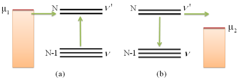
Figure 1: A schematic representation of detailed balance. The left-hand and right-hand sides of Eq. (22) are represented in (a) and (b), respectively.

Eq. (21) implicitly defines the Coulomb self-energy matrix $\Sigma_{\rm C}^{(0)}$ in the sequential tunneling limit via

$$G_{\rm mol}(E)=\left[{\bf 1}E-H_{\rm mol}^{(1)}-\Sigma_{\rm C}^{(0)}(E)\right]^{-1}.$$ (26)

$\Sigma_{\rm C}^{(0)}$ is the high-temperature limit of the Coulomb self-energy (i.e., the limit $k_{B}T/\mbox{Tr}\{\Gamma^{\alpha}\}\gg 1$), and describes intramolecular correlations and charge quantization effects (Coulomb blockade away from resonance). The nonperturbative treatment of intramolecular correlations provided by exact diagonalization of $H_{\rm mol}$ in Eq. (21) allows for an accurate description of the HOMO-LUMO gap, which is essential for a quantitative theory of transport.

II.4 Correction to the Coulomb self-energy

In general, the Coulomb self-energy matrix $\Sigma_{\rm C}=\Sigma_{\rm C}^{(0)}+\Delta\Sigma_{\rm C}$, where $\Delta\Sigma_{\rm C}$ describes the change of the Coulomb self-energy due to lead-molecule coherence emerging at temperatures $k_{B}T\lesssim\mbox{Tr}\{\Gamma^{\alpha}\}$. Using this decomposition of the Coulomb self-energy, Dyson’s equation (16) can be rewritten in the following useful form:

$$G^{-1}(E)=G_{\rm mol}^{-1}(E)-\Sigma_{\rm T}-\Delta\Sigma_{\rm C},$$ (27)

where the self-energy terms $\Sigma_{\rm T}+\Delta\Sigma_{\rm C}$ describe the effects of finite tunneling width. $\Sigma_{\rm T}$ is given by Eq. (15). Here we point out that $\Delta\Sigma_{\rm C}$—unlike $\Sigma_{\rm C}^{(0)}$—can be evaluated perturbatively using diagrammatic techniques on the Keldysh time-contour (cf. Fig. 2). Such a perturbative approach is valid, in principle, at temperatures/bias voltages satisfying $\max\{T,eV/k_{B}\}>T_{K}$, where $T_{K}$ is the Kondo temperaturePustilnik and Glazman (2004, and references therein)—or when there is no unpaired electron on the molecule (such as within the HOMO-LUMO gap of conjugated organic molecules).

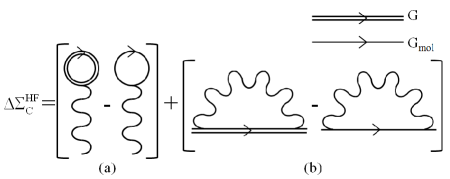
Figure 2: The correction to the Coulomb self-energy $\Delta\Sigma_{\rm C}$ is given in the self-consistent Hartree-Fock approximation by the sum of (a) the Hartree (direct) term and (b) the Fock (exchange) term. The wavy line represents the Coulomb interaction, which has the form $U_{nm}\delta(\tau-\tau^{\prime})$ on the Keldysh time contour.

$\Sigma_{\rm T}+\Delta\Sigma_{\rm C}$ may be thought of as the response of the junction to turning on the tunneling coupling $\Gamma^{\alpha}$. A subtlety in the perturbative evaluation of $\Delta\Sigma_{\rm C}$ is that the diagrams determining the Coulomb self-energy are typically formulatedMahan (1990) in terms of the Green’s functions of the noninteracting system, $G^{(0)}(E)=({\bf 1}E-H_{\rm mol}^{(1)}-\Sigma_{\rm T})^{-1}$ and $G^{(0)}_{\rm mol}(E)=({\bf 1}E-H_{\rm mol}^{(1)}+i0^{+})^{-1}$, while the response of the junction is determined by the full Green’s function $G(E)$ [cf. Eq. (20)]. Evaluating the diagrams in Fig. 2 using $G^{(0)}(E)$ and $G^{(0)}_{\rm mol}(E)$ would yield a correction to the Coulomb self-energy with a pole structure unrelated to that of $\Sigma_{\rm C}^{(0)}$, so that adding the two together would not yield a physically meaningful result. Our strategy is thus to calculate $\Delta\Sigma_{\rm C}$ by reformulating the terms in the perturbative expansion in terms of the full Green’s function $G(E)$ via appropriate resummations. This procedure is in general nontrivial, but the result for the Hartree-Fock correction is given in Sec. II.4.2 below, based on physical arguments. Higher-order self-energy diagrams can be included in a similar fashion. Electron-phonon couplingMitra et al. (2004); Galperin et al. (2004); Paulsson et al. (2005); Viljas et al. (2005); de la Vega et al. (2006); Solomon et al. (2006) can also be included in the many-electron theory via the self-energy terms $\Sigma_{\rm e-ph}+\Delta\Sigma_{\rm C}^{\rm e-ph}$, where $\Sigma_{\rm e-ph}$ is given by the usual self-energy diagrams,Galperin et al. (2004); Paulsson et al. (2005); Viljas et al. (2005); de la Vega et al. (2006); Solomon et al. (2006) and $\Delta\Sigma_{\rm C}^{\rm e-ph}$ is the corresponding correction to the Coulomb self-energy.

II.4.1 Elastic cotunneling approximation: $\Sigma=\Sigma_{\rm T}+\Sigma_{\rm C}^{(0)}$

Far from transmission resonances and for $T\gg T_{K}$, $\Delta\Sigma_{\rm C}$ can be neglected. This is the limit of elastic cotunneling.Averin and Nazarov (1990); Groshev et al. (1991) The Green’s functions are given by Eqs. (16) and (17), with $\Sigma_{\rm C}=\Sigma_{\rm C}^{(0)}$. Note that $[\Sigma_{\rm C}^{(0)}]^{<}$ does not make a finite contribution to Eq. (17) when $\Sigma_{\rm T}$ is finite. The full NEGF current expression (20) then reduces to the multi-terminal Büttiker formula Büttiker (1986)

$$I_{\alpha}=\frac{2e}{h}\sum_{\beta=1}^{M}\int_{-\infty}^{\infty}dE\;T_{\beta\alpha}(E)\left[f_{\beta}(E)-f_{\alpha}(E)\right],$$ (28)

where the transmission function is given byDatta (1995)

$$T_{\beta\alpha}(E)={\rm Tr}\left\{\Gamma^{\alpha}(E)G(E)\Gamma^{\beta}(E)G^{\dagger}(E)\right\}.$$ (29)

The elastic cotunneling approximation is a conserving approximation—current is conserved [cf. Eq. (28)] and the spectral function obeys the usual sum-rule.

II.4.2 Self-consistent Hartree-Fock correction: $\Sigma_{\rm C}=\Sigma_{\rm C}^{(0)}+\Delta\Sigma_{\rm C}^{\rm HF}$

In the Hartree-Fock (HF) approximation, the retarded Coulomb self-energy matrix is given by

$$\left[\Sigma_{\rm C}^{\rm HF}\right]_{n\sigma,m\sigma^{\prime}}=\delta_{\sigma\sigma^{\prime}}\left[\delta_{nm}\sum_{n^{\prime}}U_{nn^{\prime}}\langle\rho_{n^{\prime}}\rangle-U_{nm}\langle d^{\dagger}_{m\sigma}d_{n\sigma}\rangle\right],$$ (30)

and $\left[\Sigma_{\rm C}^{\rm HF}\right]^{<}=0$. In general,

$$\langle d_{n\sigma}^{\dagger}d_{m\sigma^{\prime}}\rangle=-\frac{i}{2\pi}\int_{-\infty}^{\infty}dE\,[G^{<}(E)]_{m\sigma^{\prime},n\sigma}$$ (31)

and

$$\lim_{\Sigma_{\rm T}\rightarrow 0}\langle d_{n\sigma}^{\dagger}d_{m\sigma^{\prime}}\rangle=\sum_{\nu}{\cal P}(\nu)\langle\nu|d_{n\sigma}^{\dagger}d_{m\sigma^{\prime}}|\nu\rangle.$$ (32)

The Hartree-Fock correction is then $\Delta\Sigma_{\rm C}^{\rm HF}\equiv\Sigma_{\rm C}^{\rm HF}-\Sigma_{\rm C}^{\rm HF}|_{\Sigma_{\rm T}\rightarrow 0}$. The Feynman diagrams representing this correction are shown in Fig. 2. A self-consistent solution of Eqs. (17), (27), and (30)–(32) yields a conserving approximation in which the junction current is again given by Eq. (28).

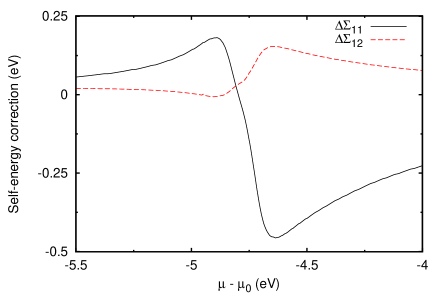
Figure 3: Self-consistent Hartree-Fock correction to the Coulomb self-energy matrix of a diatomic molecule versus lead chemical potential, shown in the vicinity of the HOMO resonance. Here $\mu_{0}=\left(\varepsilon_{\rm HOMO}+\varepsilon_{\rm LUMO}\right)/2$ is the chemical potential of the isolated molecule, $T=300\mbox{K}$, and $\Gamma_{1}=\Gamma_{2}=0.2\mbox{eV}$ (see Sec. III).

The use of the interacting Green’s functions $G$ and $G_{\rm mol}$ in the evaluation of the Hartree self-energy is clearly justified on physical grounds, since this yields the classical electrostatic potential due to the actual nonequilibrium charge distribution on the molecule. The direct (Hartree) and exchange (Fock) contributions to $\Delta\Sigma_{\rm C}$ must be treated on an equal footing in order to cancel the unphysical self-interaction, justifying the use of the same interacting Green’s functions in the evaluation of the exchange self-energy. The diagrams of Fig. 2 would be quite complex if expressed in terms of noninteracting Green’s functions, because both $G$ and $G_{\rm mol}$ involve $\Sigma_{\rm C}^{(0)}$, which includes all possible combinations of Coulomb lines and intramolecular propagators.

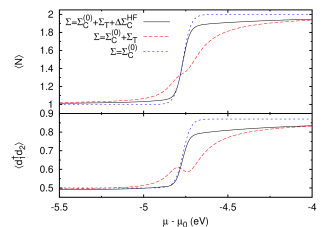
Figure 4: Equilibrium correlation functions near the HOMO resonance for a diatomic molecule (same parameters as in Fig. 3). Top: Total molecular charge $\langle N\rangle$ in three different approximations: $\Sigma=\Sigma_{\rm C}^{(0)}$ (isolated molecule in the grand canonical ensemble); $\Sigma=\Sigma_{\rm C}^{(0)}+\Sigma_{\rm T}$ (elastic cotunneling approximation); and $\Sigma=\Sigma_{\rm C}^{(0)}+\Sigma_{\rm T}+\Delta\Sigma_{\rm C}^{\rm HF}$ (self-consistent HF correction). The charging step is broadened in the elastic cotunneling approximation, compared to that of the isolated molecule, and acquires a ‘knee’ near resonance. In the self-consistent HF approximation, the charge imbalance $\Delta N=\langle N\rangle-\langle N\rangle|_{\Sigma_{\rm T}\rightarrow 0}$ is strongly screened near resonance, leading to a charging step as steep as that of the isolated molecule, but asymptotically approaches the elastic cotunneling result away from resonance. Bottom: The correlation function $\langle d^{\dagger}_{1\sigma}d_{2\sigma}\rangle$ in the same three approximations.

The self-consistent Hartree-Fock correction for a diatomic molecule is shown in Fig. 3. The parameters were chosen so that the resonance width $\mbox{}\sim\sum_{\alpha}\mbox{Tr}\{\Gamma^{\alpha}\}/N=0.2\mbox{eV}$, where $N$ is the number of atomic orbitals in the molecule. The elements of the matrix $\Delta\Sigma_{\rm C}^{\rm HF}$ are largest near a transmission resonance, but vanish on resonance. This behavior can be understood by considering the molecular correlation functions shown in Fig. 4. Inclusion of the tunneling self-energy without the corresponding correction to the Coulomb self-energy leads to a charge imbalance on the molecule near resonance. This in turn leads to a Hartree correction which tends to counteract the charge imbalance. A corresponding behavior is found for the exchange correction and off-diagonal correlation function. A non-self-consistent calculation would yield a much larger correction $\Delta\Sigma_{\rm C}^{\rm HF}$, indicating the important role of screening. It should be pointed out that a treatment of screening in linear response is not adequate near resonance.

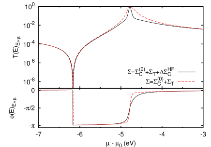
Figure 5: Transmission probability and phase calculated with and without the self-consistent HF correction. Note that the transmission peaks and nodes are not shifted by $\Delta\Sigma_{\rm C}^{\rm HF}$, but the width of the transmission resonance is reduced asymmetrically.

As shown in Fig. 5, the transmission peaks and nodes are not shifted by the self-consistent HF correction, and the transmission phase is not changed significantly. Transport properties [cf. Eqs. (28) and (29)] are therefore qualitatively better described in the elastic cotunneling approximation than are the correlation functions, and the approximation is quantitatively accurate in the cotunneling regime $|\mu-\mu_{\rm res}|>\Gamma$, $\max\{T,eV/k_{B}\}>T_{K}$.

The tendency toward charge quantization near resonance is significantly increased by the self-consistent HF correction, as shown in Fig. 4. The steepness of the self-consistent charging step is limited only by thermal broadening. This result is consistent with previous theoretical studiesGolubev and Zaikin (1994); Matveev (1995); Göppert and Grabert (2001, and references therein) of Coulomb blockade in metal islands and quantum dots, but inconsistent with the behavior of the Anderson model,Pustilnik and Glazman (2004, and references therein) where singular spin fluctuations modify this generic behavior.

III Molecular Heterojunction Model

Heterojunctions formed from $\pi$-conjugated molecules are of particular interest, both because of their relevance for nanotechnologyTao (2006, and references therein); Cardamone et al. (2006) and their extensive experimental characterization.Nitzan and Ratner (2003, and references therein); Natelson et al. (2006, and references therein); Tao (2006, and references therein) A semi-empirical $\pi$-electron Hamiltonian Chandross et al. (1997); Castleton and Barford (2002); Cardamone et al. (2006) can be used to model the electronic degrees of freedom most relevant for transport:

$$H_{\rm mol}=\sum_{n,\sigma}\varepsilon_{n}d_{n\sigma}^{\dagger}d_{n\sigma}-\sum_{n,m,\sigma}\left(t_{nm}d_{n\sigma}^{\dagger}d_{m\sigma}+\mathrm{H.c.}\right)\mbox{ }+\sum_{n,m}\frac{U_{nm}}{2}Q_{n}Q_{m},\,\,\,\,$$ (33)

where $d^{\dagger}_{n\sigma}$ creates an electron of spin $\sigma$ in the $\pi$-orbital of the $n$th carbon atom, $\varepsilon_{n}$ is the atomic orbital energy, and $t_{nm}$ is the hopping matrix element between orbitals $n$ and $m$. In the $\pi$-electron theory, the effect of different side-groups is included through shifts of the orbital energies $\varepsilon_{n}$. The effect of substituents (e.g., thiol groups) used to bond the leads to the molecule can be includedTian et al. (1998); Nitzan (2001) in the tunneling matrix elements $V_{nk}$ [cf. Eq. (5)].

The effective charge operator for orbital $n$ isStafford et al. (1998); Cardamone et al. (2006)

$$Q_{n}=\sum_{\sigma}d_{n\sigma}^{\dagger}d_{n\sigma}-\sum_{\alpha}C_{n\alpha}\mathcal{V}_{\alpha}/e-1,$$ (34)

where $C_{n\alpha}$ is the capacitive coupling between orbital $n$ and lead $\alpha$, $e$ is the electron charge, and $\mathcal{V}_{\alpha}$ is the voltage on lead $\alpha$. The lead-molecule capacitances are elements of a full capacitance matrix $C$, which also includes the intra-molecular capacitances, determined by the relation $C_{nm}=e^{2}[U^{-1}]_{nm}$. The values $C_{n\alpha}$ are determined by the zero-sum rules required for gauge invarianceLandau et al. (1984)

$$\sum_{m}C_{nm}+\sum_{\alpha=1}^{M}C_{n\alpha}=0,$$ (35)

and by the geometry of the junction (e.g. $C_{n\alpha}$ inversely proportional to lead-orbital distance).

The effective interaction energies for $\pi$-conjugated systems can be writtenChandross et al. (1997); Castleton and Barford (2002)

$$U_{nm}=\delta_{nm}U_{0}+\left(1-\delta_{nm}\right)\frac{U_{0}}{\epsilon\sqrt{1+\alpha(R_{nm}/\mbox{\AA})^{2}}},$$ (36)

where $U_{0}$ is the on-site Coulomb repulsion, $\alpha=\left(U_{0}/14.397\mbox{eV}\right)^{2}$, and $R_{nm}$ is the distance between orbitals $n$ and $m$. The phenomenological dielectric constant $\epsilon$ accounts for screening due to both the $\sigma$-electrons and any environmental considerations, such as non-evaporated solvent.Castleton and Barford (2002) With an appropriate choice of the parameters $t_{nm}$, $U_{0}$, and $\epsilon$, the complete spectrum of electronic excitations up to 8–10eV of the molecules benzene, biphenyl, and trans-stilbene in the gas phase can be reproduced with high accuracyCastleton and Barford (2002) by exact diagonalization of Eq. (33). An accurate description of excited states is essential to model transport far from equilibrium. Larger conjugated organic molecules can also be modeled Chandross et al. (1997); Chakrabarti and Mazumdar (1999) via Eqs. (33) and (36).

$\sigma$-orbitals can also be included in Eq. (33) as additional energy bands, and the resulting multi-band extended Hubbard model can be treated using the same NEGF formalism sketched above. Tunneling through the $\sigma$-orbitals may be important in small molecules,Ke et al. (2008); Solomon et al. (2008a) especially in cases where quantum interference leads to a transmission node in the $\pi$-electron system.

The biggest uncertainty in modelling single-molecule heterojunctions is the lead-molecule coupling.Ke et al. (2005) For this reason, we take the two most uncertain quantitites characterizing lead-molecule coupling—the tunneling width $\Gamma$ and the chemical potential offset $\Delta\mu$ of isolated molecule and metal electrodes—as phenomenological parameters to be determined by fitting to experiment. In the broad-band limitJauho et al. (1994) for the metallic electrodes, and assuming each electrode is covalently bonded to a single carbon atom of the molecule, the tunneling-width matrix reduces to a single constant: $\Gamma_{nm}^{\alpha}(E)=\Gamma_{\alpha}\delta_{na}\delta_{ma}$, where $a$ is the orbital connected to electrode $\alpha$. Typical estimates Mujica et al. (1994); Tian et al. (1998); Nitzan (2001) indicate $\Gamma\lesssim 1\mbox{eV}$ for organic molecules coupled to gold contacts via thiol groups.

IV Benzene(1,4)dithiol junction

As a first application of our many-body theory of molecular junction transport, we consider the benchmark system of benzene(1,4)dithiol (BDT) with two gold leads.Reed et al. (1997); Reichert et al. (2003); Xiao et al. (2004); Dadosh et al. (2005); Kriplani et al. (2006); Toher and Sanvito (2007); Reddy et al. (2007); Baheti et al. (2008) The Hamiltonian parameters for benzene areCastleton and Barford (2002) $U_{0}=8.9\mbox{eV}$, $\epsilon=1.28$, $t_{nm}=2.68\mbox{eV}$ for $n$ and $m$ nearest neighbors, and $t_{nm}=0$ otherwise. We consider a symmetric junction (symmetric capacitive couplings and $\Gamma_{1}=\Gamma_{2}\equiv\Gamma$) at room temperature (T=300K).

IV.1 Linear electric and thermoelectric junction response

Thermoelectric effects Paulsson and Datta (2003); Reddy et al. (2007); Baheti et al. (2008) provide important insight into the transport mechanism in single-molecule junctions, but are particularly sensitive to correlations,Chaikin and Beni (1976); Stafford (1993) calling into question the applicability of single-particle or mean-field theory. We can now investigate thermoelectric effects in molecular heterojunctions for the first time using many-body theory. The thermopower $S$ of a molecular junction is obtained by measuring the voltage $\Delta{\cal V}\equiv-S\Delta T$ created across an open junction in response to a temperature differential $\Delta T$. In general, $S$ can be calculated by taking the appropriate linear-response limit of Eq. (20), which includes both elastic and inelastic processes. However, for purely elastic transport [cf. Secs. II.4.1 and II.4.2], Eq. (28) can be used to derive the well-known resultSivan and Imry (1986); van Houten et al. (1992)

$$S(\mu,T)=-\frac{1}{\mbox{eT}}\frac{\int_{-\infty}^{\infty}T_{12}(E)\left(-\frac{\partial f}{\partial E}\right)\left(E-\mu\right)dE}{\int_{-\infty}^{\infty}T_{12}(E)\left(-\frac{\partial f}{\partial E}\right)dE}.$$ (37)

Thermopower measurementsBaheti et al. (2008); Reddy et al. (2007) provide a means to determinePaulsson and Datta (2003) the lead-molecule chemical potential mismatch $\Delta\mu=\mu_{\rm Au}-\mu_{0}$, where $\mu_{0}=\left(\varepsilon_{\rm HOMO}+\varepsilon_{\rm LUMO}\right)/2$ and $\varepsilon_{\rm HOMO}$ ($\varepsilon_{\rm LUMO}$) is the HOMO (LUMO) energy level. Figure 6 shows the thermopower of a BDT junction as a function of $\Delta\mu$, calculated from Eqs. (29) and (37) in the elastic cotunneling approximation. As pointed out by Paulsson and Datta,Paulsson and Datta (2003) $S$ is nearly independent of $\Gamma$ away from the transmission resonances, allowing $\Delta\mu$ to be determined directly by comparison to experiment. The thermopower of a BDT-Au junction was recently measured by Baheti et al.,Baheti et al. (2008) who obtained the result $S=(7.0\pm 0.2)\mu\mbox{V}/\mbox{K}$. Equating this experimental value with the calculated thermopower shown in Fig. 6, we find that $-3.25{\rm eV}\leq\mu_{\rm Au}-\mu_{0}\leq-3.15{\rm eV}$ over a broad range of $\Gamma$ values. The Fermi level of gold thus lies about $1.8\mbox{eV}$ above the HOMO resonance, validating the notion that transport in these junctions is hole-dominated. Nonetheless, $\mu_{\rm Au}-\varepsilon_{\rm HOMO}$ is sufficiently large that the elastic cotunneling approximation is well justified.

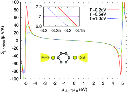
Figure 6: Thermoelectric power of a BDT-Au junction at $T=300$K as a function of the lead-molecule chemical potential mismatch for three different tunneling widths. Comparison to the experimental valueBaheti et al. (2008) $7.0\pm 0.2\mu\mbox{V}/\mbox{K}$ fixes $\mu_{\rm Au}=\mu_{0}-(3.22\pm 0.04)\mbox{eV}$ (see inset showing closeup of experimentally relevant parameter range).

The only other free parameter in the molecular junction model is the tunneling width $\Gamma$, which can be found by matching the linear-response conductance to experiment. Although there is a large range of experimental values,Lindsay and Ratner (2007, and references therein) the most reproducible and lowest resistance contacts were obtained by Xiao, Xu and Tao,Xiao et al. (2004) who report a single-molecule conductance value of 0.011G₀. This fixes $\Gamma=(0.63\pm 0.02)\mbox{eV}$ with $\mu_{\rm Au}-\mu_{0}=-3.22\pm 0.04\mbox{eV}$. This value of $\Gamma$ is within the range predicted by other groups for similar molecules.Mujica et al. (1994); Tian et al. (1998); Nitzan (2001); Ke et al. (2005) With the final parameter in the model fixed, we can now use our many-body transport theory to predict the linear and nonlinear response of this molecular junction.

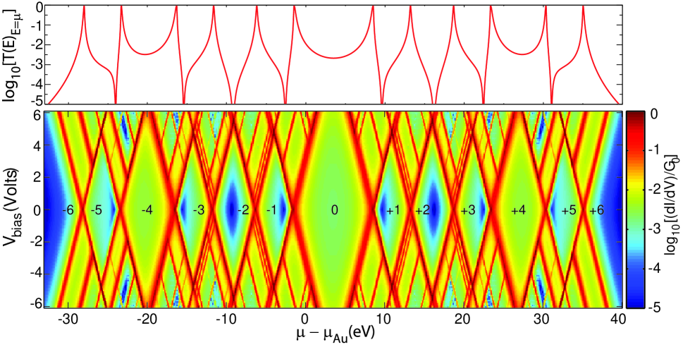
Figure 7: Linear-response conductance versus chemical potential (top panel) and differential conductance versus chemical potential and bias voltage (bottom panel) for a benzene(1,4)dithiol–Au junction. The calculation was carried out within the elastic cotunneling approximation using Eq. (28), with $\Gamma_{1}=\Gamma_{2}=0.6\mbox{eV}$ and $T=300\mbox{K}$. Here $G_{0}=2e^{2}/h$ is the conductance quantum. Note the asymmetric Fano-like lineshapes and the transmission nodes (arising from destructive interference) in the top panel. The numbers within the central diamonds of the bottom panel indicate the quantized charge on the molecule (relative to neutral benzene). The full spectrum is shown for completeness.

The transmission probability $T(E)|_{E=\mu}$ of the BDT junction is shown as a function of $\mu-\mu_{\rm Au}$ in the upper panel of Fig. 7. This is the linear-response conductance in units of the conductance quantum $G_{0}=2e^{2}/h$. The chemical potential $\mu$ is related to the gate voltage $V_{g}$ in a three-terminal junction via the gate capacitance $C_{g}$. The transmission spectrum shown in Fig. 7 exhibits several striking features: a large but irregular peak spacing with an increased HOMO-LUMO gap, non-symmetric, Fano-like resonance lineshapes, and transmission nodes due to destructive interference in the coherent quantum transport.

IV.2 Non-linear junction transport

We next calculate the differential conductance $\partial I/\partial V_{\rm bias}$ of the BDT-Au junction as a function of $\mu$ and $V_{\rm bias}$ (see Fig. 7, lower panel). The current was calculated in the elastic cotunneling approximation using Eqs. (28) and (29). This approximation accurately describes nonresonant transport, including the transmission nodes, as well as the positions and heights of the transmission resonances, as discussed in Sec. II.4.2. The differential conductance spectrum of the junction exhibits clear signatures of excited-state transport Weis et al. (1993); De Franceschi et al. (2001) and an irregular “molecular diamond” structure analogous to the regular Coulomb diamonds observed in quantum dot transport experiments.De Franceschi et al. (2001) The charge on the molecule is quantized within the central diamonds of Fig. 7, an important interaction effect inaccessible to so-called ab initio mean-field calculations. In Fig. 7, the full spectrum is shown for completeness, although the junction may not be stable over the entire range of bias and gate voltages shown.

Apart from the central HOMO-LUMO gap, the widths of the diamonds in Fig. 7 can be roughly explained via a capacitive model in which the molecule is characterized by a single capacitance $C_{\rm mol}=e^{2}/\left\langle U_{nm}\right\rangle$, where $\left\langle U_{nm}\right\rangle=5.11\mbox{eV}$ is the average over all molecular sites. The HOMO-LUMO gap of $\sim$10eV is significantly larger than this estimate of the charging energy, an indication of the significant deviations of our theory from a simple constant interaction model.

Charge quantization, also known as Coulomb blockade, has been observed in several different types of molecular heterojunctions,Park et al. (2000); Liang et al. (2002); Kubatkin et al. (2003); Poot et al. (2006); Danilov et al. (2008) but has not yet been observed in BDT junctions due to the difficulty of gating such small molecules.Li et al. (2006) The unambiguous observation of Coulomb blockade in junctions involving larger molecules (with smaller charging energies) indicates that such interaction effects, lying outside the scope of mean-field approaches, are undoubtedly even more pronounced in small molecules like BDT. Important aspects of this phenomenon remain to be understood in larger molecules, such as the anomalously low reported values of the charging energy.Park et al. (2000); Liang et al. (2002); Kubatkin et al. (2003); Poot et al. (2006); Danilov et al. (2008)

A zero-bias cross section of the bottom panel of Fig. 7 reproduces the transmission spectrum shown in the top panel of the same figure. Increasing the bias voltage, we find that the resonances split into negatively sloped particle-like ($|e|dV/d\mu=-\left(C_{1}+C_{2}+C_{g}\right)/C_{1}$) lines and positively sloped hole-like ($|e|dV/d\mu=+\left(C_{1}+C_{2}+C_{g}\right)/C_{2}$) lines, where $C_{1}$ and $C_{2}$ are the mean lead-molecule capacitances, defined by $C_{\alpha}=\langle C_{n\alpha}\rangle$, $\alpha=1,2$. In the symmetric coupling case ($C_{1}=C_{2}$ with $C_{g}/C_{1}\ll 1$) the lines therefore have slopes of -2 and +2 for particle-like and hole-like lines, respectively. Within the V-shaped outline traced by the particle-like and hole-like lines, we find signatures of resonant tunneling through electronic excited states in the many narrow, nearly parallel resonance lines. While transport through electronic excited states has not yet been unambiguously identified in single-molecule heterojunctions, it has been observed in quantum dotsWeis et al. (1993); De Franceschi et al. (2001) and carbon nanotubes.Sapmaz et al. (2006)

An accurate description of the HOMO-LUMO gap is essential for a quantitative theory of transport in molecular heterojunctions. The central HOMO-LUMO gap shown in Fig. 7 is significantly larger than that predictedNitzan and Ratner (2003, and references therein) by density functional theory—which neglects charge-quantization effects—but is consistent with previous many-body calculations in the sequential tunneling regime.Hettler et al. (2003); Muralidharan et al. (2006); Begemann et al. (2008) It should be emphasized that the transport gap $\Delta\mu_{\rm tr}$ in a molecular junction exceeds the optical gap $\hbar\omega_{\rm min}$ of an isolated molecule. Roughly speaking, $\Delta\mu_{\rm tr}\simeq\hbar\omega_{\rm min}+e^{2}/C_{\rm mol}+E_{x}$, where $e^{2}/C_{\rm mol}$ is the charging energy (see discussion above) and $-E_{x}$ is the exciton binding energy. Excitonic states of the BDT-Au junction can be identified in the differential conductance spectrum of Fig. 7 as the lowest-energy (i.e., smallest bias) excitations outside the central diamond of the HOMO-LUMO gap, from which it is apparent that $\Delta\mu_{\rm tr}\approx 2\hbar\omega_{\rm min}$ for a BDT-Au junction.

V Conclusions

In conclusion, we have developed a many-body theory of electron transport in single-molecule heterojunctions that treats coherent quantum effects and Coulomb interactions on an equal footing. As a first application of our theory, we have investigated the thermoelectric power and differential conductance of a prototypical single-molecule junction, benzenedithiol with gold electrodes.

Our results reproduce the key features of both the coherent and Coulomb blockade transport regimes: Quantum interference effects, such as the transmission nodes predicted within mean-field theory,Cardamone et al. (2006); Solomon et al. (2008a, b) are confirmed, while the differential conductance spectrum exhibits characteristic charge quantization “diamonds”Park et al. (2000); Liang et al. (2002); Kubatkin et al. (2003); Poot et al. (2006); Danilov et al. (2008)—an effect outside the scope of mean-field approaches based on density-functional theory. The HOMO-LUMO transport gap obtained is consistent with previous many-body treatments in the sequential tunneling limit.Hettler et al. (2003); Muralidharan et al. (2006); Begemann et al. (2008)

The central object of the many-body theory is the Coulomb self-energy $\Sigma_{\rm C}$ of the junction, which may be expressed as $\Sigma_{\rm C}=\Sigma_{\rm C}^{(0)}+\Delta\Sigma_{\rm C}$, where $\Sigma_{\rm C}^{(0)}$ is the result in the sequential tunneling limit, and $\Delta\Sigma_{\rm C}$ is the correction due to a finite tunneling width $\Gamma$. In this article, we have evaluated $\Sigma_{\rm C}^{(0)}$ exactly, thereby including intramolecular correlations at a nonperturbative level, while the direct and exchange contributions to $\Delta\Sigma_{\rm C}$ were evaluated self-consistently using a conserving approximation based on diagrammatic perturbation theory on the Keldysh contour. An important feature of our theory is that this approximation for $\Delta\Sigma_{\rm C}$ can be systematically improved by including additional processes diagrammatically. In this way, important effects such as dynamical screening, spin-flip scattering,Pustilnik and Glazman (2004, and references therein) and electron-phonon couplingMitra et al. (2004); Galperin et al. (2004); Paulsson et al. (2005); Viljas et al. (2005); de la Vega et al. (2006); Solomon et al. (2006) can be included as natural extensions of the theory.

Our general theory of molecular junction transport should be contrasted to results for transport in the Anderson model.Pustilnik and Glazman (2004, and references therein); Galperin et al. (2007) The Anderson model provides important insight into nonperturbative interaction effects in quantum transport through nanostructures; however, the internal structure of the molecule is neglected. Moreover, since it is limited to a single spin-degenerate level, it can only describe a single Coulomb diamond with an odd number of electrons on the molecule, and is therefore not applicable to transport within the HOMO-LUMO gap of conjugated organic molecules, where the number of electrons is even (more precisely, the HOMO-LUMO gap is taken to be infinite in the Anderson model).

Recently, a NEGF approach for molecular junction transport was introduced Galperin et al. (2008) using Green’s functions that are matrices in a basis of many-body molecular eigenstate outer products $|\nu\rangle\langle\nu^{\prime}|$; it is unclear what relation this approach has to the approach proposed herein involving single-particle Green’s functions, which are matrices in the atomic orbital basis.