Coulomb blockade double-dot Aharonov-Bohm interferometer: giant fluctuations

Abstract

Electron transport through two parallel quantum dots is a kind of solid-state realization of double-path interference. We demonstrate that the inter-dot Coulomb correlation and quantum coherence would result in strong current fluctuations with a divergent Fano factor at zero frequency. We also provide physical interpretation for this surprising result, which displays its generic feature and allows us to recover this phenomenon in more complicated systems.

Introduction.— As an analogue of Young’s double-slit interference Feynman et al. (1970), electron interfering through mesoscopic systems, e.g., a ring-like Aharonov-Bohm (AB) interferometer with a quantum dot in one of the interfering paths, is of interest for many fundamental reasons Hackenbroich (2001). The AB oscillation of conductance has been observed in both closed Yacoby et al. (1995) and open geometry Buk98 , together with elegant theoretical analysis Aha02 . Recently, further study was carried out for the closed-loop setup, with particular focus on the multiple-reflection induced inefficient “which path” information by a nearby charge detector Kang08 .

Going beyond the mere quantum interference, incorporation of Coulomb correlation between the two paths should be of great interest. This can be realized by transport through parallel double dots (DD) in Coulomb blockade regime. For such DD setup, existing studies include the cotunneling interference Loss and Sukhorukov (2000); Los-01 ; König and Gefen (2001); Sig06 , and two-loops (two fluxes) interference with the two dots as an artificial molecule Hol0102 ; Jia02 . Remarkably, super-Poisson noise and giant Fano Factor were predicted in this system, as generated by the Coulomb correlations Los-01 ; Wang et al. (2007); Dong08 .

It was very recently found Li0803 that the Coulomb blockade in parallel dots pierced by magnetic flux $\Phi$ completely blocks the resonant current for any value of $\Phi$ except for integer multiples of the flux quantum $\Phi_{0}$. It was shown there that this effects in a quantum analogue of self-trapping phenomenon in non-linear systems. In the present paper we concentrate on Coulomb blockade effects in parallel dots, where dephasing and lossy channels are included. In particular we concentrate on the shot-noise spectrum. We demonstrate that in the absence of dephasing and lossy channels this quantity diverges at zero frequency. The most important result of our analysis is an explanation of this phenomenon using symmetry arguments. This explanation displays a new way for a simple treatment of complicated Coulomb blockade effects in the presence of quantum interference.

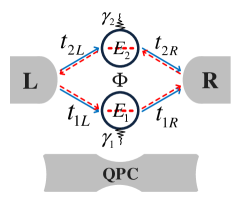
Figure 1: (Color online) Schematic setup of a double-dot Aharonov-Bohm interferometer. To address dephasing and electron-loss effects, a nearby quantum-point-contact (QPC) detector and lossy channels (with strength $\gamma_{1(2)}$) are introduced.

Model.— Consider double dots (DD) connected in parallel to two leads. For simplicity we assume that in each of the dots there is only one level, $E_{1}$ and $E_{2}$, involved in the transport. Also, we neglect the spin degrees of freedom. In case of strong Coulomb blockade, the effect of spin can be easily restored by doubling the tunneling rates of each QD with the left lead. The system is described by the following Hamiltonian,

$$H=H_{0}+H_{T}+\sum_{\mu=1,2}E_{\mu}d_{\mu}^{\dagger}d_{\mu}+Ud_{1}^{\dagger}d_{1}d_{2}^{\dagger}d_{2}\,.$$ (1)

Here the first term, $H_{0}=\sum_{k}[E_{kL}a_{kL}^{\dagger}a_{kL}+E_{kR}a_{kR}^{\dagger}a_{kR}]$, describes the leads and $H_{T}$ describes their coupling to the dots,

$$H_{T}=\sum_{\mu,k}\Big{(}t_{\mu L}d_{\mu}^{\dagger}a_{kL}+t_{\mu R}a_{kR}^{\dagger}d_{\mu}\Big{)}+{\rm H.c.}\,,$$ (2)

where $\mu=1,2$ and $a_{kL}^{\dagger}$ and $a_{kR}^{\dagger}$ are the creation operators for the electrons in the leads while $d_{1,2}^{\dagger}$ are the creation operators for the DD. The last term in Eq. (1) describes the interdot repulsion. We assume that there is no tunnel coupling between the dots and that the couplings of the dots to the leads, $t_{\mu L(R)}$, are independent of energy. In the absence of a magnetic field one can always choose the gauge in such a way that all couplings are real. In the presence of a magnetic flux $\Phi$, however, the tunneling amplitudes between the dots and the leads are in general complex. We write $t_{\mu L(R)}={\bar{t}}_{\mu L(R)}e^{i\phi_{\mu L(R)}}$, where $\bar{t}_{\mu L(R)}$ is the coupling without the magnetic field. The phases are constrained to satisfy $\phi_{1L}+\phi_{1R}-\phi_{2L}-\phi_{2R}=\phi$, where $\phi\equiv 2\pi\Phi/\Phi_{0}$.

To account for dephasing effect, we introduce a “which path” measurement by a nearby point contact (PC) detector Buk98 , with a model description as in Ref. Wang et al., 2007. To make contact with conventional double-slit interferometer, we also introduce electron lossy channels. Slightly differing from Ref. Aha02, , instead of the semi-infinite tight binding chain introduced there, we model the lossy channels by attaching each dot with an electronic side reservoir, which is particularly suited in the master equation approach. The side-reservoir model was originally proposed by Büttiker in dealing with phase-breaking effect But8688 , i.e., electron would lose phase information after entering the reservoir first, then returning back from it. But here, we assume that the reservoir’s Fermi level is much lower than the dot energy. As a result, electron only enters the reservoir unidirectionally, never coming back.

Formalism.— The transport properties of the above described system, both current and fluctuations, can be conveniently studied by the number-resolved master equation Gur96 ; Li et al. (2005a); Luo et al. (2007). The central quantity of this approach is the number-conditioned state, $\rho^{(n)}(t)$ of the double dots, where $n$ is the electron number passed through the junction between the DD and an assigned lead where number counting is done. Very usefully, $\rho^{(n)}(t)$ is related to the electron-number distribution function, in terms of $P(n,t)={\rm Tr}[\rho^{(n)}(t)]$, where the trace is over the DD states. From $P(n,t)$ the current and its fluctuations can be readily analyzed. For current, it simply reads $I(t)=ed\langle n(t)\rangle/dt$, where $\langle n(t)\rangle=\sum_{n}nP(n,t)$. For current fluctuations, we employ the MacDonald’s formula, $S(\omega)=2\omega\int_{0}^{\infty}dt\sin\omega t\frac{d}{dt}[\langle n^{2}(t)\rangle-(\bar{I}t)^{2}]$, to calculate the noise spectrum. Here, $\langle n^{2}(t)\rangle=\sum_{n}n^{2}P(n,t)$, and $\bar{I}$ is the stationary current. In practice, instead of directly solving $P(n,t)$, the reduced quantity $\langle n^{2}(t)\rangle$ can be obtained more easily by constructing its equation of motion, based on the “$n$”-resolved master equation Li et al. (2005a); Luo et al. (2007).

Under inter-dot Coulomb blockade, i.e., the DD can be simultaneously occupied at most by one electron, the Hilbert space of the DD state is reduced to $|0\rangle\equiv|00\rangle$, $|1\rangle\equiv|10\rangle$, and $|2\rangle\equiv|01\rangle$, where $|10\rangle$ means the upper dot occupied and the lower dot unoccupied, and other states have similar interpretations. Following Ref. Luo et al., 2007, the “$n$”-resolved master equation in this basis can be straightforwardly carried out as

$$\dot{\rho}^{(n)}_{00}=-2\Gamma_{L}\rho_{00}^{(n)}+\left(\gamma+\Gamma_{R}\right)\rho_{11}^{(n-1)}+\left(\gamma+\Gamma_{R}\right)\rho_{22}^{(n-1)}+e^{i\left(\phi_{\text{R1}}-\phi_{\text{R2}}\right)}\Gamma_{R}\rho_{12}^{(n-1)}+e^{i\left(\phi_{\text{R2}}-\phi_{\text{R1}}\right)}\Gamma_{R}\rho_{21}^{(n-1)}$$ (3a)

$$\dot{\rho}_{11}^{(n)}=\Gamma_{L}\rho_{00}^{(n)}-\left(\gamma+\Gamma_{R}\right)\rho_{11}^{(n)}-\frac{1}{2}e^{i\left(\phi_{\text{R1}}-\phi_{\text{R2}}\right)}\Gamma_{R}\rho_{12}^{(n)}-\frac{1}{2}e^{i\left(\phi_{\text{R2}}-\phi_{\text{R1}}\right)}\Gamma_{R}\rho_{21}^{(n)}$$ (3b)

$$\dot{\rho}_{22}^{(n)}=\Gamma_{L}\rho_{00}^{(n)}-\left(\gamma+\Gamma_{R}\right)\rho_{22}^{(n)}-\frac{1}{2}e^{i\left(\phi_{\text{R1}}-\phi_{\text{R2}}\right)}\Gamma_{R}\rho_{12}^{(n)}-\frac{1}{2}e^{i\left(\phi_{\text{R2}}-\phi_{\text{R1}}\right)}\Gamma_{R}\rho_{21}^{(n)}$$ (3c)

$$\dot{\rho}_{12}^{(n)}=e^{i\left(\phi_{\text{L1}}-\phi_{\text{L2}}\right)}\Gamma_{L}\rho_{00}^{(n)}-\frac{1}{2}e^{i\left(\phi_{\text{R2}}-\phi_{\text{R1}}\right)}\Gamma_{R}\rho_{11}^{(n)}-\frac{1}{2}e^{i\left(\phi_{\text{R2}}-\phi_{\text{R1}}\right)}\Gamma_{R}\rho_{22}^{(n)}-\frac{1}{2}\left(\gamma_{d}+2\gamma+2i\Delta+2\Gamma_{R}\right)\rho_{12}^{(n)}$$ (3d)

$$\dot{\rho}_{21}^{(n)}=e^{i\left(\phi_{\text{L2}}-\phi_{\text{L1}}\right)}\Gamma_{L}\rho_{00}^{(n)}-\frac{1}{2}e^{i\left(\phi_{\text{R1}}-\phi_{\text{R2}}\right)}\Gamma_{R}\rho_{11}^{(n)}-\frac{1}{2}e^{i\left(\phi_{\text{R1}}-\phi_{\text{R2}}\right)}\Gamma_{R}\rho_{22}^{(n)}-\frac{1}{2}\left(\gamma_{d}+2\gamma-2i\Delta+2\Gamma_{R}\right)\rho_{21}^{(n)}$$ (3e)

In the above equations, $\Delta=E_{1}-E_{2}$ is the offset of the dot levels. $\Gamma_{L(R)}=2\pi D_{L(R)}|t_{L(R)}|^{2}$, and $\gamma_{1(2)}=2\pi D_{1(2)}|t_{1(2)}|^{2}$, are the respective rates for the couplings to the left and right leads, as well as to the side reservoirs. $D_{L(R)}$ and $D_{1(2)}$ are the density of states of the leads and reservoirs, while $t_{L(R)}$ and $t_{1(2)}$ are the respective tunneling amplitudes. Note that in actual calculation presented in this paper we replaced $\Gamma_{L}$ with $2\Gamma_{L}$ (c.f. Gur96 ; Luo et al. (2007)). In this work we assume that $\gamma_{1}=\gamma_{2}=\gamma$. Finally, $\gamma_{d}$ characterizes dephasing between the two dots, resulting for instance from the “which path” measurement by the point contact.

Note that the master equations (3a)-(3e) include the off-diagonal density-matrix elements, so that they explicitly display their quantum mechanical nature. However these equations can be derived from the many-body Scrödinger equation only in the infinite bias limit in the presence of Coulomb blockade Gur96 ; Li et al. (2005a); Luo et al. (2007).

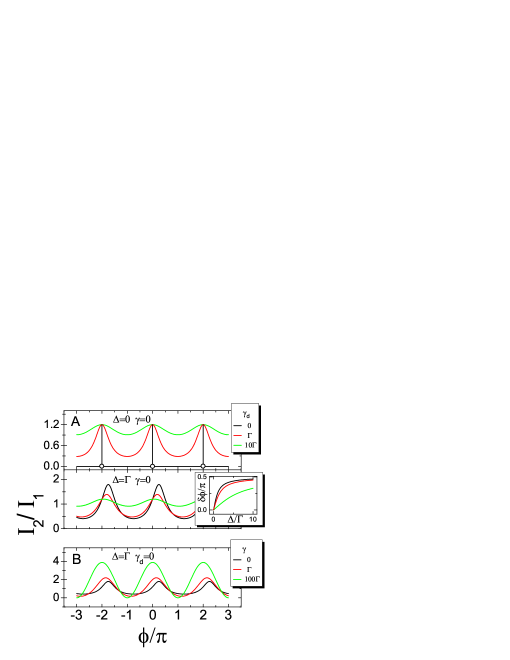
Figure 2: (Color online) (A) Current switch and dephasing effect under closed geometry ($\gamma=0$) for aligned DD levels ($\Delta=0$). (B) Phase shift for $\Delta\neq 0$ and electron loss effect. With increasing the lossy strength $\gamma$, the conventional double-slit interference pattern is recovered.

Current.— First, we consider the case without electron loss, i.e., $\gamma=0$. Simple expression for the steady-state current is extractable:

$$I=\left\{\frac{2(\gamma_{\rm d}\!+\!2\Gamma_{\rm R})(1\!-\!\cos\phi)-4\Delta\sin\phi}{\gamma_{\rm d}(\gamma_{\rm d}+2\Gamma_{\rm R})+4\Delta^{2}}+\frac{1}{I_{0}}\right\}^{-1},$$ (4)

where $I_{0}=4\Gamma_{\rm L}\Gamma_{\rm R}/(4\Gamma_{\rm L}+\Gamma_{\rm R})$, is the current in the absence of magnetic flux. However, in the following we will use the current of transport through a Coulomb-blockade single dot, $I_{1}=2\Gamma_{\rm L}\Gamma_{\rm R}/(2\Gamma_{\rm L}+\Gamma_{\rm R})$, to scale the double-dot current, in order to highlight the interference features.

For the limiting case $\gamma_{d}$=0, i.e., no dephasing between the two dots, from Eq. (4) we have $I=I_{0}\Delta^{2}/\{\Delta^{2}+I_{0}[\Gamma_{R}(1-\cos\phi)-\Delta\sin\phi]\}$. Then a novel switching effect follows this result: as $\Delta\rightarrow 0$, $I=I_{0}$ for $\phi=2\pi n$, while $I=0$ for any deviation of $\phi$ from these values. This remarkable behavior can be explained by defining new basis states of the DD, $d^{\dagger}_{\mu}|0\rangle\to\tilde{d}^{\dagger}_{\mu}|0\rangle$, chosen such that $\tilde{d}^{\dagger}_{2}|0\rangle$ is not coupled to the right reservoir, i.e., $t_{2R}\to\tilde{t}_{2R}=0$, then the current would flow only through the state $\tilde{d}_{1}^{\dagger}|0\rangle$. This can be realized by the unitary transformation Li0803

$$\left(\begin{array}[]{c}\widetilde{d}_{1}\\ \widetilde{d}_{2}\end{array}\right)={1\over{\cal N}}\left(\begin{array}[]{cc}t_{1R}&t_{2R}\\ -t^{*}_{2R}&t^{*}_{1R}\end{array}\right)\left(\begin{array}[]{c}d_{1}\\ d_{2}\end{array}\right),$$ (11)

with ${\cal N}=(\bar{t}_{1R}^{2}+\bar{t}_{2R}^{2})^{1/2}$, which indeed results in $\widetilde{t}_{2R}=0$. Also, the coupling of $\widetilde{d}^{\dagger}_{2}|0\rangle$ to the left lead reads

$$\widetilde{t}_{2L}(\phi)=-e^{i(\phi_{2L}-\phi_{1R})}(\bar{t}_{1L}\bar{t}_{2R}\,e^{i\phi}-\bar{t}_{2L}\bar{t}_{1R})/{\cal N}.$$ (12)

It follows from this expression that $\widetilde{t}_{2L}=0$ for $\phi=2n\pi$ provided that $\bar{t}_{1L}/\bar{t}_{2L}=\bar{t}_{1R}/\bar{t}_{2R}$, or for $\phi=(2n+1)\pi$ if $\bar{t}_{1L}/\bar{t}_{2L}=-\bar{t}_{1R}/\bar{t}_{2R}$. Obviously, for noninteracting DD, $\widetilde{d}^{\dagger}_{2}|0\rangle$ has no contribution to current, while $\widetilde{d}^{\dagger}_{1}|0\rangle$ carries a magnetic-flux modulated current. In the case of inter-dot Coulomb blockade, however, whether the coupling of $\widetilde{d}^{\dagger}_{2}|0\rangle$ to the left lead is zero becomes of crucial importance. If $\widetilde{t}_{2L}\neq 0$, then the state $\widetilde{d}_{1}^{\dagger}|0\rangle$, carrying the current, will be blocked by the inter-dot Coulomb repulsion. As a result, the total current vanishes. However, if the state $\widetilde{d}_{2}^{\dagger}|0\rangle$ is decoupled from both leads, it remains unoccupied, so that the current can flow through the state $\widetilde{d}_{1}^{\dagger}|0\rangle$. As shown above, this takes place precisely for $\bar{t}_{1L}/\bar{t}_{2L}=\pm\,\bar{t}_{1R}/\bar{t}_{2R}$. If this condition is not fulfilled, the current is always zero, even for $\phi=2\pi n$.

As we demonstrated above, the switching effect becomes very transparent in the particular basis of the DD states. Still, it is very surprising how such a basis emerges dynamically? Indeed, an electron from the left lead can enter the DD system in any of SU(2) equivalent superpositions of its states. Therefore there exists a probability for each electron to enter the DD in the superposition that eliminates one of the links with the right lead. When it happens, the electron would be trapped in this state. Even if the probability of this event for one electron is very small, the total number of electrons passing through the DD goes to infinity for $t\rightarrow\infty$. Therefore the trapping event is always realized for large enough time. In the presence of Coulomb blockade this would lead to the switching effect, as explained above.

In the presence of dephasing, which is modelled by a which-path detection in this work, the switching effect discussed above will be smeared out, as shown in Fig. 2(A). In appearance, the resultant interference pattern resembles the usual one of the double-slit interferometer. However, both qualitatively and quantitatively, there exists remarkable differences, e.g., the unchanged current at $\phi=2\pi n$, which is also the fully dephased current.

As the DD levels deviate from alignment, i.e., $\Delta\neq 0$, the current switching phenomena will also disappear, as shown in Fig. 2(B). Similar to dephasing, from Eq. (4), we see that the current at $\phi=2\pi n$ is unaffected by $\Delta$, too. However, for $\Delta\neq 0$, this is not the maximal current. Accordingly, a phase shift of the interference pattern is implied. In more generic sense, this is nothing but the breaking of phase locking But86 , for two-terminal transport which can appear only under finite bias voltage and typically in the presence of electron-electron interactions König and Gefen (2001).

In Fig. 2(B) we display also the effect of electron loss. That is, we introduce lossy channels to make the interferometer more and more open. As a result, we see that all the above distinguished features disappear and the conventional double-slit interference pattern is restored by increasing the lossy strength $\gamma$. The basic reason is that, as the dots become increasingly open, the side reservoirs would reduce the occupation probability on the dots, thus make the Coulomb correlation and back-reflection less important.

Current Fluctuations.— Current fluctuations are usually characterized by the zero-frequency shot noise, which can be calculated by the particle-number-resolved master equation approach, using the MacDonald’s formula as sketched in the formalism. Strikingly, for the present Coulomb blockade DD interferometer, we find that the zero-frequency shot noise can be highly super-Poissonian, and can even become divergent as $\Delta\rightarrow 0$. In the following we first demonstrate this novel result, then show more other features of the noise.

For coherent DD interferometer, analytical result of the frequency-dependent noise can be obtained using the MacDonald’s formula:

$$S(\omega)=\frac{8\Gamma_{L}\Gamma_{R}[2\Gamma_{L}\Gamma_{R}\Delta^{2}-\Delta^{4}+3\Delta^{2}\omega^{2}-2\omega^{2}(\Gamma^{2}_{R}+\omega^{2})]\bar{I}}{[(2\Gamma_{L}+\Gamma_{R})\Delta^{2}-(2\Gamma_{L}+3\Gamma_{R})\omega^{2}]^{2}+\omega^{2}(2\Gamma_{L}\Gamma_{R}+2\Gamma^{2}_{R}+\Delta^{2}-\omega^{2})^{2}}+2\bar{I}~{}.$$ (13)

Here we have assumed $\phi=2\pi n$. At zero frequency limit, the Fano factor reads

$$F\equiv\frac{S(0)}{2\bar{I}}=\frac{8\Gamma^{2}_{L}\Gamma^{2}_{R}+(4\Gamma^{2}_{L}+\Gamma^{2}_{R})\Delta^{2}}{(2\Gamma_{L}+\Gamma_{R})^{2}\Delta^{2}}.$$ (14)

Strikingly, as $\Delta\rightarrow 0$, it becomes divergent! Note that this divergence is not caused by the average current $\bar{I}$, but the zero-frequency noise itself. Very interestingly, from Eq. (13), we find that the limiting order of $\Delta\rightarrow 0$ and $\omega\rightarrow 0$, would lead to different results. That is, if we first make $\Delta\rightarrow 0$, then $\omega\rightarrow 0$, the result reads

$$F=\frac{\Gamma^{2}_{L}+\Gamma^{2}_{R}}{(\Gamma_{L}+\Gamma_{R})^{2}},$$ (15)

which is finite and coincides with the Fano factor of single-level transport Luo et al. (2007). The limiting order leading to Eq. (15) implies that we are considering the noise for aligned DD levels. In this case, as constructed above, see Eq. (11) and Fig. 3(a), the two transformed dot-states are decoupled to each other, and one of them also decoupled to both leads if $\phi=2\pi n$. As a result, equivalently, the transport is through a single channel, leading to the Fano factor Eq. (15).

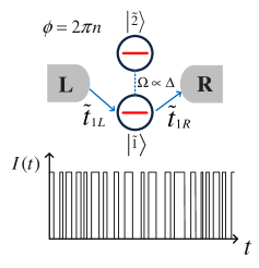
Figure 3: (Color online) Schematic interpretation for the noise divergence. Upper panel: Effective coupling of the DD to the leads and between the dots, in the representation of transformed DD states, i.e., $|\tilde{1}\rangle\equiv\tilde{d}^{\dagger}_{1}|0\rangle$ and $|\tilde{2}\rangle\equiv\tilde{d}^{\dagger}_{2}|0\rangle$. Lower panel: Coarse-grained temporal current, with a telegraphic noise nature which causes divergence of the zero-frequency noise when $\Delta\rightarrow 0$ .

However, for $\Delta\rightarrow 0$ but $\neq 0$, the situation is subtly different. In this case, the two transformed states are weakly coupled, with a strength $\propto\Delta$. Thus, the transporting electron on state $\tilde{d}_{1}^{\dagger}|0\rangle$ can occasionally tunnel to $\tilde{d}_{2}^{\dagger}|0\rangle$, which is disconnected to both leads, and its occupation will block the current until the electron tunnels back to $\tilde{d}_{1}^{\dagger}|0\rangle$ and arrives at the right lead. Typically, this strong bunching behavior, induced by the interplay of Coulomb interaction and quantum interference, is well characterized by a profound super-Poissonian statistics. In Fig. 3(b), the coarse-grained temporal current with a telegraphic noise nature is plotted schematically. We see that, as $\Delta\rightarrow 0$, the current switching would become extremely slow, leading to very long time ($\sim 1/\Delta$) correlation between the transport electrons. It is right this long-time-scale fluctuation, or equivalently, the low frequency component filtered out from the current, which causes divergence of the shot noise as $\Delta\rightarrow 0$. This is similar, in certain sense, to the well known $1/f$ noise, which goes to divergence as $f\rightarrow 0$.

It is quite interesting that a similar divergence of the noise-spectrum at zero frequency has been found for rather broad conditions (but only for inelastic cotunneling regime) in the framework of classical master equations. The latter neglects the off-diagonal elements of the density matrix and assumes weak enough tunneling Los-01 . In contrast, our quantum rate equations approach goes beyond these assumptions. On the other hand it shows that the switching effect and divergency of the noise-spectrum can take place only at the large bias voltage Li0803 . Indeed, by applying the unitary transformation (11), one can always decouple one of the states from the right reservoir. However, one still needs the total occupation of this state at $t\to\infty$. Otherwise the Coulomb blockade is not complete and so the switching effect. This condition can be realized only in the large bias limit, where the energy levels of the dots are far from the corresponding Fermi energy.

Magnetic-Flux Dependence.— The previous study was restricted to zero magnetic flux so that only the state $\tilde{d}_{1}^{\dagger}|0\rangle$ is connected to the leads. Now we proceed to nonzero magnetic flux and $\Delta\neq 0$. In this case, $\tilde{\Gamma}_{1L}(\phi)$ and $\tilde{\Gamma}_{2L}(\phi)$ are nonzero in general. By tuning the flux from $\phi=0$ to $\pi$, the effective coupling $\tilde{\Gamma}_{2L}$ is switched on, while $\tilde{\Gamma}_{1L}$ switched off. As a result, the strong current fluctuation at $\phi=0$ is considerably suppressed owing to this transition to transport through $\tilde{d}_{1}^{\dagger}|0\rangle$ and $\tilde{d}_{2}^{\dagger}|0\rangle$ in series. In between $\phi=0$ and $\pi$, however, we find a local minimum for the Fano factor, with a common value given by Eq. (15), being independent of $\Delta$. Its location in $\phi$, however, depends on $\Delta$. This is because, for different $\Delta$, one can always find a proper $\phi$, such that $\tilde{d}_{1}^{\dagger}|0\rangle$ couples to the left lead, both directly and indirectly through $\tilde{d}_{2}^{\dagger}|0\rangle$, with an effective coupling strength $\Gamma_{L}$. Remind also that, the coupling of $\tilde{d}_{1}^{\dagger}|0\rangle$ to the right lead is $\sim\Gamma_{R}$. Accordingly, the Fano factor of Eq. (15) is reached.

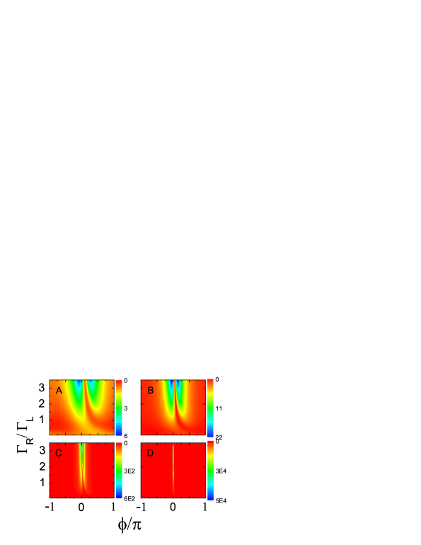
Figure 4: (Color online) Contour plot of the Fano factor versus the (scaled) magnetic flux $\phi$ and tunnel-coupling asymmetry $\Gamma_{R}/\Gamma_{L}$, for different DD level detuning: $\Delta=\Gamma$ (A), $0.5\Gamma$ (B), $0.1\Gamma$ (C), and $0.01\Gamma$ (D).

In Fig. 4, we display the Fano factor versus the (scaled) magnetic flux (phase difference $\phi$) and the tunnel-coupling asymmetry $\Gamma_{R}/\Gamma_{L}$. Besides the $\phi$-dependence, we see that, with the increase of $\Gamma_{R}/\Gamma_{L}$, the Fano factor is considerably enhanced and becomes highly super-Poissonian. Interpretation for this dependence is referred to Ref. Wang et al., 2007, where the concept of effective fast-to-slow channels was proposed.

Finally, not shown in Fig. 4 includes the effects of dephasing and electron loss. It is clear that, for dephased (original) dots, we can no longer construct the superposition states $\tilde{d}_{1}^{\dagger}|0\rangle$ and $\tilde{d}_{2}^{\dagger}|0\rangle$. Then, the fast-to-slow channel induced bunching behavior is not anticipated, and the Fano factor is reduced to the Poissonian value. For lossy effect, we conclude that, with increasing the lossy strength ($\gamma$), shorter duration time on dots will weaken the role of Coulomb interaction and multiple reflections, making the noise characteristics Poissonian, like that from usual random emission.

Note Added.— After the submission of present work to the arXiv:0812.0846-eprint, a very recent paper by Urban and König was caused into our attention Urb08 , where the enhancement of shot noise and even divergence were found in the absence of inter-dot but in the presence of intra-dot Coulomb blockade. In that case, the electron spin plays an essential role. In our DD Coulomb blockade regime, however, the electron spin is irrelevant to the super-Poisson noise and its divergence.

Acknowledgments.— This work was supported by the National Natural Science Foundation of China under grants No. 60425412 and No. 90503013. X.Q.L. acknowledges the Albert Einstein Minerva Center for Theoretical Physics for partially supporting his visit to the Weizmann Institute of Science. S.G is grateful to the Max Planck Institute for the Physics of Complex Systems, Dresden, Germany for kind hospitality.

References

- Feynman et al. (1970) R. P. Feynman, R. B. Leighton, and M. Sands, The Feynman Lectures on Physics, Vol. III, Chap. 1. (Addison-Wesley, Reading, 1970).
- Hackenbroich (2001) G. Hackenbroich, Phys. Rep. 343, 463 (2001).
- Yacoby et al. (1995) A. Yacoby, M. Heiblum, D. Mahalu, and H. Shtrikman, Phys. Rev. Lett. 74, 4047 (1995).
- (4) E. Buks et al., Nature (London) 391, 871 (1998).
- (5) A. Aharony, O. Entin-Wohlman, B.I. Halperin, and Y. Imry, Phys. Rev. B 66, 115311 (2002).
- (6) D.I. Chang, G.L. Khym, K. Kang, Y. Chung, H.J. Lee, M. Seo, M. Heiblum, D. Mahalu, and V. Umansky, Nature Physics 4, 205 (2008); G.L. Khym and K. Kang, Phys. Rev. B 74, 153309 (2006).
- Loss and Sukhorukov (2000) D. Loss and E. V. Sukhorukov, Phys. Rev. Lett. 84, 1035 (2000).
- (8) E.V. Sukhorukov, G. Burkard, and D. Loss, Phys. Rev. B 63, 125315 (2001).
- König and Gefen (2001) J. König and Y. Gefen, Phys. Rev. Lett. 86, 3855 (2001); Phys. Rev. B 65, 045316 (2002).
- (10) M. Sigrist et al, Phys. Rev. Lett. 96, 036804 (2006).
- (11) A.W. Holleitner et al., Phys. Rev. Lett. 87, 256802 (2001); A.W. Holleitner et al, Science 297, 70 (2002).
- (12) Z. T. Jiang, J. Q. You, S. B. Bian, and H. Z. Zheng, Phys. Rev. B 66, 205306(2002).
- Wang et al. (2007) S.K. Wang, H. Jiao, F. Li, X.Q. Li, and Y. J. Yan, Phys. Rev. B 76, 125416 (2007).
- (14) B. Dong, X.L. Lei, and N.J.M. Horing, J. Appl. Phys. 104, 033532 (2008); B. Dong, X.L. Lei, and H.L. Cui, Commun. Theor. Phys. 49, 1045 (2008).
- (15) F. Li, X.Q. Li, W.M. Zhang, and S.A. Gurvitz, arXiv:0803.1618
- (16) M. Büttiker, Phys. Rev. B 33, 3020 (1986); IBM J. Res. Dev. 32, 63 (1988).
- (17) S.A. Gurvitz and Ya.S. Prager, B 53, 15932 (1996); S.A. Gurvitz, Phys. Rev. B 57, 6602 (1998).
- Li et al. (2005a) X. Q. Li, P. Cui, and Y. J. Yan, Phys. Rev. Lett. 94, 066803 (2005a).
- Luo et al. (2007) J. Y. Luo, X.-Q. Li, and Y. J. Yan, Phys. Rev. B 76, 085325 (2007).
- (20) M. Büttiker, Phys. Rev. Lett. 57, 1761 (1986).
- (21) D. Urban and J. König, arXiv:0811.4723