Disk Winds Driven by Magnetorotational Instability and Dispersal of Proto-Planetary Disks

Abstract

By performing local three-dimensional MHD simulations of stratified accretion disks, we investigate disk winds driven by MHD turbulence. Initially weak vertical magnetic fields are effectively amplified by magnetorotational instability and winding due to differential rotation. Large-scale channel flows develop most effectively at 1.5 - 2 times the scale heights where the magnetic pressure is comparable to but slightly smaller than the gas pressure. The breakup of these channel flows drives structured disk winds by transporting the Poynting flux to the gas. These features are universally observed in the simulations of various initial fields. This disk wind process should play an essential role in the dynamical evaporation of protoplanetary disks. The breakup of channel flows also excites the momentum fluxes associated with Alfvénic and (magneto-)sonic waves toward the midplane, which possibly contribute to the sedimentation of small dust grains in protoplanetary disks.

1. Introduction

Magnetorotational instability (MRI; Balbus & Hawley, 1991) is regarded as a robust mechanism to provide turbulence for an efficient outward transport of angular momentum in accretion disks. MHD simulations in a local shearing box have been carried out (e.g., Hawley, Gammie, & Balbus, 1995; Brandenburg et al., 1995; Sano et al., 2004) to study the properties of MRI-driven turbulence. Miller & Stone (2000) studied vertically stratified local disks with free boundaries to allow leaks of mass and magnetic field. While their main purpose is to study general properties of stratified disks such as disk coronae rather than disk winds, they concluded that the mass flux of the outflows is small in the cases of initially toroidal and zero-net vertical flux magnetic fields.

On the other hand, protoplanetary disks around young stars should have net vertical magnetic fields that are connected to their parental molecular clouds. In this case, the physical conditions of the surface of the disk are analogous to the open coronal holes of the Sun where the solar wind is driven by turbulent footpoint motions of the magnetic field lines (Sakao et al., 2007; Tsuneta et al., 2008). Obviously, MHD turbulence excited by MRI in the disk is also expected to drive winds from the surfaces of the accretion disk. Although such a disk wind mechanism may play a significant role in the evolution of accretion disks (Ferreira, Dougados & Cabrit, 2006), quantitative studies have not been carried out so far because of difficulties in the numerical treatment: a long-term calculation of the wind process requires accurate description of outgoing boundary conditions for various types of waves, rather than simple free boundaries .

In this Letter, we investigate disk winds driven by MRI with initially vertical magnetic fields utilizing the rigorous outgoing boundary condition that was originally developed for the simulations of solar (Suzuki & Inutsuka, 2005, 2006) and stellar (Suzuki, 2007) winds.

2. Setup

We perform 3D MHD simulations in a local shearing box (Hawley et al.1995), taking into account vertical stratification (Stone et al., 1996; Turner & Sano, 2007). We set the $x$-, $y$-, and $z$-coordinates as the radial, azimuthal, and vertical directions, respectively. We solve the ideal MHD equations with an isothermal equation of state in a frame corotating with Kepler rotation. In the momentum equation we consider the vertical gravity by a central star, $\Omega_{0}^{2}\mbox{\boldmath${z}$}$, where $\Omega_{0}$ is Keplerian rotation frequency. We adopt a second-order Godunov-CMoCCT scheme, in which we solve nonlinear Riemann problems with magnetic pressure at cell boundaries for compressive waves and adopt the consistent method of characteristics (CMoC) for the evolution of magnetic fields (Clarke, 1996).

The simulation region is $(x,y,z)=(\pm 0.5H_{0},\pm 2H_{0},\pm 4H_{0})$, and is resolved by (32,64,256) grid points, where $H_{0}=\sqrt{2}c_{s}/\Omega_{0}$ is the pressure scale height for sound speed, $c_{s}$. The shearing boundary is adopted for the $x$-direction to consider the Keplerian shear flow (Hawley et al. 1995). The simple periodic boundary is adopted for the $y$-direction. We prescribe the outflow condition in the $z$-directions by adopting only outgoing characteristics from all seven (six for isothermal gas) MHD characteristics at the $z=\pm 4H_{0}$ boundaries (Suzuki & Inutsuka 2006). While the $z$-component of the magnetic flux is strictly conserved, the $x$- and $y$- components are not conserved because of the outgoing condition at the $z$ boundaries. We initially set up a hydrostatic density structure, $\rho=\rho_{0}\exp(-z^{2}/H_{0}^{2})$, with $\rho_{0}=1$, and a constant vertical magnetic field, $B_{z,0}$, with the plasma $\beta$ value, $\beta_{0}=8\pi\rho_{0}c_{s}^{2}/B_{z,0}^{2}=10^{6}$ (for our fiducial model) at the midplane. We use $\Omega_{0}=1$ and $H_{0}=1$, which gives $c_{s}^{2}=1/2$. Small random perturbations, $\delta v=0.005c_{s}$, are initially given for the seeds of MRI.

3. Results

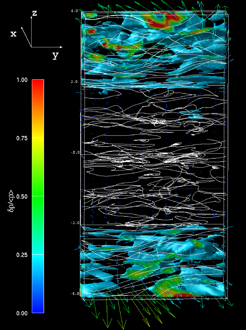
Figure 1.— Snapshot of the local disk structure at $t=210$ rotations. The white solid lines are magnetic fields, the arrows indicate velocity fields, and the colored region corresponds to $\delta\rho/{\langle\rho\rangle}>0$.

In most of the simulation region, the initial magnetic fields are moderately weak, so it is unstable with respect to MRI. In $|z|<2.5H_{0}$, however, we cannot initially resolve the wavelengths, $\lambda_{\rm max}\approx 2\pi v_{\rm A}/\Omega_{0}$, of the most unstable mode because $\lambda_{\rm max}<\Delta z(=H_{0}/32)$, where $v_{\rm A}=B/\sqrt{4\pi\rho}$ is Alfvén speed and $\Delta z$ is the mesh size (the initial $\lambda_{\rm max}\approx 0.2\Delta z$ at the midplane). First, MRI develops around $z\approx\pm 3H_{0}$ after $\approx 3$ rotations. The turbulence driven by MRI gradually spreads toward the midplane, since the growth time (approximately $\propto\Delta z/\lambda_{\rm max}$ for $\Delta z>\lambda_{\rm max}$) of the resolved wavelength is longer there. When $t\gtrsim 100$ rotations, the midplane finally becomes turbulent. The magnetic field strength saturates in the entire box after $t\gtrsim 200$ rotations, and the system becomes quasi-steady-state. At this time, $\lambda_{\rm max}$ can be resolved even at the midplane owing to the increase of the field strength. We continue the simulation further up to 400 rotations.

Figure 1 is the snapshot of magnetic field (white lines), velocity field (arrows), and $\delta\rho/{\langle\rho\rangle}$ (color) at $t=210$ rotations, where ${\langle\rho\rangle}$ is the density averaging over each $x$-$y$ plane and $\delta\rho=\rho-\langle\rho\rangle$. The magnetic fields are turbulent, dominated by the toroidal ($y$) component because of winding. Angular momentum is outwardly transported by anisotropic stress due to the MHD turbulence. At the saturated state, $\alpha\equiv(v_{x}\delta v_{y}-\frac{B_{x}B_{y}}{4\pi\rho})/c_{s}^{2}$ is $\sim 0.01$ in the midplane. One can also observe that the structured outflows stream out from both the upper and lower boundaries. Below we inspect the properties of the outflows in more detail.

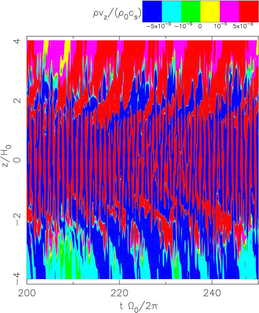
Figure 2.— Time-height diagram of the mass flux, $\rho v_{z}$, normalized by $\rho_{0}c_{s}$. $\rho v_{z}$ is averaged on the $x$-$y$ plane at each height, $z$ (vertical axis). The unit of of horizontal axis is the rotation period ($2\pi/\Omega_{0}$).

Figure 2 presents the mass flux of the $z$-component, $\rho v_{z}/\rho_{0}c_{s}$, in the $t-z$ plane. We averaged $\rho v_{z}$ on the $x$-$y$ plane at each $z$ grid point. One can see that the gas flows out from both the upper and lower boundaries. The mass fluxes near the surface regions are highly time dependent with a quasi-periodic cycle of $\sim 5-10$ rotations. Moreover, from $z\sim\pm 2H_{0}$ the mass fluxes direct to the midplane, almost coinciding with the periodicities of the outflow fluxes. In other words, the mass flows are ejected to both upward and downward directions from ‘injection regions’ located at $z\sim\pm 2H_{0}$.

These features are consequences of the breakup of channel flows (e.g., Sano & Inutsuka, 2001; Sano et al., 2004). At $z\sim\pm 2H_{0}$, the wavelength of the most unstable mode with respect to MRI, $\lambda_{\rm max}$, is comparable with the scale height, $H_{0}$. In the region $|z|>2H_{0}$, $\lambda_{\rm max}>H_{0}$; hence, it is stable against MRI. In the region $|z|<2H_{0}$, smaller-scale turbulence develops preferentially because $\lambda_{\rm max}<H_{0}$. Therefore, at $z\sim\pm 2H_{0}$ the largest scale channel flows develop, and their breakup by reconnections drives the mass flows to both upward and downward directions. In the region $|z|<2H_{0}$, the gas pressure largely dominates the magnetic pressure so that strong mass flows cannot be driven by the magnetic force associated with reconnections between small-scale turbulent fields. The periodic oscillation of 1 Keplerian rotation time around the midplane is the vertical (epicycle) motion.

Figure 3.— Time-averaged disk structure during $t=200$-$400$ rotations. The variables are also averaged on the $x$-$y$ plane at each $z$ grid. The top panel shows $v_{z}/c_{s}$ (solid), whereas the dotted line is the initial condition ($v_{z}/c_{s}=0$). The second panel presents density (solid; left axis) and plasma $\beta$ (dashed; right axis), in comparison with the initial condition (dotted; for both density and plasma $\beta$). The third panel presents the magnetic energy, $B^{2}/4\pi$. The dashed, solid, and dotted lines correspond to the $x$-, $y$-, and $z$-components, and the $y$-component shows both mean (thick) and fluctuation (thin) components. The bottom panel illustrates the energy flux in units of $\rho_{0}(H_{0}\Omega)^{3}$. The solid and dotted lines are the Poynting flux associated with the magnetic tension ($-B_{z}\delta v_{\perp}B_{\perp}/4\pi$) and the magnetic energy ($B_{\perp}^{2}v_{z}/4\pi$). The dot-dashed line is the net energy flux due to sound waves ($\delta\rho\delta v_{z}c_{s}^{2}$: see the text). The dashed line is the term concerning the potential energy ($\rho v_{z}\Phi$). The circles are the ‘injection regions’ defined as the locations where the signs of $-B_{z}\delta v_{\perp}B_{\perp}/4\pi$ change.

Figure 3 presents the disk wind structure averaged over 200 - 400 rotations. The variables are averaged on the $x$-$y$ plane at each $z$ point. The top panel shows that the average outflow velocity is nearly the sound speed at the upper and lower surfaces. The second panel presents the structures of density and plasma $\beta$ value. The comparison of the final density structure (solid) with the initial hydrostatic structure (dotted) shows that the mass is loaded up to the onset regions of outflows from $z\approx\pm 2H_{0}$. In the wind region $|z|\gtrsim 3H_{0}$, $\beta$ is below unity; the disk winds start to accelerate when the magnetic pressure dominates the gas pressure.

The third panel shows magnetic energy at the saturated state. The dashed, solid, and dotted lines are $x$-, $y$-, and $z$-components, respectively. In the $y$-component we show both mean, $\langle B_{y}\rangle^{2}$ and fluctuation, $\delta B_{y}^{2}$, components. $\langle B_{y}\rangle^{2}$ is the simple average on the $x$-$y$ planes, $\langle B_{y}(z)\rangle=\int\int dxdyB_{y}(x,y,z)/(L_{x}L_{y})$, and the fluctuations are determined from $\delta B_{y}^{2}(z)=\int\int dxdy(B_{y}(x,y,z)-\langle B_{y}(z)\rangle)^{2}/(L_{x}L_{y})$, where $L_{x}(=H_{0})$ and $L_{y}(=4H_{0})$ are the $x$ and $y$ lengths of the simulation box. As for $B_{x}$ and $B_{z}$ the fluctuation components greatly dominate the means. The magnetic energy, which is dominated by the toroidal ($y$) component as a consequence of winding, is amplified by $\approx$ 1000 times of the initial value ($B_{z,0}^{2}/4\pi=10^{-6}$) in most of the region ($|z|<3H_{0}$). While in the region near the midplane ($|z|<1.5H_{0}$), the magnetic field is dominated by the fluctuating component ($\delta B_{y}$), the mean component dominates in the regions near the surfaces ($|z|>1.5H_{0}$). In the surface regions the magnetic pressure is comparable to or larger than the gas pressure ($\beta\lesssim 1$), and so, the gas motions cannot control the configuration of the magnetic fields. Therefore, the field lines tend to be straightened by magnetic tension to give $\langle B\rangle^{2}>\delta B^{2}$ there, even if the gas is turbulent. We also note that $\langle B_{z}^{2}\rangle$ is amplified by MRI and Parker (1966) instability, whereas $\langle B_{z}\rangle^{2}$ is strictly conserved.

The bottom panel shows the status of energy transfer. The $z$-component of the total energy flux is expressed as

$$\rho v_{z}\left(\frac{1}{2}v^{2}+\Phi+h\right)+v_{z}\frac{B_{\perp}^{2}}{4\pi}-\frac{B_{z}}{4\pi}(v_{\perp}B_{\perp}),$$ (1)

where $h$ is the enthalpy, $\Phi=z^{2}/2$, and $\perp$ denotes $x$ and $y$; e.g. $B_{\perp}^{2}=B_{x}^{2}+B_{y}^{2}$. The Poynting flux is separated from the term of direct transport of magnetic energy ($B_{\perp}^{2}v_{z}/4\pi$) and the term related to magnetic tension ($-B_{z}v_{\perp}B_{\perp}/4\pi$). The solid and dotted lines are respectively $-B_{z}\delta v_{\perp}B_{\perp}/4\pi$ and $B_{\perp}^{2}v_{z}/4\pi$, where $\delta v_{\perp}=v_{x}$ and $v_{y}+3/2\Omega_{0}x$ ($-3/2\Omega_{0}x$ is the background Kepler rotation). The dashed line is the potential energy term, $\rho v_{z}\Phi$. The dot-dashed line is the energy flux of sound waves, $\delta\rho\delta v_{z}c_{s}^{2}$ (see below). The gas pressure ($pv_{z}$) and hydrodynamical turbulent pressure ($\rho\delta v^{2}v_{z}/2$) are smaller than these terms. The kinetic energy flux of the winds ($\frac{1}{2}\rho v_{z}^{3}$) is also small $\lesssim 10^{-5}$ at the outer boundaries.

The figure shows that the materials near the surfaces are lifted up by the conversion of the Poynting flux; the absolute values of the Poynting flux terms (solid and dotted) decrease with height in the region $|z|\gtrsim 2H_{0}$, and the absolute value of the potential energy flux (dashed) increases. Both magnetic pressure and tension terms contribute almost equally.

$-B_{z}\delta v_{\perp}B_{\perp}/4\pi$ and $\delta\rho\delta v_{z}c_{s}^{2}$ are the net energy fluxes of Alfvén waves and sound waves to the $+z$-direction. $-B_{z}\delta v_{\perp}B_{\perp}/4\pi$ can be rewritten as

$$-\frac{1}{4\pi}B_{z}\delta v_{\perp}B_{\perp}=\rho v_{{\rm A},z}(\delta v_{\perp,+}^{2}-\delta v_{\perp,-}^{2}),$$ (2)

where $v_{{\rm A},z}=B_{z}/\sqrt{4\pi\rho}$, and $\delta v_{\perp,\pm}=\frac{1}{2}(\delta v_{\perp}\mp B_{\perp}/\sqrt{4\pi\rho})$ are Elsässer variables, which correspond to the amplitudes of Alfvén waves propagating to the $\pm z$-directions. $\delta\rho\delta v_{z}c_{s}^{2}$ is also rewritten as

$$\delta\rho\delta v_{z}c_{s}^{2}=\rho c_{s}(\delta v_{\parallel,+}^{2}-\delta v_{\parallel,-}^{2}),$$ (3)

where $\delta v_{\parallel,\pm}=\frac{1}{2}(\delta v_{z}\pm c_{s}\frac{\delta\rho}{\rho})$ denote the amplitudes of sound waves propagating in the $\pm z$-directions.

An interesting feature of $-B_{z}\delta v_{\perp}B_{\perp}/4\pi$ is that the sign changes at $z\approx\pm 1.6H_{0}$ (the circles in the bottom panel); in $z>1.6H_{0}(<-1.6H_{0})$, the flux is upward (downward) and $|z|<1.6H_{0}$ the flux is toward the midplane. This is a consequence of the breakup of channel flows, as described previously. Reconnections break up channel flows and generate large amplitude ($|\delta{B_{\perp}}|>|B_{z}|$) Alfvén(ic) waves in both upward and downward directions. $\delta\rho\delta v_{z}c_{s}^{2}$ is also directed to the midplane, namely sound(-like) waves are generated by the reconnections. The absolute value of the energy flux peaks at the injection regions at $z\approx\pm 1.6H_{0}$. The energy flux of sound waves to the midplane is larger than that of the Alfvén waves. On the other hand, the Alfvén wave component greatly dominates in the flux to the surfaces. This is because $\beta>1$ (the gas pressure dominates) in $|z|\lesssim 2H_{0}$ and $\beta\lesssim 1$ near the surfaces.

Figure 4.— Dependence of the final $\beta$ structure on initial magnetic fields. The dash-dot-dotted, dot-dashed, dotted, solid, and dashed lines correspond to the initial vertical fields with $\beta_{0}=10^{4},10^{5},10^{6}$, and $10^{7}$, and the initially toroidal field cases. The arrows indicate the locations of the injection regions defined as the points where the sings of $-B_{z}\delta{v}_{\perp}B_{\perp}$ change. Longer arrows correspond to smaller $\beta_{0}$ (the shortest arrows are for the initially toroidal case).

Figure 5.— Sum of the mass fluxes normalized by $\rho_{0}c_{s}$ of the disk winds from the top and bottom boundaries of the simulation box. The horizontal axis indicates the initial $\beta_{0}$ at the midplane for the vertical field cases circles. The initially toroidal case is plotted at the leftmost location (triangle).

In order to study the effects of the initial magnetic fields, we performed the simulations with initial different vertical field strengths, $\beta_{0}=10^{4},10^{5},10^{6},10^{7}$, and initially toroidal field in $|z|<3H_{0}$ with $\beta_{0}=10^{6}$ at the midplanes. Figure 4 compares $\langle\beta\rangle$ structures. Figure 5 compares the sum of disk mass fluxes from the upper and lower boundaries with various cases for the initial $\beta_{0}$ at the midplane. In all cases except the $\beta_{0}=10^{4}$ case, we averaged the variables during 200 rotations after the quasi-steady-states are achieved. For the $\beta_{0}=10^{4}$ case, we show the time averages during 25-55 rotations because the quasi-steady-state is not achieved but 90 % of the total mass escapes at 75 rotations as a result of the effective mass loss by disk winds.

All the cases of $\beta_{0}\geq 10^{5}$ show very similar $\langle\beta\rangle$ structures (Figure 4): $\beta\approx 100$ at the midplanes, namely the magnetic energy can be amplified to $\approx 1$% of the gas energy. The $\beta$ values decrease with increasing height mainly because of the decrease of the densities (the magnetic energies stay nearly constant; Figure 3). When the magnetic energy dominates ($\beta\lesssim 1$), the disk winds start to accelerate. In the wind regions, the $\beta$ values stay at $\beta=0.1$-$1$, rather than further decrease, owing to the increased density by the lift-up gas in the winds. The locations of the injection regions also concentrate at $|z|/H_{0}=1.5$-$2$ except for the initial $\beta_{0}=10^{4}$ case. The plasma $\beta$ values of the injection regions are 1-10; the magnetic energy is comparable to but slightly smaller than the equipartition value. This condition is favorable for driving mass motions by the breakup of large-scale channel flows; if the magnetic energy is larger, the field configuration becomes more coherent due to the tension so that reconnections hardly occur; if the magnetic energy is smaller, the reconnections cannot drive strong mass motion. The mass flux of the disk winds (Figure 5) only weakly depends on $\beta_{0}$ for $\beta_{0}\geq 10^{6}$, while it increases for smaller $\beta_{0}$ almost in proportion with $\beta_{0}$.

4. Discussions

We have shown that the gas is lifted up from the injection regions at $|z|/H_{0}\approx 1.5$-$2$ to the surfaces by the Poynting flux and streams out from the upper and lower boundaries of the simulation box. In effect, our results determine the condition of “mass loading” in various models of global disk wind (e.g., Blandford & Payne, 1982; Kudoh & Shibata, 1997, Ferreira et al 2006), in which one usually fixes the mass flux in advance by setting the densities at the ‘bases’ of winds. With our outgoing boundary condition, we implicitly assume that once the gas goes out of the $z$-boundaries of the simulation box it does not return. The validity of this treatment needs to be examined by the global modeling of accretion disks.

Although in the shearing box treatment the time-averaged net mass flow in the $x$-direction is zero, we can estimate the accretion velocity, $-v_{r}\approx\alpha c_{s}^{2}/r\Omega_{0}$, from the angular momentum balance under steady states, where $r$ is a cylindrical distance from a central star (Shakura & Sunyaev, 1973). The ratio of the mass-loss rate, $\dot{M}_{z}$, from the simulation box by the disk winds to the mass accretion rate, $\dot{M}_{r}$, passing through the $y$-$z$ plane becomes

$$\frac{\langle\dot{M}_{z}\rangle}{\langle\dot{M}_{r}\rangle} \approx \frac{\int\int dxdy\langle\rho v_{z}\rangle}{\int dy\langle\Sigma\bar{\alpha}\rangle c_{s}^{2}/(r\Omega_{0})}=\frac{\langle\langle\rho v_{z}\rangle\rangle{L_{x}}r\Omega_{0}}{\langle\langle\Sigma\bar{\alpha}\rangle\rangle c_{s}^{2}}$$ (4)

$$\approx 0.05\left(\frac{r}{10H_{0}}\right)\left(\frac{L_{x}}{H_{0}}\right),$$

where $\Sigma=\int dz\rho$ and $\bar{\alpha}=\int dz\rho\alpha/\Sigma$; $\langle\rangle$ denotes the time-average and $\langle\langle\rangle\rangle$ is the average of time and $x$-$y$ planes. The final value is estimated from $\langle\langle\rho v_{z}\rangle\rangle\approx 8\times 10^{-5}\rho_{0}c_{s}$ and $\bar{\alpha}\approx 0.012$ in our fiducial run for a moderately thin disk with $H_{0}/r=0.1$. We should take the above estimate as an upper limit because the calculation with a larger vertical box size may give a smaller mass flux at the top and bottom boundaries. The angular momentum loss rates in vertical and radial directions give the same scaling,

$$\frac{\langle\dot{\cal{L}}_{z}\rangle}{\langle\dot{\cal{L}}_{r}\rangle}=\frac{\int\int dxdy\langle\rho v_{z}\rangle r^{2}\Omega_{0}}{\int dyr\langle\Sigma\bar{\alpha}\rangle c_{s}^{2}}=\frac{\langle\langle\rho v_{z}\rangle\rangle L_{x}r\Omega_{0}}{\langle\langle\Sigma\bar{\alpha}\rangle\rangle c_{s}^{2}}\approx\frac{\langle\dot{M}_{z}\rangle}{\langle\dot{M}_{r}\rangle},$$ (5)

because the time-averaged specific angular momentum carried by the winds is approximately the same as that in the disk material at the same radial position in the shearing box treatment. In a realistic situation, however, winds possibly carry a larger specific angular momentum than the disk material. For such studies, we need to model global accretion disks with disk winds, which is also important from the viewpoint of angular momentum evolution of the star-disk system (e.g. Matt & Pudritz, 2005).

Hereafter we discuss the evolution of protoplanetary disks, as an application of our results. As a reference model, we use the minimum-mass solar nebula (MMSN) of Hayashi (1981), which gives the midplane density, $\rho_{0}=1.4\times 10^{-9}\left(\frac{r}{\rm 1AU}\right)^{-11/4}{\rm g\;cm^{-3}}$. Then, the initial vertical magnetic field of $\beta_{0}=10^{6}$ in our fiducial run corresponds to $B_{z,0}\approx 0.01$ G, and the saturated field strength is $B\approx 1$ G at 1 AU.

First, we examine how much the disk wind contributes to the evaporation of protoplanetary disks (see e.g. Dullemond et al., 2007, for other mechanisms). After the saturation of the magnetic fields, $\approx 5$% of the total disk mass is lost from the simulation box from 200 to 400 rotations by the disk winds in our fiducial case. Assuming a disk around a central star with the solar mass (1 rotation = 1 yr at 1 AU), we have the timescales of the evaporation, $\tau_{\rm ev}\approx 4000$ yr at 1 AU, and $6\times 10^{5}$ yr at 30 AU. Although this is rather short in comparison with recent observational results (typically $\tau_{\rm ev}\sim 10^{6-7}$ yrs, e.g., Haisch, Lada, & Lada, 2001), this is not a severe contradiction because we have not yet taken into account the global radial accretion of the disk mass, which continuously supplies the mass from the outer region. Another important issue that affects, and might reduce, the mass flux of disk winds is the effect of resistivity, which requires an additional detailed analysis of the ionization structure (Sano et al., 2000; Inutsuka & Sano, 2005) and will be the scope of our next paper. Here, the estimated $\tau_{\rm ev}$ should be taken as a lower limit.

The disk scale height has a relation of $H_{0}/r\propto r^{1/4}$ for the MMSN. Combining with Equation (4), we infer that the dynamical evaporation by disk winds, in comparison with accretion, becomes relatively more important in the inner parts of protoplanetary disks than in the outer regions for a constant initial $\beta_{0}$ structure ($B_{z,0}^{2}\propto r^{-11/4}$ for the MMSN).

Finally, we should point out the effects of waves on dusts in protoplanetary disks. We have shown that the momentum flux of Alfvènic and sound-like waves directs to the midplane from the injection regions. The momentum flux of the sound-like waves ($\delta\rho\delta v_{z}$) can push dust grains to the midplane by gas-dust collisions. Dusts are usually weakly charged; in this case Alfvénic waves also contribute to the sedimentation of dusts to the midplane through ponderomotive force or dust-cyclotron resonance (Vidotto & Jatenco-Pereira, 2006).

This work was supported in part by Grants-in-Aid for Scientific Research from the MEXT of Japan (T.K.S.: 19015004 and 20740100, S.I.: 15740118, 16077202, and 18540238), and Inamori Foundation (T.K.S.). Numerical computations were in part performed on Cray XT4 at Center for Computational Astrophysics, CfCA, of National Astronomical Observatory of Japan. The page charge of this paper is supported by CfCA.

References

- Balbus & Hawley (1991) Balbus, S. A. & Hawley, J. F. 1991, ApJ, 376, 214
- Blandford & Payne (1982) Blandford, R. D. & Payne, D. G. 1982, MNRAS, 199, 883
- Brandenburg et al. (1995) Brandenburg, A., Nordlund, øA., Stein, R., & Torkelsson, U. 1995, ApJ, 446, 741
- Clarke (1996) Clarke, D. A. 1996, ApJ, 457, 291
- Dullemond et al. (2007) Dullemond, C. P., Hollenbach, D., Kamp, I., & D’Alessio, P. 2007, Protostars & Planets V, B. Reipurth, D. Jewitt, and K. Keil, eds., Univ. of Arizona Press, 951, 555
- Ferreira, Dougados & Cabrit (2006) Ferreira, J., Dougados, C., & Cabrit, S. 2006, A&A, 453, 785
- Haisch, Lada, & Lada (2001) Haisch, K. E. Jr., Lada, E. A., & Lada, C. A. 2001, ApJ, 553, 153
- Hawley, Gammie, & Balbus (1995) Hawley, J. F., Gammie, C. F. & Balbus, S. A. 1995, ApJ, 440, 742
- Hayashi (1981) Hayashi, C. 1981, Prog. Theoretical Phys. Supp., 70, 35
- Inutsuka & Sano (2005) Inutsuka, S. & Sano, T. 2005, ApJ, 628, L155
- Kudoh & Shibata (1997) Kudoh, T. & Shibata, K. 1997, ApJ, 474, 362
- Matt & Pudritz (2005) Matt, S. & Pudritz, R. E. 2005, ApJ, 632, L135
- Miller & Stone (2000) Miller, K. A. & Stone, J. M. 2000, ApJ, 534, 398
- Parker (1966) Parker, E. N. 1966, ApJ, 145, 811
- Sakao et al. (2007) Sakao, T. et al. 2007, Science, 318, 1585
- Sano et al. (2000) Sano, T., Miyama, S. M., Umebayashi, T., & Nakano, T. 2000, ApJ, 543, 486
- Sano & Inutsuka (2001) Sano, T. & Inutsuka, S., 2001, ApJ, 561, L179
- Sano et al. (2004) Sano, T., Inutsuka, S., Turner, N. J., & Stone, J. M. 2004, ApJ, 605, 321
- Shakura & Sunyaev (1973) Shakura, N. I. & Sunyaev, R. A. 1973, A&A, 24, 337
- Stone et al. (1996) Stone, J. M., Hawley, J. F., Gammie, C. F., & Balbus, S. A. 1996, ApJ, 463, 656
- Suzuki (2007) Suzuki, T. K. 2007, ApJ, 659, 1592
- Suzuki & Inutsuka (2005) Suzuki, T. K. & Inutsuka, S. 2005, ApJ, 632, L49 (SI05)
- Suzuki & Inutsuka (2006) —— 2006, J. Geophys. Res., 111, A6, A06101
- Thompson (1987) Thompson, K. W. 1987, J. Comp. Phys., 68, 1
- Tsuneta et al. (2008) Tsuneta, S. et al. 2008, ApJ, in press (arxiv:0807.4631)
- Turner & Sano (2007) Turner, N. J. & Sano, T. 2007, ApJ, 659, 729
- Vidotto & Jatenco-Pereira (2006) Vidotto, A. A. & Jatenco-Pereira, V. 2006, ApJ, 639, 416