Metallic ferromagnetism in the Kondo lattice

Abstract

Metallic magnetism is both ancient and modern, occurring in such familiar settings as the lodestone in compass needles and the hard drive in computers. Surprisingly, a rigorous theoretical basis for metallic ferromagnetism is still largely missing. The Stoner approach perturbatively treats Coulomb interactions when the latter need to be large, while the Nagaoka approach incorporates thermodynamically negligible holes into a half-filled band. Here, we show that the ferromagnetic order of the Kondo lattice is amenable to an asymptotically exact analysis over a range of interaction parameters. In this ferromagnetic phase, the conduction electrons and local moments are strongly coupled but the Fermi surface does not enclose the latter (i.e., it is “small”). Moreover, non-Fermi liquid behavior appears over a range of frequencies and temperatures. Our results provide the basis to understand some long-standing puzzles in the ferromagnetic heavy fermion metals, and raise the prospect for a new class of ferromagnetic quantum phase transitions.

A contemporary theme in quantum condensed matter physics concerns competing ground states and the accompanying novel excitations Coleman05 . With a plethora of different phases, magnetic heavy fermion materials should reign supreme as the prototype for competing order. So far, most of the theoretical scrutiny has focused on antiferromagnetic heavy fermions Gegenwart08 ; HvL07 . Nonetheless, the list of heavy fermion metals which are known to exhibit ferromagnetic order continues to grow. An early example subjected to extensive studies is CeRu₂Ge₂ (ref. Sullow99 and references therein). Other ferromagnetic heavy fermion metals include CePt Larrea05 , CeSi_x Drotziger06 , CeAgSb₂ Sidorov03 , and URu_2-xRe_xSi₂ at ${\rm x}>0.15$ Bauer05 ; Butch09 . More recently discovered materials include CeRuPO Krellner07 and UIr₂Zn₂₀ Bauer06 . Finally, systems such as UGe₂ Saxena00 and URhGe Levy07 are particularly interesting because they exhibit a superconducting dome as their metallic ferromagnetism is tuned toward its border. Some fascinating and general questions have emerged King91 ; Yamagami94 ; Ikezawa97 , yet they have hardly been addressed theoretically. One central issue concerns the nature of the Fermi surface: Is it “large,” encompassing both the local moments and conduction electrons as in paramagnetic heavy fermion metals Hewson97 ; Oshikawa00 , or is it “small,” incorporating only conduction electrons? Measurements of the de Haas-van Alphen (dHvA) effect have suggested that the Fermi surface is small in CeRu₂Ge₂ King91 ; Yamagami94 ; Ikezawa97 , and have provided evidence for Fermi surface reconstruction as a function of pressure in UGe₂ Settai02 ; Huxley . At the same time, it is traditional to consider the heavy fermion ferromagnets as having a large Fermi surface when their relationship with unconventional superconductivity is discussed Saxena00 ; Levy07 ; Schofield03 ; an alternative form of the Fermi surface in the ordered state could give rise to a new type of superconductivity near its phase boundary. All these point to the importance of theoretically understanding the ferromagnetic phases of heavy fermion metals, and this will be the focus of the present work.

We consider the Kondo lattice model in which a periodic array of local moments interact with each other and with a conduction-electron band. Kondo lattice systems are normally studied in the paramagnetic state, where Kondo screening leads to heavy quasiparticles in the single-electron excitation spectrum Hewson97 . The Stoner Stoner38 mean field treatment of these heavy quasiparticles may then lead to an itinerant ferromagnet Perkins07 . With the general limitations of the Stoner approach in mind, here we carry out an asymptotically exact analysis of the ferromagnetic state. We are able to do so by using a reference point that differs from either the Stoner or Nagaoka approach Nagaoka66 , and accessing a ferromagnetic phase whose excitations are of considerable interest in the context of heavy fermion ferromagnets. We should stress that a ferromagnetic order may also arise in different regimes of related models, such as in one dimension Sigrist92 or in the presence of mixed-valency Batista03 .

Our model contains a lattice of spin-$\frac{1}{2}$ local moments (${\bf S}_{i}$ for each site $i$) with a ferromagnetic exchange interaction ($I<0$), a band of conduction electrons ($c_{{\vec{K}}\sigma}$, where ${\vec{K}}$ is the wavevector and $\sigma$ the spin index) with a dispersion $\epsilon_{\vec{K}}$ and a characteristic bandwidth $W$, and an on-site antiferromagnetic Kondo exchange interaction ($J_{K}>0$) between the local moments and the spin of the conduction electrons. The corresponding Hamiltonian is

$$H=\sum_{{\vec{K}}}\epsilon^{\phantom{\dagger}}_{\vec{K}}c^{\dagger}_{{\vec{K}}\sigma}c^{\phantom{\dagger}}_{{\vec{K}}\sigma}+I\sum_{\langle ij\rangle}S_{i}^{a}S_{j}^{a}+\sum_{i}J_{K}^{a}S_{i}^{a}c^{\dagger}_{i\sigma}\frac{\tau^{a}_{\sigma\sigma^{\prime}}}{2}c^{\phantom{\dagger}}_{i\sigma^{\prime}}.$$ (1)

The symbol $\tau$ represents the Pauli matrices, with indices $a\in\{x,y,z\}$ and $\sigma\in\{\uparrow,\downarrow\}$. Here $I$ represents the sum of direct exchange interaction between the local moments and the effective exchange interaction generated by the conduction electron states that are not included in Eq. (1). Incorporating this explicit exchange interaction term allows the study of the global phase diagram of the Kondo lattice systems, and tuning a control parameter in any specific heavy fermion material represents taking a cut within this phase diagram. The Hamiltonian above is to be contrasted with models for double-exchange ferromagnets in the context of, for example, manganites, where it is the “Kondo” coupling that is ferromagnetic due to Hund’s rule.

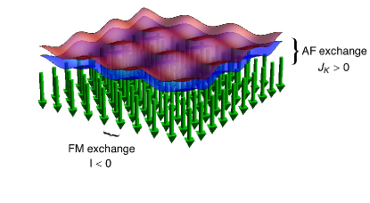
Figure 1: An illustration of the Kondo lattice. Local moments from f-orbitals are in green, and are depicted here to be spin down. Spin-up conduction electrons are in red, which have a higher probability density than the spin-down conduction electrons in blue. The Hamiltonian for the model is given in Eq. (1) where $\sigma$ is the spin index and $a$ refers to the three spin directions. Note that the Einstein summation convention is used on indices. For simplicity, we assume $\epsilon_{\vec{K}}=\frac{K^{2}}{2m_{e}}$. The characteristic kinetic energy, $W$, is defined as $W\equiv 1/\rho_{0}$, where $\rho_{0}\equiv\sum_{\vec{K}}\delta(E_{F}-\epsilon_{\vec{K}})$ is the single-particle density of states at the Fermi energy ($E_{F}$). Both $E_{F}$ and the chemical potential, $\mu$, scale like $W$. We use the Shankar notation with $K=|\vec{K}|$ measured from the center of the Brillouin zone.

The parameter region we will focus on is $J_{K}\ll|I|\ll W$. Here we can use the limit $J_{K}=0$ as the reference point, which contains the local moments, representing the f-electrons with strong repulsions, and conduction electrons. As illustrated in Fig. 1, the local moments order in a ferromagnetic ground state because $I<0$, whereas the conduction electrons form a Fermi sea with a Fermi surface. A finite but small $J_{K}$ will couple these two components, and its effect is analyzed in terms of a fermion$+$boson renormalization group (RG) procedure  Yamamoto07 ; Altshuler94 ; Shankar90 . We will use an effective field theory approach, which we outline below and describe in detail in the Supporting Information. Though our analysis will focus on this weak $J_{K}$ regime, the results will be germane to a more extended parameter regime through continuity.

The Heisenberg part of the Hamiltonian, describing the local moments alone, is mapped to a continuum field theory Read95 in the form of a Quantum Nonlinear Sigma Model (QNL$\sigma$M). In this framework, the local moments are represented by an O(3) field, $\vec{m}$, which is constrained non-linearly with a continuum partition function. Combining the local moments with the conduction electrons, we reach the total partition function: $Z=\int\mathcal{D}\vec{m}\mathcal{D}[\bar{\psi},\psi]\;\delta(\vec{m}^{2}(\vec{x},\tau)-1)e^{-\mathcal{S}}$, where $\mathcal{S}=\mathcal{S}_{m}+\mathcal{S}_{c}^{\prime}+\mathcal{S}_{K}$. The action for the conduction electrons, $\mathcal{S}_{c}^{\prime}$, is standard. Defining $m^{+}=m_{x}+im_{y}$ and $m^{-}=m_{x}-im_{y}$, the low energy action for the local moments is expressed in terms of a single complex scalar:

$$\mathcal{S}_{m} \approx \frac{1}{2}\int d\omega d^{d}q\;m^{+}(\vec{q},i\omega)(-M_{0}i\omega+\rho_{s}q^{2})m^{-}(-\vec{q},-i\omega)$$ (2)

$$+g\int\left(\partial m\right)^{4}$$

Here, $M_{0}$ is the magnetization density, and $\rho_{s}$ the magnon stiffness constant. The magnon-magnon coupling $g$, schematically written above and more precisely specified in the Supporting Information, turns out to be irrelevant in the RG sense when fermions are also coupled to the system. This 4-boson term, involving four gradients, was found to be relevant for $d>2$ in a model without fermions Read95 but is unimportant when fermions are part of the system, as in our model here. Finally, the Kondo coupling can be separated into static and dynamic parts. The static order of the local moments induces a splitting of the conduction electron band on the order of $\Delta\sim J_{K}^{z}\langle m^{z}\rangle\sim J_{K}^{z}$, which modifies $\mathcal{S}_{c}^{\prime}$ into the following action for the conduction electrons

$$\mathcal{S}_{c}=\int d^{d}Kd\epsilon\;\bar{\psi}_{\sigma}(\vec{K},\epsilon)\left(-i\epsilon+\frac{K^{2}}{2m_{e}}-\mu+\sigma\Delta\right){\psi}_{\sigma}(\vec{K},\epsilon)$$

The dynamical part couples the magnons with the conduction electrons, leading to

$$\mathcal{S}_{K}^{\pm} = J_{K}^{\pm}\int d^{d}qd\omega d^{d}Kd\varepsilon\Big{(}\psi_{K+q,\uparrow}^{\dagger}\psi_{K,\downarrow}^{\phantom{\dagger}}m^{-}_{q}$$ (4)

$$+\quad\psi_{K+q,\downarrow}^{\dagger}\psi_{K,\uparrow}^{\phantom{\dagger}}m^{+}_{q}\Big{)}$$

$$\mathcal{S}_{K}^{z} = -\frac{J_{K}^{z}}{2}\int d^{d}q_{1}d\omega_{1}d^{d}q_{2}d\omega_{2}d^{d}Kd\varepsilon$$ (5)

$$\times\Big{(}\psi_{K+q_{1}-q_{2},\sigma}^{\dagger}\tau^{z}_{\sigma\sigma^{\prime}}\psi_{K,\sigma^{\prime}}^{\phantom{\dagger}}m^{-}_{q_{1}}m^{+}_{q_{2}}\Big{)}$$

The mapping from the microscopic model in Eq. (1) to the field theory in (2)-(5) is similar to the antiferromagnetic case Yamamoto07 , but differs from the latter in several important ways. One simplification is that the translational symmetry is preserved in the ferromagnetic phase. At the same time, two complications arise. Ferromagnetic order breaks time-reversal symmetry, which is manifested in the Zeeman splitting of the spin up and down bands. In addition, the effective field theory for a local-moment quantum ferromagnet involves a Berry phase term Read95 such that Lorentz invariance is broken, even in the continuum limit; the dynamic exponent, connecting $\omega$ and $q$ in Eq. (2), is $z=2$ instead of $1$. The effective field theory, comprising Eqs. (2)-(5), is subjected to a two-stage RG analysis as detailed in the Supporting Information.

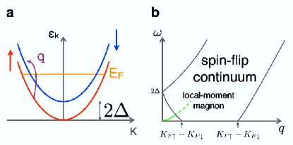
Figure 2: Phase space for the Kondo coupling. a, The spin-splitting of the conduction electron band, which kinematically suppresses interband processes associated with the Kondo spin-flip coupling to the local-moment magnons. b, The kinematics for the spin-flip Kondo coupling. The low-lying excitations of the local-moment system are the magnons which enter the continuum at finite $\omega$ and $q$. Those of the conduction electrons are expressed in terms of the spin-flip continuum, whose Kondo-coupling to the local-moment magnons is cut off below the cutoff energy, $\omega_{c}\approx(I/W^{2})\Delta^{2}$, and the cutoff momentum, $q_{c}\approx K_{F\uparrow}-K_{F\downarrow}\approx(K_{F}/W)\Delta$.

I Results

For energies and momenta above their respective cutoffs, $\omega_{c}\sim(I/W^{2})\Delta^{2}$ and $q_{c}\sim(K_{F}/W)\Delta$, the magnons are coupled to the continuum part of the transverse spin excitations of the conduction electrons, see Fig. 2. Here, the Kondo coupling is relevant in the RG sense below three dimensions. This implies strong coupling between the conduction electrons and the local moments, and both the QNL$\sigma$M as well as the action for the conduction electrons will be modified. Explicitly, the correction to the quadratic part of the QNL$\sigma$M is

$$\Pi(\vec{q},\omega)\approx J_{K}^{2}\rho_{0}\left(1+i\gamma\frac{\omega}{v_{F}q}\right)$$ (6)

where $\gamma$ is a dimensionless constant prefactor. At the same time, the conduction electrons acquire the following self-energy:

$$\Sigma(K_{F},\epsilon) = \left\{\begin{array}[]{cc}-A_{2}(\rho_{0}J_{K}^{4}/I^{2})^{1/3}~{}(-i\epsilon)^{2/3}&~{}~{}d=2\\ -A_{3}(\rho_{0}J_{K}^{2}/I)~{}\epsilon\log(-i\epsilon)&~{}~{}d=3\end{array}\right.$$ (9)

where $A_{2}$ and $A_{3}$ are dimensionless constants of order unity. The self energies $m^{+}\Pi m^{-}$ and $\bar{\psi}\Sigma\psi$ add directly to the quadratic parts of the action, $\mathcal{S}_{m}$ and $\mathcal{S}_{c}$, respectively. Similar forms for the self-energies appear in other contexts, notably the gauge-fermion problem and the spin-fluctuation-based quantum critical regime. The formal similarities as well as some of the important differences are discussed in the Supporting Information.

With these damping corrections incorporated, the effective transverse Kondo coupling, $J_{K}^{\pm}$, becomes marginal in the RG sense in both two and three dimensions; the marginality is exact in the sense that it extends to infinite loops, as detailed in the Supporting Information. This signals the stability of the form of damping for both the magnons and conduction electrons Altshuler94 ; Polchinski93 . At the same time, the effective longitudinal Kondo coupling, $J_{K}^{z}$, as well as the non-linear coupling among the magnons, $g$, are irrelevant in the RG sense.

The exactly marginal nature of the Kondo coupling in the continuum part of the phase space implies that the effective coupling remains small as we scale down to the energy cutoff $\omega\sim\omega_{c}$ and, correspondingly, the momentum cutoff $q\sim q_{c}$. Below these cutoffs, the transverse Kondo coupling, which involves spin flips of the conduction electrons, cannot connect two points near the up-spin and down-spin Fermi surfaces; see Fig. 2. Although there is no gap in the density of states, as far as the spin-flip Kondo coupling is concerned, the system behaves as if the lowest energy excitations have been gapped out. The important conclusion, then, is that the effective transverse Kondo coupling renormalizes to zero in the zero-energy and zero-momentum limit. This establishes the absence of static Kondo screening. Hence, the Fermi surface is small, and this is illustrated in Fig. 3a.

The region of validity of Eqs. (6,9) corresponds to $\omega_{c}\ll\omega\ll|I|$ and $q_{c}\ll q\ll 2K_{F}$. This range is well-defined, given that $\Delta\approx J_{K}\langle m^{z}\rangle\leq J_{K}$ and that we are considering $J_{K}\ll|I|\ll W$. In this same energy and, correspondingly, temperature ranges, other physical properties also show a non-Fermi liquid behavior. In two dimensions, the specific heat coefficient, $C/T\sim T^{-1/3}$ and the electrical resistivity $\rho\sim T^{4/3}$. In three dimensions, $C/T\sim\log(1/T)$ and $\rho\sim T^{5/3}$. These non-Fermi liquid features have form similar to those of the quantum critical ferromagnets Smith_Nature08 ; Belitz_RMP05 , although here we are deep inside the ferromagnetically-ordered part of the phase diagram.

II Discussion

Our result is surprising given that the ratio $J_{K}/\omega_{c}\sim W^{2}/\left(IJ_{K}\langle m^{z}\rangle^{2}\right)\gg 1$. By contrast, the standard Kondo impurity problem with a pseudo-gap of order $\Delta_{pg}\ll J_{K}$ in the conduction electron density of states near the Fermi energy would be Kondo-screened Ingersent98 ; Withoff90 . The difference is that, in the latter case, the Kondo coupling renormalizes to stronger values as the energy is lowered in the range $\Delta_{pg}\ll\omega\ll W$; for $J_{K}/\Delta_{pg}\gg 1$, the renormalized Kondo coupling is already large by the time the energy is lowered to $\omega\sim\Delta_{pg}$.

The small Fermi surface we have established is to be contrasted with the large Fermi surface of a ferromagnetic heavy fermion metal in the Stoner treatment, illustrated in Fig.  3b. In the latter case, the local moments become entangled with the conduction electrons as a result of the static Kondo screening. Kondo resonances develop and the local moments become incorporated into a large Fermi surface. This Fermi surface comes from a Zeeman-splitting of an underlying Fermi surface for the paramagnetic phase; the latter is large, as seen through a non-perturbative proof Oshikawa00 that relies upon time-reversal invariance.

Figure 3: Contrasting the small and large Fermi surfaces. The spin-up electron Fermi surface is drawn in red and larger than the spin-down electron Fermi surface in blue. The larger Fermi surface has been made slightly transparent to reveal the smaller sheet. a, The local moments are not part of the Fermi surface. b, The static Kondo screening has caused the Fermi surface to expand to accommodate the Kondo resonances associated with the local moments.

Our result of a stable ferromagnetic metal phase with a small Fermi surface provides the basis to understand the dHvA-measured King91 ; Yamagami94 ; Ikezawa97 Fermi surface of CeRu₂Ge₂, which is ferromagnetic below $T_{c}=8$ K. Our interpretation rests on a dynamical Kondo screening effect that turns increasingly weak at lower energies. This is supported by the observation of the collapsing quasielastic peak measured in the inelastic neutron-scattering cross section as the temperature is reduced Rainford96 . It will be very instructive if the Fermi surface of UGe₂ Settai02 is further clarified and if systematic dHvA measurements are carried out in other ferromagnetic heavy fermion metals as well. With future experiments in mind, we note that our conclusion of a small Fermi surface also applies to ferrimagnetic order.

In the parameter regime we have considered, the non-Fermi liquid features are sizable. For instance, the non-Fermi liquid contribution to the self-energy [Eq. (9)] is, at the cutoff energy $\omega_{c}$, larger than the standard Fermi liquid term associated with the interactions among the conduction electrons. It remains to be fully established whether the non-Fermi liquid terms in the electrical resistivity and specific heat can be readily isolated from contributions of other processes. Still, there is at least one family of materials, URu_2-xRe_xSi₂ at ${\rm x}>0.15$, in which non-Fermi liquid features have been shown to persist deep inside the ferromagnetic regime Bauer05 ; Butch09 . Whether this observed feature is indeed a property of the ferromagnetic phase, or if it is related to some quantum critical fluctuations or even certain disorder effects, remains to be clarified experimentally. We hope that our theory will provide motivation for the experimental search of non-Fermi liquid behavior in ferromagnetic heavy fermion metals as well.

The existence of a ferromagnetic phase with a small Fermi surface raises the prospect of a direct quantum phase transition from a Kondo-destroyed ferromagnetic metal to a Kondo-screened paramagnetic metal. This, like its antiferromagnetic counterpart Gegenwart08 ; Paschen04 ; Park08 , in turn raises the possibility of a new type of superconductivity; the underlying quantum fluctuations would be associated with not only the development of the ferromagnetic order Saxena00 but also the transformation of a large-to-small Fermi surface. Theoretically, accessing the quantum phase transition requires that our analysis be extended to the regime where the Kondo coupling is large compared to the RKKY interaction, and this represents an important direction for the future. Experimentally, in the case of CeRu₂Ge₂, applying pressure or doping Ge with Si fails to reach a ferromagnetic-to-paramagnetic quantum phase transition due to the intervention of antiferromagnetic order; other control parameters or other ferromagnetic heavy fermions should be explored.

Finally, it is instructive to compare our study of the Kondo lattice Hamiltonian with traditional studies of itinerant ferromagnetism based on a one-band Hubbard model. We have taken advantage of the separation of energy scales of the Kondo lattice Hamiltonian and derived our results from an asymptotically exact RG analysis. By contrast, the one-band Hubbard model does not feature a separation of energy scales at the Hamiltonian level and the corresponding theoretical studies  Ueda75 have been based on mean-field (randon-phase) approximations. Furthermore, the separation of energy scales in the Kondo lattice Hamiltonian is crucial for our conclusion that the non-Fermi liquid behavior exists over a large energy window, which does not happen in the one-band case. Finally, the issue of small Fermi surface, which represents a major conclusion of our study, is absent in the case of the one-band Hubbard model.

To summarize, we have shown that the ferromagnetic Kondo lattice has a parameter range where the Kondo screening is destroyed and the Fermi surface is small. This conclusion is important for heavy fermion physics. It allows us to understand a long-standing puzzle on the Fermi surface, as epitomized by the dHvA measurements in CeRu₂Ge₂. It also sharpens the analogy with the extensively studied antiferromagnetic heavy fermion metals, where the dichotomy between Kondo breakdown and conventional quantum criticality is well established. More broadly, the present work has led to one of the very few asymptotically exact results for metallic ferromagnetism whose rigorous understanding has remained elusive for many years Vollhardt98 . Our findings highlight an important lesson, namely that correlation effects can lead to qualitatively new properties even for magnetism occurring in a metallic environment. This general lesson could very well be relevant to a broad array of magnetic systems, including the extensively-debated iron pnictides Cruz08 .

III Kondo Lattice and Field Theory

We begin with a microscopic description of heavy fermion metals in terms of the Kondo-Heisenberg Hamiltonian.

$$H = \sum_{k}\epsilon^{\phantom{\dagger}}_{\vec{K}}c^{\dagger}_{\vec{K}\sigma}c^{\phantom{\dagger}}_{\vec{K}\sigma}+I\sum_{\langle ij\rangle}S^{a}_{i}S^{a}_{j}+\sum_{i}J_{K}^{a}S^{a}_{i}c^{\dagger}_{i\sigma}\frac{\tau^{a}_{\sigma\sigma^{\prime}}}{2}c^{\phantom{\dagger}}_{i\sigma^{\prime}}$$

where $a$ labels the three spin components. For simplicity, and without loss of generality, we will consider only nearest-neighbor ($\langle ij\rangle$) ferromagnetic exchange interaction among the local moments, and we will also assume $\epsilon_{\vec{K}}=\frac{K^{2}}{2m_{e}}$. By contrast to the purely itinerant magnets, the local moments are independent degrees of freedom to begin with and, on their own, would be ferromagnetically ordered ($I<0$). These local moments are also antiferromagnetically coupled ($J_{K}>0$) to itinerant conduction electrons. The exchange interaction among the local moments includes not only the RKKY interaction generated by the conduction electrons in Eq. (III), but also the RKKY and superexchange interactions from other conduction-electron states as well as the direct exchange. We note that our model is very different from those for double-exchange ferromagnets in the context of the manganites, where the “Kondo” coupling is ferromagnetic Pandey08_SI ; Kapetanakis08_SI : there, the low-lying states are spin triplets formed by the local spins and itinerant conduction electrons, and the Kondo screening physics is never pertinent.

Since we are interested in the low energy properties of the ferromagnetic phase of this system, we adapt an effective field theory previously used for the pure quantum Heisenberg ferromagnet Read95_SI , but extend it to include fermions. Here, the spin is represented by an O(3) field, $\vec{m}$, which is constrained non-linearly.

$$Z = \int\mathcal{D}\vec{m}\mathcal{D}[\bar{\psi},\psi]\;\delta(\vec{m}^{2}(\vec{x},\tau)-1)e^{-\mathcal{S}}$$

$$\mathcal{S} \equiv \mathcal{S}_{m}^{\prime}+\mathcal{S}_{\text{Berry}}+\mathcal{S}_{c}^{\prime}+\mathcal{S}_{K}$$

$$\mathcal{S}_{m}^{\prime} = \frac{\rho_{s}}{2}\int d^{d}xd\tau\;\frac{\partial m^{a}(\vec{x},\tau)}{\partial x^{\mu}}\frac{\partial m^{a}(\vec{x},\tau)}{\partial x^{\mu}}$$

$$\mathcal{S}_{\text{Berry}} = iM_{0}\int d^{d}xd\tau\;A^{a}[\vec{m}]\frac{\partial m^{a}(\vec{x},\tau)}{\partial\tau}$$

$$\mathcal{S}_{c}^{\prime} = \int d^{d}xd\tau\;\bar{\psi}_{\sigma}(\vec{x},\tau)\left(\partial_{\tau}-\frac{\nabla^{2}}{2m_{e}}-\mu\right)\psi_{\sigma}(\vec{x},\tau)$$

$$\mathcal{S}_{K} = J_{K}^{a}\int d^{d}xd\tau\;s_{c}^{a}(\vec{x},\tau)m^{a}(\vec{x},\tau)$$ (2)

where, as usual, $s_{c}^{a}\equiv\bar{\psi}_{i\sigma}\frac{\tau^{a}_{\sigma\sigma^{\prime}}}{2}\psi_{i\sigma^{\prime}}$, and the superscript $\mu$ labels the spatial directions. The topological Berry phase term is crucial to get the dynamics right Wen88_SI . If we define the $z$-axis as the direction of magnetization, we have $\nabla_{m}\times\vec{A}=(0,0,1)=\langle\vec{m}\rangle$ (note that the curl is in field space, not real space). Thus, in a linearized, low-energy theory of spin fluctuations, we have $\vec{A}\approx(-m_{y},m_{x},0)$. Defining $m^{+}=m_{x}+im_{y}$ and $m^{-}=m_{x}-im_{y}$ we obtain a theory of a single complex scalar

$$\mathcal{S}_{m} = \mathcal{S}_{m}^{\prime}+\mathcal{S}_{\text{Berry}}$$

$$\approx \frac{1}{2}\int d\omega d^{d}q\;m^{+}(\vec{q},i\omega)\left(-M_{0}i\omega+\rho_{s}q^{2}\right)m^{-}(-\vec{q},-i\omega)$$

We have now arrived at an effective theory of local moment ferromagnetic magnons coupled to fermions with effective coupling constant that for simplicity we also label $J_{K}$. The mapping from the microscopic model in equation (III) to the field theory in (III) parallels the antiferromagnetic (AF) case Yamamoto07_SI ; Read95_SI .

IV Scaling Analysis

We need to carry out an RG analysis for the field theory above several times, both before and after self-energies have been incorporated. To begin, we summarize the pure boson problem which has been done previously Read95_SI . The dimension of the $m$ field is fixed by the nonlinear constraint $m^{a}(\vec{x},\tau)m^{a}(\vec{x},\tau)=1$ which requires $[m^{a}(\vec{x},\tau)]=0$. In momentum space, this becomes $[m^{a}(\vec{q},\omega)]=-d-z_{b}$. Unless indicated otherwise, we will exclusively be concerned with field dimensions in momentum space, so the arguments will often be dropped: $[m]=-d-z_{b}$. As usual for purely bosonic RG, the momenta and energies scale simply as $[q]=1$ and $[\omega]=z_{b}$, where $z_{b}=2$ is the dynamical exponent for the boson, which is consistent with $\omega\sim q^{2}$. The modulo $4\pi$ ambiguity in the Berry phase dictates $[M_{0}]=d$, and the scale invariance of $\mathcal{S}_{m}$ establishes $[\rho_{s}]=d+z_{b}-2$.

Read and Sachdev were the first to point out that higher order gradient terms may be relevant.

$$\mathcal{S}_{m}^{(4)} = g\int d^{d}xd\tau\Big{(}\partial_{\mu}m_{a}\partial_{\mu}m_{a}\partial_{\nu}m_{b}\partial_{\nu}m_{b}$$ (4)

$$\quad-2\partial_{\mu}m_{a}\partial_{\nu}m_{a}\partial_{\mu}m_{b}\partial_{\nu}m_{b}\Big{)}$$

Using the scaling scheme described above, this coupling, representing magnon-magnon interactions, has scaling dimension $[g]=d-2$. This indicates that, for $d>2$, the magnon-magnon scattering is relevant. We will see later why this term becomes irrelevant when fermions are incorporated.

In parallel to the pure boson problem, there is a well known procedure for handling pure fermion problems within a momentum shell approach Shankar94_SI . The essential difference from the bosonic RG is that the low energy manifold now consists of an extended surface, the Fermi surface, rather than a single point. Scaling should therefore be done with respect to this surface, and this may be accomplished by a clever change of coordinates for a simple spherical Fermi surface.

When the action contains both bosons and fermions, the momentum shell RG becomes much more complicated. In the special case $z_{f}=1$ and $z_{b}=1$, we have extended Shankar’s approach in a straightforward fashion Yamamoto07_SI . However, such an approach does not work if $z_{f}\neq z_{b}$. Another strategy has been proposed by Altshuler, Ioffe, and Millis Altshuler94_SI , and we adopt this method here. For further details on this method, see Yamamoto10_SI

Each fermion momentum space integral is decomposed into patches of size $\Lambda_{f}$ in every direction so that each patch is locally a flat space. Scaling is accomplished locally with respect to the center of each patch. Momenta are therefore decomposed into components parallel ($k_{\parallel}$) and perpendicular ($k_{\perp}$) to the vector normal to the Fermi surface at this reference point. For example, $\int_{\text{annulus}}d^{d}K=\sum_{\text{patches}}\int_{-\Lambda_{f}}^{\Lambda_{f}}d^{d-1}k_{\perp}dk_{\parallel}$. Note that some authors use an opposite naming convention for components; we follow the notation of Ref. Altshuler94_SI . A tacit assumption of this approach is that the boson does not connect two fermions in different patches; this is only justified for forward scattering problems like the one we consider in this paper. Bosonic momentum integrals are already constrained to a volume of linear dimension $\Lambda_{b}$, which we assume naturally fits inside the fermionic patch: $\Lambda_{b}\sim\Lambda_{f}\equiv\Lambda$. In this scheme, fermionic and bosonic momenta scale the same way, albeit anisotropically. The assignment of values for $[\epsilon]$, $[k_{\parallel}]$, and $[k_{\perp}]$ will depend on the form of the quadratic action, and this will be different depending on how we incorporate the corrections to the QNL$\sigma$M and fermion actions. The scaling analysis will therefore need to be done anew for each case.

The introduction of fermions and the choice to use the scaling procedure outlined above has an immediate consequence on the way we scale the bosonic action. In the pure boson case, we can use $[M_{0}]=d$. This comes from the modulo $4\pi$ ambiguity of the Berry phase. Specifically, since $e^{i4\pi S}=1$, we need $i4\pi S=i2\pi n$, where $n$ is an integer. Therefore $S$ is quantized at either an integer or half integer value, and is insensitive to the RG rescaling. However, since $S=M_{0}\int d^{d}x=M_{0}L^{d}$, and since $[L^{d}]=-d$, we must have $[M_{0}]=d$. Sachdev_book_SI But the anisotropic scalings we employ in momentum space no longer translate simply to a real space analysis. We must therefore abandon these dimension assignments for the pure boson problem. Instead, we write the action completely in momentum space and live with the understanding that after rescaling, the fields $m^{a}(\vec{q},\omega)$ and $\psi(\vec{k},\epsilon)$ no longer represent the Fourier transforms of the microscopic fields $m^{a}(\vec{x},\tau)$ and $\psi(\vec{x},\tau)$. This is nothing new since even in the original Wilsonian RG formalism the imposition of a cutoff invalidates the interpretation of $\phi(q)$ as a true Fourier transform of $\phi(x)$.

A second reason to modify the Read-Sachdev assignments for scaling dimensions in the pure boson problem is that the addition of fermions acts as a magnetization sink for the local-moment system. Of course, the overall magnetization is still conserved in the ferromagnetic phase. Furthermore, we assume there are no valence fluctuations (an implicit assumption in writing down the microscopic Kondo-Heisenberg Hamiltonian) so we can still treat the local moments as O(3) spins attached to the lattice, and therefore work with the nonlinear field theory.

The way we fix the scaling dimensions is to define the quadratic action according to:

$$\mathcal{S}_{m} = \int d\omega\;d^{d-1}q_{\perp}dq_{\parallel}\;m^{+}\left(-i\omega+q_{\perp}^{2}\right)m^{-}$$ (5)

$$\mathcal{S}_{c} = \sum_{\text{patches}}\int d\epsilon\;d^{d-1}k_{\perp}dk_{\parallel}\;\bar{\psi}_{\sigma}\left(i\epsilon-v_{F}k_{\parallel}-\frac{v_{F}}{2K_{F}}k_{\perp}^{2}\right)\psi_{\sigma}$$

where, as usual Altshuler94_SI , $q_{\perp}\gg q_{\parallel}$. The coupling of the local-moment magnons to the fermions introduces anisotropy in momentum space; as we will see, such an anisotropic fixed point turns out to be exactly marginal. To ensure that these forms are scale invariant, we make the assignments:

$$\left[\epsilon\right] = 1$$

$$\left[k_{\parallel}\right] = 1$$

$$\left[k_{\perp}\right] = 1/z_{b}=1/2$$

$$\left[\psi\right] = -(3z_{b}+d-1)/(2z_{b})=-(5+d)/4$$

$$\left[m\right] = -(2z_{b}+d+1)/(2z_{b})=-(5+d)/4$$ (7)

This information is used to count dimensions for the Kondo coupling (see figure 1).

$$\mathcal{S}_{K}^{\pm} = J_{K}^{\pm}\int d^{d-1}q_{\perp}dq_{\parallel}d\omega d^{d-1}k_{\perp}dk_{\parallel}d\varepsilon$$ (8)

$$\times\Big{[}\bar{\psi}_{k+q,\uparrow}\psi_{k,\downarrow}m^{-}_{q}+\bar{\psi}_{k+q,\downarrow}\psi_{k,\uparrow}m^{+}_{q}\Big{]}$$

The tree-level dimension of the Kondo coupling is now easily found.

$$[\mathcal{S}_{K}^{\pm}] = 0$$

$$= [J_{K}^{\pm}]+2[d^{d-1}k_{\perp}dk_{\parallel}d\varepsilon]+2[\psi]+[m]$$

$$= [J_{K}^{\pm}]+2\frac{d-1+2z_{b}}{z_{b}}-2\frac{3z_{b}+d-1}{2z_{b}}$$

$$-\frac{2z_{b}+d+1}{2z_{b}}$$

$$\implies[J_{K}^{\pm}] = (3-d)/(2z_{b})$$ (9)

The spin-flip Kondo coupling is relevant in two dimensions, and marginal (at the tree level) in three dimensions. Usually, when the Kondo coupling is relevant, we expect the model to flow to a strong coupling fixed point where Kondo screening sets in, destroying the magnetic order and leading to a paramagnetic phase with a large Fermi surface. This, however, would be an incorrect, and inconsistent, conclusion. A proper calculation of the self energies and subsequent re-analysis of the scaling dimensions around the appropriate fixed point will show that there will never be Kondo screening.

V Damping correction to the QNL$\sigma$M and Scaling

Our analysis so far has been a little too naive. In particular, it describes the wrong fixed point. Note that so far we have not considered the $z$-component of the Kondo interaction, $J_{K}^{z}\int s_{c}^{z}m^{z}$, which we refer to as the longitudinal channel. This coupling has two important effects. First, it introduces the effect of splitting the spin bands of the conduction electrons. Second, when the modified bosonic propagator is inserted into the fermionic self energy we will obtain a non-Fermi liquid form when the Kondo coupling is SU(2) symmetric ($J_{K}^{+}=J_{K}^{-}=J_{K}^{z}$). What is crucial for this, of course, is that the magnons will remain gapless in the presence of the Kondo coupling to the conduction electrons, and we wish to show this explicitly. With all this in mind, we present below in some detail the calculation of the magnon self-energy, as well as an RG analysis with the modified QNL$\sigma$M.

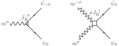
Figure 1: Interaction vertices

The first observation is easy to demonstrate. For small fluctuations about the ordered state, the longitudinal interaction is approximately $J_{K}^{z}\int(\bar{\psi}_{\uparrow}\psi_{\uparrow}-\bar{\psi}_{\downarrow}\psi_{\downarrow})(1-\frac{1}{2}m^{+}m^{-})$. where we have used the constraint $m^{z}=\sqrt{1-m^{+}m^{-}}$. The “1” comes from the magnetization in the $z$-direction, and leads to a Zeeman shift in the energy of the conduction electrons. The reference point for our theory should therefore have a quadratic action for the fermions of the form

$$\mathcal{S}_{c} = \int d^{d}xd\tau\;\bar{\psi}_{\sigma}(\vec{x},\tau)\left(\partial_{\tau}-\frac{\nabla^{2}}{2m}-\mu+\sigma\Delta\right)\psi_{\sigma}(\vec{x},\tau)$$

where $\Delta\sim J_{K}^{z}\langle m^{z}\rangle\sim J_{K}^{z}$. We need to write this in momentum space where it has the effect of defining a spin-dependent Fermi wavevector: $K_{F\sigma}\equiv\sqrt{2m_{e}(\mu+\sigma\Delta)}$. Expression (LABEL:eq:quadraticFermionPart) is unchanged except for the new definition of $K_{F\sigma}$. We need to build an effective low-energy theory around this fixed point, where there is a gap of size $2\Delta$ between the up-spin and down-spin bands. This form of the fermionic spectrum is essential to correctly capture the damping of magnons via the Kondo interaction. The interaction vertices are represented diagrammatically in figure 1, while the leading contributions to the self energies are shown in figure 2. The real and imaginary parts of the retarded functions can be calculated exactly. For example, the contribution from diagram $\Pi^{A}$ is

$$\text{Re}\Pi_{R}^{A}(\vec{q},\omega) = -\frac{mJ_{K}^{+}J_{K}^{-}}{q\pi}\Big{[}q$$

$$+K_{F\uparrow}\text{sgn}(\zeta_{-,\uparrow})\Theta(|\zeta_{-,\uparrow}|-1)\sqrt{\zeta_{-,\uparrow}^{2}-1}$$

$$+K_{F\downarrow}\text{sgn}(\zeta_{+,\downarrow})\Theta(|\zeta_{+,\downarrow}|-1)\sqrt{\zeta_{+,\downarrow}^{2}-1}\Big{]}$$

$$\text{Im}\Pi_{R}^{A}(\vec{q},\omega) = \frac{mJ_{K}^{+}J_{K}^{-}}{q\pi}\Big{[}-K_{F\uparrow}\Theta(1-|\zeta_{-,\uparrow}|)\sqrt{1-\zeta_{-,\uparrow}^{2}}$$ (11)

$$+K_{F\downarrow}\Theta(1-|\zeta_{+,\downarrow}|)\sqrt{1-\zeta_{+,\downarrow}^{2}}\Big{]}$$

where we have defined $\zeta_{\pm,\sigma}\equiv\frac{\omega-2\Delta}{v_{F\sigma}q}\pm\frac{q}{2K_{F\sigma}}$, and $\sigma\in\{+,-\}$. The region in $(\omega,q)$-space where the imaginary part is non-zero is depicted in the main paper. A similar exact expression is also available in $d=3$, but the approximate form is perhaps more useful. The bubble $\Pi_{R}^{A}$ in the regime $\Delta\ll\omega\ll v_{F}q\ll\mu=K_{F}^{2}/(2m_{e})$ is approximately:

$$\Pi_{R}^{A}(\vec{q},\omega) \approx J_{K}^{+}J_{K}^{-}\rho_{0}^{(d)}\left(1+i\gamma_{d}\frac{\omega}{v_{F}q}\right)$$ (12)

where $\gamma_{d}$ is a constant prefactor which depends on the spatial dimension, and $\rho_{0}^{(d)}=\sum_{\sigma}\rho_{0,\sigma}^{(d)}$ is the density of states at the Fermi level. In two and three dimensions, the explicit expressions are $\rho_{0,\sigma}^{(d=2)}=\frac{m}{2\pi}$ and $\rho_{0,\sigma}^{(d=3)}=\frac{m}{2\pi^{2}}K_{F\sigma}$. The $\omega/q$ form of the damping is common to a variety of systems; in this case it signifies Landau damping of the magnons with spin 1 excitations of the fermions.

Figure 2: Self Energies

To satisfy Goldstone’s theorem, it is necessary for all the pieces of $\Pi$ to cancel in such a way that the full bosonic propagator emerges in massless form. In the gauge-fermion problem, this is a consequence of gauge invariance Tsvelik_book_SI . In our case, the cancellation is somewhat more subtle. First, note that the diagrams $\Pi^{C}$ and $\Pi^{D}$ are explicitly $O(J_{K}^{2})$. Diagrams $\Pi^{A}$ and $\Pi^{B}$, however, are both linear in $J_{K}$. This is obvious for $\Pi^{B}$, whose calculation is trivial:

$$\text{Re}\Pi_{R}^{B}(\vec{q},\omega) = -J_{K}^{z}(n_{\uparrow}-n_{\downarrow})$$

$$\text{Im}\Pi_{R}^{B}(\vec{q},\omega) = 0$$ (13)

The sign difference comes from the fact that there is a four-leg vertex $J_{K}^{z}$ for each spin, but the sign of the coupling constant depends on $\sigma$. The reason why $\Pi^{A}$ is linear in $J_{K}$ instead of $O(J_{K}^{2})$ can be seen from a simple calculation at $(\vec{q}=0,\omega=0)$, which is non-singular due to the different spin indices. After performing the Matsubara sum,

$$\Pi^{A}_{R}(\vec{0},0) = 2J_{K}^{+}J_{K}^{-}\int\frac{d^{d}K}{(2\pi)^{d}}\frac{n(\xi_{K,\uparrow})-n(\xi_{K,\downarrow})}{\xi_{K,\downarrow}-\xi_{K,\uparrow}}$$ (14)

$$= 2J_{K}^{+}J_{K}^{-}\int\frac{d^{d}K}{(2\pi)^{d}}\frac{n(\xi_{K,\uparrow})-n(\xi_{K,\downarrow})}{2J_{K}^{z}}$$

$$= \frac{J_{K}^{+}J_{K}^{-}}{J_{K}^{z}}(n_{\uparrow}-n_{\downarrow})$$

Therefore, when the Kondo coupling is SU(2) symmetric the mass terms cancel and $\Pi^{A}+\Pi^{B}\approx J_{K}^{2}\gamma_{d}|\omega|/q$ and thus $\chi^{-1}(\vec{q},i\omega)=q^{2}+\gamma_{d}J_{K}^{2}\frac{|\omega|}{q}$, where as usual we have neglected the linear in $\omega$ term because it is less relevant in the RG sense. This special form of the bosonic propagator has emerged in a number of other applications, the most famous example being the gauge-fermion problem. We will comment on its consequence a little later.

With the inclusion of damping, the quadratic action now becomes:

$$\mathcal{S}_{m} = \int d\omega d^{d-1}q_{\perp}dq_{\parallel}\;m^{+}\left(q_{\perp}^{2}+b\frac{\omega}{q_{\perp}}\right)m^{-}$$ (15)

$$\mathcal{S}_{c} = \int d\epsilon d^{d-1}k_{\perp}dk_{\parallel}\;\bar{\psi}_{\sigma}\left(i\epsilon-v_{F}k_{\parallel}-a_{\sigma}k_{\perp}^{2}\right)\psi_{\sigma}$$ (16)

where $a_{\sigma}$ and $b$ are simply couplings that control the relative scaling between different components of the action. Their dimensions will be chosen to ensure the quadratic action is scale invariant. Significantly, in this $z_{b}=3$ theory the Berry phase no longer controls the dynamics, being instead overwhelmed by the damping term. Physically, this is because the magnetization of the local moment system is no longer conserved by itself once it can exchange spin flips with the conduction electrons.

The scaling analysis now needs to be redone.

$$\left[\epsilon\right] = 1$$

$$\left[k_{\parallel}\right] = 1$$

$$\left[k_{\perp}\right] = 1/z_{b}=1/3$$

$$\left[a\right] = 1-1/z_{b}=2/3$$

$$\left[b\right] = 0$$

$$\left[\psi\right] = -(3z_{b}+d-1)/(2z_{b})=-(8+d)/6$$

$$\left[m\right] = -(2z_{b}+d+1)/(2z_{b})=-(7+d)/6$$ (17)

Note that in principle $a_{\sigma}$ and $\psi_{\sigma}$ could scale differently for different spin projections, but because of the way they enter the action, we scale them identically. With these choices, all the terms in the quadratic action are scale invariant. The Kondo coupling terms,

$$\mathcal{S}_{K}^{\pm} = J_{K}^{\pm}\int d^{d-1}q_{\perp}dq_{\parallel}d\omega d^{d-1}k_{\perp}dk_{\parallel}d\varepsilon$$ (18)

$$\times\Big{[}\bar{\psi}_{k+q,\uparrow}\psi_{k,\downarrow}m^{-}_{q}+\bar{\psi}_{k+q,\downarrow}\psi_{k,\uparrow}m^{+}_{q}\Big{]}$$

$$\mathcal{S}_{K}^{z} = J_{K}^{z}\int d^{d-1}q_{1\perp}dq_{1\parallel}d\omega_{1}d^{d-1}q_{2\perp}dq_{2\parallel}d\omega_{2}d^{d-1}k_{\perp}dk_{\parallel}d\varepsilon\;$$

$$\qquad\times\Big{[}\bar{\psi}_{k+q_{1}-q_{2},\uparrow}\psi_{k,\uparrow}m^{+}_{q_{1}}m^{-}_{q_{2}}+\bar{\psi}_{k+q_{1}-q_{2},\downarrow}\psi_{k,\downarrow}m^{+}_{q_{1}}m^{-}_{q_{2}}\Big{]}$$

are easily analyzed:

$$[\mathcal{S}_{K}^{\pm}] = 0$$

$$= [J_{K}^{\pm}]+2[d^{d-1}k_{\perp}dk_{\parallel}d\varepsilon]+2[\psi]+[m]$$

$$= [J_{K}^{\pm}]+2\frac{d-1+2z_{b}}{z_{b}}-2\frac{3z_{b}+d-1}{2z_{b}}$$

$$-\frac{2z_{b}+d+1}{2z_{b}}$$

$$\implies[J_{K}^{\pm}] = (3-d)/(2z)$$ (20)

$$\left[\mathcal{S}_{K}^{z}\right] = 0$$

$$= [J_{K}^{z}]+3[d^{d-1}k_{\perp}dk_{\parallel}d\varepsilon]+2[\psi]+2[m]$$

$$= [J_{K}^{z}]+3\frac{d-1+2z_{b}}{z_{b}}-2\frac{3z_{b}+d-1}{2z_{b}}$$

$$-2\frac{2z_{b}+d+1}{2z_{b}}$$

$$\implies[J_{K}^{z}] = (1-d)/z$$ (21)

The inclusions of $\omega/q$ damping into the quadratic part of the boson action has the effect of changing the dynamics from $z_{b}=2$ to $z_{b}=3$, however, there is no change to the dimension of the spin-flip Kondo coupling. The longitudinal Kondo coupling is irrelevant for any $d>1$.

It turns out that a proper analysis of the fixed point requires insertion of the fermion self energy as well Altshuler94_SI , which we turn to next.

VI Electron Self Energy and Non-Fermi Liquid Behavior

In addition to the scaling analysis, we have another reason to determine the electron self-energy. Anticipating that the non-Fermi liquid contribution from the Kondo coupling to the magnons will be cut off at the energy of order $\omega\sim\omega_{c}\sim(I/W^{2})\Delta^{2}$, we wish to ascertain the magnitude of the non-Fermi liquid term at this cutoff scale. This will allow us to compare this term with some background Fermi liquid contributions. Since the Kondo coupling also occurs in the modified magnon propagator, we present here the calculation of the electron self-energy in some detail.

The leading order contribution to the electron self energy in $d=2$ is given by the dressed boson, bare fermion and no vertex correction, as depicted in figure 2.

$$\Sigma_{\bar{\sigma}}(\vec{K},i\epsilon) = J_{K}^{2}\int\frac{d^{2}qd\omega}{(2\pi)^{3}}G^{0}_{\sigma}(\vec{K}+\vec{q},i\epsilon_{m}+i\omega_{n})\chi(\vec{q},i\omega_{n})$$ (22)

$$= J_{K}^{2}\int\frac{d^{2}qd\omega}{(2\pi)^{3}}\frac{1}{i\epsilon+i\omega-\xi_{K+q,\sigma}}\;\frac{1}{q^{2}-\Pi(\vec{q},i\omega)}$$

$$= J_{K}^{2}\int\frac{d^{2}qd\omega}{(2\pi)^{3}}\frac{1}{i\epsilon+i\omega-\xi_{K\sigma}-\frac{Kq}{m}\cos\theta}$$

$$\times\frac{1}{q^{2}-\Pi(\vec{q},i\omega)}$$

From the previous section we have the result $\Pi(\vec{q},i\omega_{n})\approx-J_{K}^{2}\gamma\frac{|\omega|}{q}$. For the integral over $\theta$ we use: $\int_{0}^{2\pi}\frac{1}{z+i\cos\theta}=\frac{2\pi\text{sgn}\text{Re}(z)}{\sqrt{z^{2}+1}}$ for any complex $z$.

$$\Sigma_{\bar{\sigma}}(\vec{K},i\epsilon) = J_{K}^{2}\int\frac{qdqd\omega}{(2\pi)^{3}}\frac{1}{Kq/m}\frac{1}{q^{2}+J_{K}^{2}\gamma\frac{|\omega|}{q}}$$ (23)

$$\times\int d\theta\frac{1}{\frac{i\epsilon+i\omega-\xi_{K\sigma}}{\frac{Kq}{m}}-\cos\theta}$$

$$= -iJ_{K}^{2}\int\frac{qdqd\omega}{(2\pi)^{3}}\frac{1}{Kq/m}\frac{1}{q^{2}+J_{K}^{2}\gamma\frac{|\omega|}{q}}$$

$$\times\int d\theta\frac{1}{\frac{\epsilon+\omega+i\xi_{K\sigma}}{\frac{Kq}{m}}+i\cos\theta}$$

$$= -iJ_{K}^{2}\int\frac{qdqd\omega}{(2\pi)^{3}}\frac{1}{Kq/m}\frac{1}{q^{2}+J_{K}^{2}\gamma\frac{|\omega|}{q}}$$

$$\times\frac{2\pi\,\text{sgn}(\epsilon+\omega)}{\sqrt{\left(\frac{\epsilon+\omega+i\xi_{K\sigma}}{\frac{Kq}{m}}\right)^{2}+1}}$$

But in the regime of interest, and with the momentum restricted to $K\approx K_{F}$, we have $\frac{\epsilon+\omega+i\xi_{K\sigma}}{K_{F}/m}\ll 1$. The self-energy then simplifies to

$$\Sigma_{\bar{\sigma}}(K_{F},i\epsilon) \approx -iJ_{K}^{2}\int\frac{qdqd\omega}{(2\pi)^{3}}\frac{1}{K_{F}q/m}\frac{2\pi\,\text{sgn}(\epsilon+\omega)}{q^{2}+J_{K}^{2}\gamma\frac{|\omega|}{q}}$$

$$= -J_{K}^{2}\frac{im}{(2\pi)^{2}K_{F}}\int_{0}^{\Lambda}dq\int_{-\infty}^{\infty}d\omega\frac{\text{sgn}(\epsilon+\omega)}{q^{2}+J_{K}^{2}\gamma\frac{|\omega|}{q}}$$

This integral is a little tricky. First note that the frequency integral should have a cutoff, but this is complicated by the presence of the sgn function. It would be incorrect to simply shift variables $\omega\to\omega+\epsilon$. The essential identity we need is:

$$\int_{-\Lambda}^{\Lambda}d\omega f(\omega)\text{sgn}(\omega+\epsilon) = 2\int_{0}^{\epsilon}d\omega f(\omega)$$ (25)

which is only true for even functions: $f(\omega)=f(-\omega)$. To see where this comes from, note first that for even functions:

$$\int_{a}^{b}d\omega f(\omega) = -\int_{-a}^{-b}d\omega f(\omega)$$

Next, to handle the sgn function we partition the integral into four regions:

$$\int_{-\Lambda}^{\Lambda}d\omega f(\omega)\text{sgn}(\omega+\epsilon) = -\int_{-\Lambda}^{-\epsilon}d\omega f(\omega)+\int_{-\epsilon}^{0}d\omega f(\omega)$$

$$+\int_{0}^{\epsilon}d\omega f(\omega)+\int_{\epsilon}^{\Lambda}f(\omega)$$

where the minus sign is the result of the sgn function. Now we use the identity valid for even functions:

$$\int_{-\Lambda}^{\Lambda}d\omega f(\omega)\text{sgn}(\omega+\epsilon) = \int_{\Lambda}^{\epsilon}d\omega f(\omega)-\int_{\epsilon}^{0}d\omega f(\omega)$$

$$+\int_{0}^{\epsilon}d\omega f(\omega)+\int_{\epsilon}^{\Lambda}f(\omega)$$

$$= 2\int_{0}^{\epsilon}d\omega f(\omega)$$

Armed with this identity, the self energy is:

$$\Sigma_{\bar{\sigma}}(K_{F},i\epsilon) \approx -J_{K}^{2}\frac{2im}{(2\pi)^{2}K_{F}}\int_{0}^{\infty}dq\int_{0}^{\epsilon}d\omega\frac{1}{q^{2}+J_{K}^{2}\gamma\frac{|\omega|}{q}}$$ (26)

$$= -J_{K}^{2}\frac{2im}{(2\pi)^{2}K_{F}J_{K}^{2}\gamma}\int_{0}^{\infty}dqq\log\left(1+J_{K}^{2}\frac{\gamma\epsilon}{q^{3}}\right)$$

$$= -\frac{i2m}{(2\pi)^{2}K_{F}\gamma}\frac{\pi}{\sqrt{3}}\left(J_{K}^{2}\gamma\epsilon\right)^{2/3}$$

Had we used a cutoff on the q-integral, we would have ended up with some unsightly hypergeometric functions whose asymptotic form is the same as above, so it is easier to just set the cutoff to infinity straight away. For convenience, we have so far dropped the stiffness ($\rho_{s}$) factor in the $q^{2}$ term of the boson propagator. Reintroducing this factor, and taking $\rho_{s}\propto I$, we end up with the conduction electron self-energy quoted in the main text, Eq. (7).

Redoing the calculations for $d=3$ is relatively straightforward, although now the integral will be UV divergent. The only difference is that now we set $\vec{K}$ onto the x-axis since the $\phi$ variable is the one that runs from $0\to 2\pi$. This allows us to use the same identity on the $\phi$ integral that we used in the $d=2$ case for the $\theta$ integral.

$$\Sigma_{\bar{\sigma}}(\vec{K},i\epsilon) = J_{K}^{2}\int\frac{q^{2}dq\sin\theta d\theta d\omega}{(2\pi)^{4}}\frac{1}{Kq/m}\frac{1}{q^{2}+J_{K}^{2}\gamma\frac{|\omega|}{q}}$$

$$\times\int d\phi\frac{1}{\frac{i\epsilon+i\omega-\xi_{K\sigma}}{\frac{Kq}{m}}-\cos\phi}$$

$$= -iJ_{K}^{2}\int\frac{q^{2}dq\sin\theta d\theta d\omega}{(2\pi)^{4}}\frac{1}{Kq/m}\frac{1}{q^{2}+J_{K}^{2}\gamma\frac{|\omega|}{q}}$$

$$\times\int d\phi\frac{1}{\frac{\epsilon+\omega+i\xi_{K\sigma}}{\frac{Kq}{m}}+i\cos\phi}$$

$$= -iJ_{K}^{2}\int\frac{q^{2}dq\sin\theta d\theta d\omega}{(2\pi)^{4}}\frac{1}{Kq/m}\frac{1}{q^{2}+J_{K}^{2}\gamma\frac{|\omega|}{q}}$$

$$\times\frac{2\pi\,\text{sgn}(\epsilon+\omega)}{\sqrt{\left(\frac{\epsilon+\omega+i\xi_{K\sigma}}{\frac{Kq}{m}}\right)^{2}+1}}$$

Within the regime of interest this simplifies to

$$\Sigma_{\bar{\sigma}}(K_{F},i\epsilon) \approx -J_{K}^{2}\frac{2im}{(2\pi)^{3}K_{F}}\int qdq\int_{0}^{\epsilon}d\omega\frac{1}{q^{2}+J_{K}^{2}\gamma\frac{|\omega|}{q}}$$ (27)

$$= \frac{-2J_{K}^{2}im}{(2\pi)^{3}K_{F}J_{K}^{2}\gamma}\int_{0}^{\Lambda}dqq^{2}\log\left(1+\frac{J_{K}^{2}\gamma\epsilon}{q^{3}}\right)$$

$$= -\frac{2im}{(2\pi)^{3}K_{F}\gamma}\Bigg{[}\Lambda^{3}\log\left(1+\frac{J_{K}^{2}\gamma\epsilon}{\Lambda^{3}}\right)$$

$$+J_{K}^{2}\gamma\epsilon\log\left(1+\frac{\Lambda^{3}}{J_{K}^{2}\gamma\epsilon}\right)\Bigg{]}$$

$$\approx -\frac{2im}{(2\pi)^{3}K_{F}\gamma}\Bigg{[}J_{K}^{2}\gamma-J_{K}^{2}\gamma\log\epsilon$$

$$+J_{K}^{2}\gamma\log\frac{\Lambda^{3}}{J_{K}^{2}\gamma}\Bigg{]}\epsilon+O(\epsilon^{2})$$

So the leading singularity in $d=3$ is:

$$\Sigma \propto iJ_{K}^{2}\epsilon\log\epsilon$$ (28)

Again, recovering the stiffness factor leads to the form of the conduction electron self-energy presented in the main text, Eq. (7).

Holstein, Norton, and Pincus were the first to show that the transverse electromagnetic field coupling remains unscreened and can in principle lead to non-Fermi liquid behavior Holstein73_SI . For a real electromagnetic field, the smallness of the fine structure constant suppresses this effect to extremely low temperatures. Related non-Fermi liquid form appears in the gauge-fermion problem Lee89_SI ; Polchinski93_SI ; Altshuler94_SI . More recently, similar self energies have been found near quantum critical points and the nematic fermi fluid Rech06_SI ; Efremov08_SI ; Oganesyan01_SI . The prevalence of this self energy results from the generic presence of a massless $z_{b}=3$ boson coupled to a system with a Fermi surface. The problem we have considered here has some important formal differences from the gauge-fermion and critical Fermi liquid cases, even in the $z_{b}=3$ continuum regime. One difference is in the mechanism by which the boson propagators are gapless. In the gauge-fermion problem, gauge invariance guarantees the cancellation of the mass term upon adding the bubble and tadpole diagrams in a large-N calculation of the self energy of the vector potential Tsvelik_book_SI . At the ferromagnetic QCP, the divergence of the correlation length ($\xi^{-2}\to 0$) leads to gapless quantum critical fluctuations. In our case, it is the SU(2) spin symmetry of the Kondo interaction which dictates that the contribution from the longitudinal channel exactly cancels that from the transverse channel. A similar effect from the longitudinal mode of the ordered itinerant antiferromagnet was recently discussed by Vekhter04_SI , and we suspect that the cancellation argument we advance here may apply to their case as well. Another feature that is unique to our problem corresponds to the specific non-linear terms [Eq. 4] that occur here, which come into play in our RG analysis. We have shown that these terms, while relevant for the pure Heisenberg problem, become irrelevant when the Kondo coupling to the fermions is introduced.

We now turn to how the self-energy correction to fermions modify the damping term in the QNL$\sigma$M given in Eq. (12). The damping remains to have the $\omega/q$ form. For the regime of our interest here, $\omega\sim q^{3}$, both the self-energy and vertex corrections to the damping term are negligble. For generic $|\omega|\ll q$, the self-energy and vertex corrections cancel with each other leaving a subleading contribution Altshuler94_SI ; Kim94_SI .

We close this section by noting that, even though we are deep in the ferromagnetically ordered region, the phase space involved in the regime we are considering is similar to that of fermions coupled to $z=3$ ferromagnetic quantum critical fluctuations. Parallel to the calculations in the latter case, the temperature dependences of the electrical resistivity and specific heat have the non-Fermi liquid form given in the main text.

VII Scaling with fully dressed propagators

Now that we have the expression for the electron self energy we can finally incorporate it into the fixed point and redo the scaling analysis.

$$\mathcal{S}_{m} = \int d\omega d^{d-1}q_{\perp}dq_{\parallel}\;m^{+}\left(q_{\perp}^{2}+b\frac{\omega}{q_{\perp}}\right)m^{-}$$ (29)

$$\mathcal{S}_{c} = \int d\epsilon d^{d-1}k_{\perp}dk_{\parallel}\;\bar{\psi}_{\sigma}\left(|\epsilon|^{d/z_{b}}-v_{F}k_{\parallel}-a_{\sigma}k_{\perp}^{2}\right)\psi_{\sigma}$$

Note that the self energy correction to the fermion in $d=3$ is actually $\epsilon\log\epsilon$, but for the purposes of scaling we can simultaneously treat the cases $d=2$ and $d=3$ by analyzing the form $\epsilon^{d/z_{b}}$. To make every term in the quadratic action scale invariant we make the assignments:

$$\left[k_{\perp}\right] = 1/d$$

$$\left[k_{\parallel}\right] = 1$$

$$\left[\epsilon\right] = z_{b}/d=3/d$$

$$\left[a_{\sigma}\right] = 1-2/d$$

$$\left[\psi\right] = -(3d+z_{b}-1)/(2d)=-(3d+2)/(2d)$$

$$\left[m\right] = -(2d+z_{b}+1)/(2d)=-(2d+4)/(2d)$$ (31)

Inserting these dimensions into the Kondo coupling produces:

$$\left[J_{K}^{\pm}\right] = (3-z_{b})/(2d)=0$$ (32)

$$\left[J_{K}^{z}\right] = (3-z_{b}-d)/d=-1$$ (33)

In both $d=2$ and $d=3$, we find that the insertion of the self energies has led to the marginality of the transverse Kondo coupling, and the irrelevance of the longitudinal channel. This demonstrates that with the correct self energies built into the theory, which references the appropriate stable fixed point, there is never any unstable flow of the Kondo coupling. The ferromagnetic phase with a small Fermi surface is stable to the Kondo coupling.

Parenthetically, note that the magnon scattering term scales like:

$$\mathcal{S}_{m}^{(4)} \sim g\int\left(d^{d-1}q_{\perp}dq_{\parallel}d\omega\right)^{3}(q_{\perp}m)^{4}$$ (34)

$$\implies\left[g\right] = -\frac{3(d-1+d+z_{b})+4-2(2d+z_{b}+1)}{d}$$ (35)

$$= \frac{1-z_{b}-2d}{d}$$

$$= -2\frac{d+1}{d}$$

which is always irrelevant.

VIII The effect of the cutoff

Below the cutoff, $\omega<\omega_{c}\sim(I/W^{2})\Delta^{2}$ and $q<q_{c}\sim(K_{F}/W)\Delta$, the transverse Kondo coupling becomes irrelevant in the RG sense due to phase space restrictions. The longitudinal Kondo coupling, having the scaling dimension $(1-d)/z_{b}$, is irrelevant as well. The non-Fermi liquid effect will therefore be cut off in this range.

To ascertain the strength of the non-Fermi liquid contribution, we can compare the continuum contribution to the self energy, Eq. (7) of the main text, with the background Fermi liquid contribution at the cutoff frequency $\omega_{c}$. Adding a Coulomb interaction $u$ among the conduction electrons leads to a Fermi-liquid contribution to the self-energy of the order $\Sigma_{FL}(\epsilon)\sim u^{2}\rho_{0}^{3}\epsilon^{2}$. In $d=2$ we have

$$\Sigma_{NFL}(\epsilon\sim\omega_{c}) \sim (\rho_{0}J_{K}^{4}/I^{2})^{1/3}\omega_{c}^{2/3}\sim J_{K}^{8/3}/W^{5/3}$$

$$\Sigma_{FL}(\epsilon\sim\omega_{c}) = u^{2}\rho_{0}^{3}\omega_{c}^{2}\sim(u^{2}I^{2}/W^{7})J_{K}^{4}$$ (37)

In the parameter range we consider, $J_{K}\ll|I|\ll W$, $\Sigma_{NFL}(\epsilon\sim\omega_{c})$ is much larger than $\Sigma_{FL}(\epsilon\sim\omega_{c})$. Note that in three dimensions, $\Sigma_{NFL}(\epsilon\sim\omega_{c})\sim\rho_{0}J_{K}^{2}\omega_{c}/I\sim J_{K}^{4}/W^{3}$, leading to a similar conclusion.

IX Absence of Loop Corrections

IX.1 Vertex Corrections

For problems involving forward scattering of conduction electrons, the inability of vertex corrections to qualitatively modify leading order results has been established in related problems by a numbers of authors  Polchinski93_SI ; Altshuler94_SI ; Kim94_SI ; Yamamoto07_SI . The essence of the argument is a sort of Migdal’s theorem reminiscent of the suppression of vertex corrections in the electron-phonon problem AGD_SI . Previous work utilized a large number of fermion flavors, but we will take a slightly different approach which is more in line with the spirit of the fermionic RG and, like the original work by Migdal, focuses more explicitly on kinematics and phase space. The conclusions are essentially the same. The small parameter in our problem is $\Lambda/K_{F}\equiv 1/N_{\Lambda}$ which we use to define the large-$N_{\Lambda}$ expansion. (This $N_{\Lambda}\rightarrow\infty$ limit corresponds to asymptotically low energies, i.e., with the fermions approaching the Fermi surface.) Denoting the number of loops by $L$, the structure of the beta function is given by:

$$\beta(J_{K}) = b_{0}J_{K}+\frac{d}{d\log s}\sum_{L=1}^{\infty}\frac{b_{L}(s)}{N_{\Lambda}^{e(L,d)}}J_{K}^{2L+1}$$ (38)

$$\equiv b_{0}J_{K}+\frac{d}{d\log s}\Delta J_{K}$$

where loop integrals are performed over shells of width $\Lambda-\Lambda/s\approx\Lambda\log s$ with scaling parameter $s\equiv e^{\ell}\gtrapprox 1$. $L$ is equal to the number of integrations needed to compute the diagram. If the exponents $e(L,d)$ are positive for all values of $L$ and $d$ ($>1$), the beta function is given by the tree-level result ($b_{0}J_{K}$) in the large-$N_{\Lambda}$ limit, which means vertex corrections can be neglected. Since we have already shown that $b_{0}=0$, this would imply marginality to all orders. The goal of this section is to demonstrate that this is indeed the case.

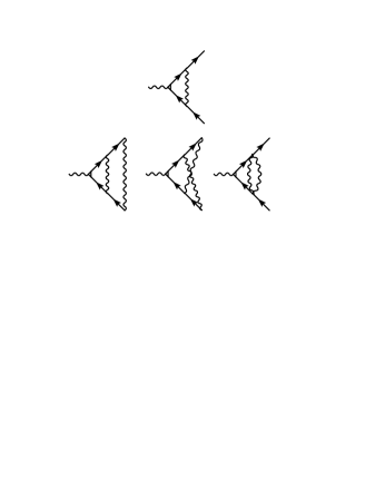
Figure 3: $L=1$ and $L=2$ vertex corrections. All propagators are dressed.

In what follows, we give two general arguments that demonstrate that vertex corrections become increasingly suppressed in the loop expansion. Specifically, a diagram with $L$-loops will come with a factor of $1/N_{\Lambda}^{L(d+3)/3}$, i.e. $e(L,d)=L(d+3)/3$. We also illustrate the principle by calculating an example $L=1$ diagram to demonstrate how this factor emerges. We work with cutoffs in units of $K_{F}$ so that $N_{\Lambda}\equiv 1/\Lambda$.

The first argument is essentially just power-counting. Every loop integral will introduce a factor of $\Lambda^{d+1}$ from the measure of integration. For $L$ loops, there will be $2L$ fermion propagators (see Fig 3) each carrying a factor of $\Lambda^{-d/z}$ with $z=3$. There will also be $L$ boson propagators which, because of the $\omega/q$ form of the boson self energy, scale like $O(1)$. Thus, each diagram with $L$-loops contributes the following amount of phase space.

$$\Delta J_{K} = \sum_{L=1}^{\infty}b_{L}(s)J_{K}^{2L+1}(\Lambda^{d+1})^{L}(\Lambda^{-d/z})^{2L}(\Lambda/\Lambda)^{L}$$ (39)

$$= \sum_{L=1}^{\infty}b_{L}(s)J_{K}^{2L+1}\Lambda^{[d(1-2/z)+1]L}$$

$$= \sum_{L=1}^{\infty}\frac{b_{L}(s)}{N_{\Lambda}^{(d+3)L/3}}J_{K}^{2L+1}$$

Therefore $e(L,d)=(d+3)L/3>0$, vertex corrects are kinematically suppressed, and the tree level result (marginality) is the entire story.

The careful reader will have noticed that other classes of diagrams are possible. For example, Fig 4a shows a self-energy insertion into the boson propagator. Iterates of diagrams like this might at first appear to compensate for some powers of $N_{\Lambda}$ due to the pure fermion loops. However, since we are using fully dressed propagators, this would be double counting. Such terms are already included by defining the fixed point action to have the $\omega/q$ self energy from the beginning.

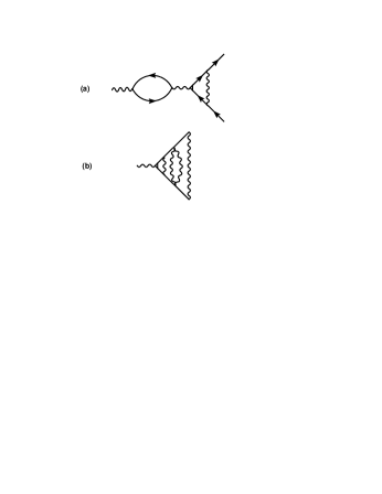
Figure 4: (a) Diagram which is not included because self energy corrections are already built into the dressed propagators. (b) An example of $L=4$ diagram with 6 fermion propagators and 4 boson propagators.

Another class of diagram is represented in Fig 4b, which is $L=4$ and with propagator powers of $G^{6}\chi^{4}=G^{2L-2}\chi^{L}$. More generally, an exhaustive classification of diagrams at order $L$, with $L$ even, will actually have $L/2+1$ subclasses which have factors

$$G^{2L}\chi^{L},G^{2L-2}\chi^{L},G^{2L-4}\chi^{L},\cdots,G^{L}\chi^{L}$$

If $L$ is odd, the series will terminate at $L+1$ rather than $L$, and there will be $(L+1)/2$ subclasses. However, since these subclasses only differ by smaller powers of $G$ than the $G^{2L}$ we considered above, it is easy to see that they will be subleading compared to the estimate given in equation 39.

The second way to obtain Migdal’s theorem more closely mirrors the antiferromagnetic case Yamamoto07_SI and the “leap to all loops” of the pure fermion problem Shankar94_SI . Begin by writing the quadratic parts of the action and rescaling all momenta and energies by $\Lambda$ so the limits of integration become dimensionless: $k\to\Lambda k$, $\epsilon\to\Lambda\epsilon$, etc.

$$\mathcal{S}_{c} = \Lambda^{d+1}\sum^{N_{\Lambda}}\int d^{d}kd\epsilon\;\psi^{\dagger}(i\epsilon^{d/z}\Lambda^{d/z}-\Lambda k_{\parallel}-\Lambda^{2}k_{\perp}^{2})\psi$$

$$\mathcal{S}_{m} = \Lambda^{d+1}\int d^{d}qd\omega\;m^{+}(\Lambda^{2}q^{2}+\omega/q)m^{-}$$ (41)

For simplicity, we have omitted some prefactors. To leading order in $1/N_{\Lambda}$ (small $\Lambda$), the dominant term in the fermionic part is $\epsilon^{d/z}$ ($\epsilon\log\epsilon$ in $d=3$), while the $\omega/q$ term is largest in the bosonic part. We therefore rescale fields according to these terms, obtaining:

$$\psi\to\Lambda^{-(4d/3+1)/2}\psi$$

$$m^{\pm}\to\Lambda^{-(d+1)/2}m^{\pm}$$ (42)

This allows us to estimate the phase space contribution of the interaction term. Rescaling according to this procedure, the Kondo coupling is given by:

$$J_{K}\int\Lambda^{2(d+1)}d^{d}kd\epsilon d^{d}qd\omega\Lambda^{-(4d/3+1)}\psi^{\dagger}\psi\Lambda^{-(d+1)/2}m^{\pm}$$

$$\propto J_{K}\Lambda^{(d+3)/6}$$ (43)

Associated with every power of $J_{K}$ is a factor $1/N_{\Lambda}^{(d+3)/6}$, and within the loop expansion the $L^{th}$-order correction is given by $\Delta J_{K}/J_{K}\propto J_{K}^{2L}\propto 1/N_{\Lambda}^{(d+3)/3}$, or $e(L,d)=(d+3)/3>0$, which is the same result we found earlier. Therefore vertex correction can be neglected and the tree-level result is asymptotically exact to all orders.

Note that the analog of this field rescaling for the pure fermion problem results in a four-fermion coupling given by $\Lambda u\int\psi^{4}$. In this case, Shankar found that the four-fermion coupling is still marginal despite the additional factor of $\Lambda$ induced by the field rescaling. We are simply to regard $\Lambda$ as a small parameter (in units of $K_{F}$), not a running variable. Within the momentum shell approach, the beta function is determined by finding the dependence on the parameter $s=e^{\ell}$ and computing the derivative $d/d\ell$, not by finding any explicit dependence on $\Lambda$ as is done in the field theory approach.

We have now proven that vertex corrections can be neglected in the large-$N_{\Lambda}$ limit. To demonstrate how the peculiar exponent $e(L,d)=(d+3)/3$ arises in a concrete example, let us calculate the first, $L=1$, vertex correction shown in figure 3.

$$\Delta J_{K}(\vec{p},i\epsilon;\vec{Q},i\Omega) = J_{K}^{3}\int d^{d}qd\omega G(\vec{p}+\vec{q},i\epsilon+i\omega)$$

$$\times G(\vec{p}+\vec{q}+\vec{Q},i\epsilon+i\omega+i\Omega)\chi(\vec{q},i\omega)$$

We can set the fermionic variables $\vec{p}=0$ (measured from the patch origin) and $\epsilon=0$ since any deviation would be irrelevant in the RG sense. In contrast, the variables $\vec{Q}$ and $\Omega$ belong to the external boson which we keep nonzero, keeping in mind that our problem has cutoffs $\omega_{c}$ and $q_{c}$.

$$\Delta J_{K}(0,0;\vec{Q},i\Omega) = J_{K}^{3}\int d^{d}qd\omega\frac{1}{i\epsilon_{0}^{1/3}|\omega|^{2/3}-v_{\uparrow}q_{\parallel}-v_{\uparrow}q_{\perp}^{2}/(2K_{F\uparrow})}\frac{\sqrt{q_{\perp}^{2}+q_{\parallel}^{2}}}{(q_{\perp}^{2}+q_{\parallel}^{2})^{3/2}+\gamma|\omega|}$$

$$\times\frac{1}{i\epsilon_{0}^{1/3}|\omega+\Omega|^{2/3}-v_{\downarrow}(q_{\parallel}+Q_{\parallel})-v_{\downarrow}(q_{\perp}^{2}+Q_{\perp}^{2})/(2K_{F\downarrow})}$$

One way to demonstrate Migdal’s theorem is to factorize integrands of momentum integrals according to a certain procedure, as detailed by several authors  Altshuler94_SI ; Abanov03_SI ; Chubukov05_SI . Physically, this relies of the fact that fermions are much faster than bosons. Formally, this can be accomplished by rescaling $v_{F}\to Nv_{F}$ and similarly for the coupling; see Appendix A of of ref Chubukov05_SI .

The validity of the factorization is not entirely obvious. Within a large-$N$ treatment, a thorough analysis has been done where numerical comparisons show that the factorization approximation only begins to break down at relatively high temperatures Abanov03_SI , outside the regime we consider here. In the next section, we show that the factorization of momentum integrations applies in the large-$N_{\Lambda}$ limit (without invoking large-$N$). For the rest of this section, we first proceed with such a factorization.

In such a case, the only parts of the integrand that depend on $q_{\perp}$ are the bosonic propagators. This allows us to define a momentum independent boson given by the fully momentum dependent propagator integrated along the Fermi surface:

$$\chi_{1}(i\omega;\Lambda_{\perp},q_{c}) \equiv \int d^{d-1}q_{\perp}\chi(\vec{q},i\omega)|_{q_{\parallel}=0}$$

$$= \int d^{d-1}q_{\perp}\frac{\Theta(q_{\perp}-q_{c\perp})\Theta(\Lambda_{\perp}-q_{\perp})}{q_{\perp}^{2}+\gamma\frac{|\omega|}{|q_{\perp}|}}$$

Note, once again, that we adopt the convention of ref. Altshuler94_SI in labeling parallel and perpendicular components. Also note that unlike other problems, we have a natural infrared regularization provided by the cutoff on bosonic modes. All integrals thus have both UV regularizations $\Lambda$ and IR regularizations $q_{c}$ and $\omega_{c}$. Moreover, loop integrals will be performed over momentum and energy shells, rather than extending the limits of integration to infinite intervals. This is the reason why we do not find a non-analytic $q^{3/2}$ correction to the static boson propagator, in contrast to theories for the itinerant ferromagnetic quantum critical point Chubukov04_SI .

To leading order in large-$N_{\Lambda}$, the vertex correction can now be written in factorized form:

$$\Delta J_{K}(0,0;Q_{\parallel},i\Omega) = J_{K}^{3}\int d\omega\chi_{1}(i\omega;\Lambda_{\perp},q_{c})$$

$$\times\int dq_{\parallel}\frac{1}{i\epsilon_{0}^{1/3}|\omega|^{2/3}-v_{\uparrow}q_{\parallel}}$$

$$\times\frac{1}{i\epsilon_{0}^{1/3}|\omega+\Omega|^{2/3}-v_{\downarrow}(q_{\parallel}+Q_{\parallel})}$$

Note that the dimensional dependence is confined to $\chi_{1}(i\omega)$, while the $q_{\parallel}$ dependence is isolated in the fermionic propagators. The dependence on external $Q_{\perp}$ has dropped out, which is higher order in $1/N_{\Lambda}$. To proceed, we consider $d=2$ for this illustrative example.

The range of integration requires some comment. Within the momentum-shell scheme, each loop integral consists of a number of “slabs” in phase space of width $\Lambda-\Lambda/s^{\eta}\approx\eta\Lambda\log s$, where $\eta$ is the scaling dimension of the appropriate direction. Within each slab, the integrand can be approximated by its value at the cutoff. For example, at one-loop we can write

$$I \equiv \int d\omega dq_{\parallel}dq_{\perp}f(\omega,q_{\parallel},q_{\perp})$$ (46)

$$\approx \left[q_{\perp}\right]\Lambda_{\perp}\log s\int d\omega dq_{\parallel}[f(\omega,q_{\parallel},\Lambda_{\perp})+f(\omega,q_{\parallel},-\Lambda_{\perp})]$$

$$+\left[q_{\parallel}\right]\Lambda_{\parallel}\log s\int d\omega dq_{\perp}[f(\omega,\Lambda_{\parallel},q_{\perp})+f(\omega,-\Lambda_{\parallel},q_{\perp})]$$

$$+\left[\omega\right]\Lambda_{\omega}\log s\int dq_{\parallel}dq_{\perp}[f(\Lambda_{\omega},q_{\parallel},q_{\perp})+f(-\Lambda_{\omega},q_{\parallel},q_{\perp})]$$

$$\equiv (\Lambda_{\perp}I_{\perp}+\Lambda_{\parallel}I_{\parallel}+\Lambda_{\omega}I_{\omega})\log s$$

We have divided the loop integral into a sum of $(d+1)$ terms which represent the slabs directed along each of the $(d+1)$ hyperplanes. This is simply the multidimensional generalization of the trivial result: $\int_{\Lambda/s^{\eta}}^{\Lambda}dx\;f(x)+\int^{-\Lambda/s^{\eta}}_{-\Lambda}dx\;f(x)\approx\eta\Lambda\log s[f(\Lambda)+f(-\Lambda)]$. Let us consider one of these slab integrals.

$$\Lambda_{\omega}I_{\omega} = \left[\omega\right]\Lambda_{\omega}J_{K}^{3}\int dq_{\perp}\frac{1}{q_{\perp}^{2}+\gamma\frac{\Lambda_{\omega}}{|q_{\perp}|}}\int dq_{\parallel}$$

$$\times\Big{[}\frac{1}{i\epsilon_{0}^{1/3}\Lambda_{\omega}^{2/3}-v_{\uparrow}q_{\parallel}}\frac{1}{i\epsilon_{0}^{1/3}(\Lambda_{\omega}+\omega_{c})^{2/3}-v_{\downarrow}(q_{\parallel}+q_{c})}$$

$$+\frac{1}{i\epsilon_{0}^{1/3}\Lambda_{\omega}^{2/3}+v_{\uparrow}q_{\parallel}}\frac{1}{i\epsilon_{0}^{1/3}(\Lambda_{\omega}-\omega_{c})^{2/3}+v_{\downarrow}(q_{\parallel}+q_{c})}\Big{]}$$

where we have take the external frequency and moment down to the cutoffs $q_{c}$ and $\omega_{c}$, and assumed $0<\omega_{c}<\Lambda_{\omega}$. This integral is factorized, with the first factor being given by

$$\chi_{1}(\omega=\Lambda_{\omega}) = \chi_{1}(\omega=-\Lambda_{\omega})$$ (48)

$$= \int dq_{\perp}\frac{1}{q_{\perp}^{2}+\gamma\frac{\Lambda_{\omega}}{|q_{\perp}|}}$$

$$= (1/3)(\gamma\Lambda_{\omega})^{-1/3}\Bigg{[}2\sqrt{3}\arctan\left(\frac{1-2q_{c}(\gamma\Lambda_{\omega})^{-1/3}}{\sqrt{3}}\right)-2\sqrt{3}\arctan\left(\frac{1-2q_{c}(\gamma\Lambda_{\omega})^{-1/3}}{\sqrt{3}}\right)$$

$$+2\log(q_{c}+(\gamma\Lambda_{\omega})^{1/3})-2\log(\Lambda_{\perp}+(\gamma\Lambda_{\omega})^{1/3})-\log(q_{c}^{2}-q_{c}(\gamma\Lambda_{\omega})^{1/3}+(\gamma\Lambda_{\omega})^{2/3})$$

$$+\log(\Lambda_{\perp}^{2}-\Lambda_{\perp}(\gamma\Lambda_{\omega})^{1/3}+(\gamma\Lambda_{\omega})^{2/3})\Bigg{]}$$

For an estimate of this factor, we must first take the limit $q_{c}\to 0$, since this must be smaller than the UV cutoffs:

$$\lim_{q_{c}\to 0}\chi_{1}(\omega=\Lambda_{\omega}) = (1/9)(\gamma\Lambda_{\omega})^{-1/3}\Bigg{[}\pi\sqrt{3}-6\sqrt{3}\arctan\left(\frac{1-2\Lambda_{\perp}(\gamma\Lambda_{\omega})^{-1/3}}{\sqrt{3}}\right)-6\log(\Lambda_{\perp}+(\gamma\Lambda_{\omega})^{1/3})$$ (49)

$$+3\log(\Lambda_{\perp}^{2}-\Lambda_{\perp}(\gamma\Lambda_{\omega})^{1/3}+(\gamma\Lambda_{\omega})^{2/3})\Bigg{]}$$

Next we set $\Lambda_{\omega}=\Lambda_{\perp}=\Lambda$, then take a small $\Lambda$ expansion, finding:

$$\chi_{1}\propto\Lambda/\gamma-\frac{2}{5\gamma^{2}}\Lambda^{3}+O(\Lambda^{5})$$ (50)

. The second factor is a more complicated integral.

$$\int(GG|_{\Lambda_{\omega}}+GG|_{-\Lambda_{\omega}}) = \int dq_{\parallel}\Big{[}\frac{1}{i\epsilon_{0}^{1/3}\Lambda_{\omega}^{2/3}-v_{\uparrow}q_{\parallel}}\frac{1}{i\epsilon_{0}^{1/3}(\Lambda_{\omega}+\omega_{c})^{2/3}-v_{\downarrow}(q_{\parallel}+q_{c})}$$ (51)

$$+\frac{1}{i\epsilon_{0}^{1/3}\Lambda_{\omega}^{2/3}+v_{\uparrow}q_{\parallel}}\frac{1}{i\epsilon_{0}^{1/3}(\Lambda_{\omega}-\omega_{c})^{2/3}+v_{\downarrow}(q_{\parallel}+q_{c})}\Big{]}$$

$$= \frac{1}{i\epsilon_{0}^{1/3}[(\Lambda_{\omega}+\omega_{c})^{2/3}-\Lambda_{\omega}^{2/3}]-v_{F}q_{c}}$$

$$\times\Bigg{\{}-\frac{2i}{v_{\uparrow}}\Big{[}\arctan\left(\frac{v_{\uparrow}\Lambda_{\parallel}}{\epsilon_{0}^{1/3}|\Lambda_{\omega}|^{2/3}}\right)-\arctan\left(\frac{v_{\uparrow}q_{c}}{\epsilon_{0}^{1/3}|\Lambda_{\omega}|^{2/3}}\right)\Big{]}$$

$$-\frac{1}{v_{\downarrow}}\Big{(}\frac{1}{2}\log\frac{\epsilon_{0}^{2/3}|\omega_{c}+\Lambda_{\omega}|^{4/3}+v_{\downarrow}^{2}(q_{c}-\Lambda_{\parallel})^{2}}{\epsilon_{0}^{2/3}|\omega_{c}+\Lambda_{\omega}|^{4/3}+v_{\downarrow}^{2}(q_{c}+\Lambda_{\parallel})^{2}}-\frac{1}{2}\log\frac{\epsilon_{0}^{2/3}|\omega_{c}+\Lambda_{\omega}|^{4/3}}{\epsilon_{0}^{2/3}|\omega_{c}+\Lambda_{\omega}|^{4/3}+4v_{\downarrow}^{2}q_{c}^{2}}$$

$$+i\arg[i\epsilon_{0}^{1/3}|\omega_{c}+\Lambda_{\omega}|^{2/3}-v_{\downarrow}(q_{c}-\Lambda_{\parallel})]-i\arg[i\epsilon_{0}^{1/3}|\omega_{c}+\Lambda_{\omega}|^{2/3}-v_{\downarrow}(q_{c}+\Lambda_{\parallel})]$$

$$+i\arg[i\epsilon_{0}^{1/3}|\omega_{c}+\Lambda_{\omega}|^{2/3}]-i\arg[i\epsilon_{0}^{1/3}|\omega_{c}+\Lambda_{\omega}|^{2/3}-2v_{\downarrow}q_{c}]\Big{)}\Bigg{\}}$$

$$+\frac{1}{i\epsilon_{0}^{1/3}[(\Lambda_{\omega}-\omega_{c})^{2/3}-\Lambda_{\omega}^{2/3}-v_{F}q_{c}]}$$

$$\times\Bigg{\{}-\frac{2i}{-v_{\uparrow}}\Big{[}\arctan\left(\frac{-v_{\uparrow}\Lambda_{\parallel}}{\epsilon_{0}^{1/3}|\Lambda_{\omega}|^{2/3}}\right)-\arctan\left(\frac{-v_{\uparrow}q_{c}}{\epsilon_{0}^{1/3}|\Lambda_{\omega}|^{2/3}}\right)\Big{]}$$

$$+\frac{1}{v_{\downarrow}}\Big{(}\frac{1}{2}\log\frac{\epsilon_{0}^{2/3}|-\omega_{c}+\Lambda_{\omega}|^{4/3}-v_{\downarrow}^{2}(q_{c}-\Lambda_{\parallel})^{2}}{\epsilon_{0}^{2/3}|-\omega_{c}+\Lambda_{\omega}|^{4/3}-v_{\downarrow}^{2}(q_{c}+\Lambda_{\parallel})^{2}}$$

$$-\frac{1}{2}\log\frac{\epsilon_{0}^{2/3}|-\omega_{c}+\Lambda_{\omega}|^{4/3}}{\epsilon_{0}^{2/3}|-\omega_{c}+\Lambda_{\omega}|^{4/3}-4v_{\downarrow}^{2}q_{c}^{2}}$$

$$+i\arg[i\epsilon_{0}^{1/3}|-\omega_{c}+\Lambda_{\omega}|^{2/3}+v_{\downarrow}(q_{c}-\Lambda_{\parallel})]$$

$$-i\arg[i\epsilon_{0}^{1/3}|-\omega_{c}+\Lambda_{\omega}|^{2/3}+v_{\downarrow}(q_{c}+\Lambda_{\parallel})]$$

$$+i\arg[i\epsilon_{0}^{1/3}|-\omega_{c}+\Lambda_{\omega}|^{2/3}]-i\arg[i\epsilon_{0}^{1/3}|-\omega_{c}+\Lambda_{\omega}|^{2/3}+2v_{\downarrow}q_{c}]\Big{)}\Bigg{\}}$$

where we have neglected terms of order $v_{\uparrow}-v_{\downarrow}\sim\Delta/\mu$, and used $\int dq_{\parallel}=\int dq_{\parallel}\Theta(q_{\parallel}-q_{c})\Theta(\Lambda_{\parallel}-q_{\parallel})$. Using the same procedure as for the previous factor, as well as the following simplifications, $q_{c}/\Lambda\ll 1$, $\omega_{c}/\Lambda\ll 1$, $\omega_{c}/q_{c}\ll 1$, and $\omega_{c}/\omega\ll 1$, we find the rather simple result:

$$\int(GG|_{\Lambda_{\omega}}+GG|_{-\Lambda_{\omega}}) \propto \Lambda^{1/3}\Lambda^{-2/3}=\Lambda^{-1/3}$$ (52)

Putting it all together, we find

$$\Lambda_{\omega}I_{\omega} \sim \left[\omega\right]\Lambda(\log s)\Lambda\Lambda^{-1/3}$$ (53)

$$= \frac{3}{2}\Lambda^{5/3}(\log s)$$

By a similar analysis, the other slab contributions can be shown to have the same exponent: $\Lambda_{\perp}I_{\perp}\sim\Lambda^{5/3}$ and $\Lambda_{\parallel}I_{\parallel}\sim\Lambda^{5/3}$. Therefore, the one-loop correction to the beta function is given by:

$$\delta J_{K} \sim \frac{d}{d\log s}\Lambda^{5/3}\log s$$ (54)

$$= \Lambda^{5/3}$$

$$= 1/N_{\Lambda}^{5/3}$$

which confirms our previous and more general derivations of Migdal’s theorem: $e(L=1,d=2)=(2+3)/3=5/3$.

To summarize, we have demonstrated Migdal’s theorem in three different ways, including an explicit calculation of the one-loop integral as a concrete example.

An interesting future direction would be to consider calculations of this sort with finite $\Lambda/K_{F}$, akin to $1/N_{\Lambda}$ corrections. In particular, it is easy to imagine that special bandstructures might possess Fermi surface features, such as nesting or van-Hove singularities, that might lead to significantly different conclusions. For such cases, however, it would then be necessary to consider specific materials with realistic bandstructures, and we would lose our ability to make universal statements. For this reason we remain content with the $N_{\Lambda}=\infty$ limit which should be valid under generic circumstances, and leave to future work detailed investigations of material-specific bandstructures where $1/N_{\Lambda}$ corrections might play an important role. We also point out that identifying the $N_{\Lambda}=\infty$ theory is in itself a non-trivial result. After all, Landau Fermi liquid theory is the $N_{\Lambda}=\infty$ limit of the interacting fermion problem Shankar94_SI which has been profoundly useful despite the fact that, by itself, $1/N_{\Lambda}$ corrections are not captured.

IX.2 Factorization of Momentum Integrals

The property of $q_{\parallel}-q_{\perp}$ integrations has previously been discussed within a large-$N$ limit, where $N$ is the number of fermion flavors Abanov03_SI . These theories typically perform loop integrations over all of phase space, in which case it becomes necessary to introduce the large factor $N$ in order to properly weight the desired kinematic range. Working with cutoffs explicitly, as we do, the integrals are more difficult to compute without the technology of residue calculus, however, the physical kinematic regime is more naturally apparent. Here, we demonstrate the validity of the factorization approximation used in the previous section, but we do not require a large number of fermion flavors. Instead, our large parameter is the ratio $N_{\Lambda}\equiv K_{F}/\Lambda$.

Consider a low-energy fermion represented by a point infinitesimally near the Fermi surface. This point on the Fermi surface defines the origin of our coordinate system. Since this patch of surface is defined by its normal, we decompose the coordinate system into components parallel and perpendicular to this normal vector. A low energy, forward scattering excitation involving this state will be contained within a box of size $\Lambda$ near this point of the Fermi surface, and we demand $\Lambda\ll K_{F}$. The momentum transfer between these two fermion states we label with $\vec{q}=(q_{\parallel},\vec{q}_{\perp})$. The factorization approximation is valid in the limit where the dimension of the box along the Fermi surface is much smaller than the Fermi wavevector: $\Lambda_{\perp}\ll K_{F}$. There are three ways to choose a small cutoff, as depicted in Fig 5. Either set $\Lambda_{\parallel}\ll\Lambda_{\perp}\sim K_{F}$, or $\Lambda_{\perp}\ll\Lambda_{\parallel}\sim K_{F}$, or $\Lambda_{\perp}\sim\Lambda_{\parallel}\ll K_{F}$. The first choice might lead one to believe that the number of patches is not large, which is not the case. The second option appears to suggest that $q_{\perp}\ll q_{\parallel}$, which is opposite to the regime we wish to consider. Furthermore, it includes high-energy excitations far from the mass shell. The third choice seems most natural, and it turns out to be the most convenient in terms of calculations as well, as indicated in the previous section. It might lead one to believe that the scaling is isotropic, but we will show below that this is not the case. Finally, a fourth possibility, where $\Lambda_{\perp}\sim\Lambda_{\parallel}\sim K_{F}$ has been used in calculations by other authors. When calculating with the fourth option, where loop integrals essentially extend to infinity, it is necessary to rescale the Fermi velocity by a large factor such as an artificially large number of fermion flavors Chubukov05_SI . The hope is that the $N=\infty$ results will be connected to the $N=2$ case we wish to understand, rather than the $N=0$ limit which is qualitatively different Sedrakyan09_SI ; Altshuler94_SI . We choose, instead, to rely on the fact that $\Lambda\ll K_{F}$ which does not require us to resort to large-$N$, but only large-$N_{\Lambda}$ which is simply the limit of the low-energy field theory.

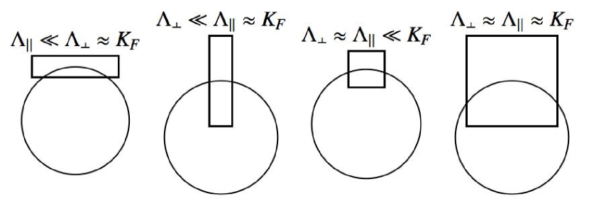
Figure 5: This figure depicts the various choices we have in choosing the size of our integration cutoffs in relation to each other, and the scale set by the Fermi momentum $K_{F}$. To restrict to low-energy excitations we must have $\Lambda_{\parallel}\ll K_{F}$. To ensure that we have a large number of patches, we must insist that $\Lambda_{\perp}\ll K_{F}$. The most convenient and sensible choice is to take $\Lambda_{\perp}\sim\Lambda_{\parallel}\ll K_{F}$. Even though the cutoffs are of similar size, we still have $q_{\perp}\gg q_{\parallel}$, as indicated by the next figure.

To see the small error made by the factorization approximation when $\Lambda_{\perp}\sim\Lambda_{\parallel}\ll K_{F}$, consider the one-loop vertex correction we calculated in the previous section, with and without the factorization approximation:

$$\Delta J_{K} = J_{K}^{3}\int d^{d}qd\omega\frac{1}{i\epsilon_{0}^{1/3}|\omega|^{2/3}-v_{\uparrow}q_{\parallel}-v_{\uparrow}q_{\perp}^{2}/(2K_{F\uparrow})}\frac{\sqrt{q_{\perp}^{2}+q_{\parallel}^{2}}}{(q_{\perp}^{2}+q_{\parallel}^{2})^{3/2}+\gamma|\omega|}$$ (55)

$$\times\frac{1}{i\epsilon_{0}^{1/3}|\omega+\Omega|^{2/3}-v_{\downarrow}(q_{\parallel}+Q_{\parallel})-v_{\downarrow}(q_{\perp}^{2}+Q_{\perp}^{2})/(2K_{F\downarrow})}$$

$$\Delta J_{K}\Big{|}_{\text{factorized}} = J_{K}^{3}\int d^{d}qd\omega\frac{1}{i\epsilon_{0}^{1/3}|\omega|^{2/3}-v_{\uparrow}q_{\parallel}}\frac{|q_{\perp}|}{q_{\perp}^{3}+\gamma|\omega|}\frac{1}{i\epsilon_{0}^{1/3}|\omega+\Omega|^{2/3}-v_{\downarrow}(q_{\parallel}+Q_{\parallel})}$$ (56)

The integrands are sharply peaked in phase space along surfaces defined by the zeros of the inverse propagators. For $\Delta J_{K}$ this corresponds to the surface defined by:

$$G^{-1}(q_{\perp},q_{\parallel},i\omega)G^{-1}(q_{\perp}+Q_{\perp},q_{\parallel}+Q_{\parallel},i\omega+i\Omega)$$

$$\times\chi^{-1}(q_{\perp},q_{\parallel},i\omega)=0$$ (57)

while for $\Delta J_{K}\big{|}_{\text{factorized}}$, the surface is defined by:

$$G^{-1}(0,q_{\parallel},i\omega)G^{-1}(0,q_{\parallel}+Q_{\parallel},i\omega+i\Omega)$$

$$\times\chi^{-1}(q_{\perp},0,i\omega)=0$$ (58)

The difference between these two cases is depicted in Fig. 6, where contours of constant energy are plotted in the momentum plane for $d=2$.

Figure 6: The left panel shows constant energy contours defined by the equation $G^{-1}(q_{\perp},q_{\parallel},i\omega)G^{-1}(q_{\perp}+Q_{\perp},q_{\parallel}+Q_{\parallel},i\omega+i\Omega)\chi^{-1}(q_{\perp},q_{\parallel},i\omega)=0$, corresponding to the peaked regions of the unfactorized (“exact”) integrand of the one-loop vertex correction with the unphysical value $\Lambda=K_{F}$. The middle panel is the same exact expression, but with the more reasonable $\Lambda=K_{F}/50$. Finally, the right panel depicts the constant energy contours of the highly peaked regions of the integrand using the factorization approximation; these curves are defined by: $G^{-1}(0,q_{\parallel},i\omega)G^{-1}(0,q_{\parallel}+Q_{\parallel},i\omega+i\Omega)\chi^{-1}(q_{\perp},0,i\omega)=0$. Clearly, the middle and right panels are very similar, justifying the use of the factorization approximation when $K_{F}$ is the largest scale.

Obviously, when $\Lambda\ll K_{F}$, the exact and factorized contours are almost indistinguishable. Only when $\Lambda\sim K_{F}$ does the curvature of the Fermi surface become apparent and the factorization approximation break down.

The figure also illustrates the fact that when $\Lambda\ll K_{F}$, the most highly peaked portions of the integrand occupy significant phase space where $q_{\perp}\gg q_{\parallel}$ for fixed energy (i.e. on each contour). This is so despite the fact that $\Lambda_{\perp}\sim\Lambda_{\parallel}$, and is the justification for the neglect of $q_{\parallel}$ terms in the bosonic propagators. At the same time, we neglect $q_{\perp}$ pieces of the fermionic propagators because $K_{F}$ is large.

A less graphical way to see the above is as follows. Because $\Lambda\ll K_{F}$, the $q_{\parallel}$ integration is dominated by the range ($\pm\Lambda^{2}/K_{F}$, $\pm\Lambda$). Over this range, the fermionic propagator can be approximated

$$G^{-1}(q_{\perp},q_{\parallel},i\omega) = \omega^{2/3}-v_{F}(q_{\parallel}+q_{\perp}^{2}/2K_{F})$$ (59)

$$\approx \omega^{2/3}-v_{F}q_{\parallel}.$$

The fermionic propagator tells us that the most important regions of the integrand are for $q_{\parallel}\sim\omega^{2/3}$. At the same time, the bosonic propagator is most highly peaked around $q\sim\omega^{1/3}$. This means that $q^{2}\sim\omega^{2/3}$. Since the pole of the fermion propagator will force $q_{\parallel}^{2}\sim\omega^{4/3}$, this means that the boson propagator must have $q_{\perp}^{2}\sim\omega^{2/3}\gg q_{\parallel}^{2}\sim\omega^{4/3}$, and thus

$$\chi^{-1}(q_{\perp},q_{\parallel},i\omega) \approx q_{\perp}^{2}+\gamma|\omega|/q_{\perp}$$ (60)

All these approximations become exact in the $N_{\Lambda}\rightarrow\infty$ limit. Eqs. (59,60) ensure the factorization of the $q_{\parallel}$ and $q_{\perp}$ integrations.

X Non-analytic corrections

An intriguing question for future studies is the effect of non-analytic Fermi-liquid corrections. Such non-analytic corrections to susceptibility and other physical properties already exist in a standard Fermi liquid theory Belitz_RMP_SI ; Efremov08_SI . In generic cases, such non-analytic corrections are relatively small. Empirically, it is in general hard to observe such non-analytic corrections. Even in the case of the quantum critical point of a weak ferromagnetic system, the existence of an extensive critical regime controlled by the fixed point without taking into account the non-analytic-Fermi-liquid corrections is supported by experimental observations Smith_Nature_SI . For the ferromagnetic phase of the Kondo lattice system we have considered, this effect is expected to be even smaller: due to the breakdown of the Kondo effect, the amplitudes of the non-analytic correction terms will be normalized in terms of the bare Fermi energy of the conduction electrons as opposed to a renormalized Kondo energy. More broadly, just like it is important to establish the Fermi liquid fixed point before such non-analytic corrections are analyzed in detail, we have focused on the existence of a small-Fermi-surface ferromagnetic fixed point.

References

- (1) Pandey, S. et al. Fermionic representation for the ferromagnetic Kondo lattice model: Diagrammatic study of spin-charge coupling effects on magnon excitations. Phys. Rev. B 77, 134447 (2008).
- (2) Kapetanakis, M. D. & Perakis, I. E. Magnetization relaxation and collective spin excitations in correlated double-exchange ferromagnets. Phys. Rev. B 78, 155110 (2008).
- (3) Read, N. & Sachdev, S. Continuum quantum ferromagnets at finite temperature and the quantum hall effect. Phys. Rev. Lett. 75, 3509-3512 (1995).
- (4) Wen. X. G. & Zee, A. Spin waves and topological terms in the mean-field theory of two-dimensional ferromagnets and antiferromagnets. Phys. Rev. Lett. 61, 1025-1028 (1988).
- (5) Yamamoto, S. J. & Si, Q. Fermi surface and antiferromagnetism in the Kondo lattice: an asymptotically exact solution in dimensions. Phys. Rev. Lett. 99, 016401 (2007).
- (6) Shankar, R. Renormalization-group approach to interacting fermions. Rev. Mod. Phys. 66, 129-192 (1994).
- (7) Altshuler, B. L., Ioffe, L. B. & Millis, A. J. Low energy properties of fermions with singular interactions. Phys. Rev. B 50, 14048-14065 (1994)
- (8) Yamamoto, S. J., & Si, Q. Renormalization group for mixed fermion-boson systems. Phys. Rev. B 81, 205106 (2010).
- (9) Sachdev, S. Quantum Phase Transitions (Cambridge University Press, Cambridge, 1999).
- (10) Tsvelik, A. Quantum Field Theory in Condensed Matter Physics (Cambridge University Press, Cambridge, 2003).
- (11) Holstein, T., Norton, R. E. & Pincus, P. de Haas-van Alphen effect and the specific heat of an electron gas. Phys. Rev. B 8, 2649-2656 (1973).
- (12) Lee, P. A. Gauge field, Aharonov-Bohm flux, and high-Tc superconductivity. Phys. Rev. Lett. 63, 680-683 (1989).
- (13) Polchinski, J. Low energy dynamics of the spinon-gauge system. Nucl. Phys. B 422, 617-633 (1994).
- (14) Rech, J., Pepin, C. & Chubukov, A. V. Quantum critical behavior in itinerant electron systems: Eliashberg theory and instability of a ferromagnetic quantum critical point. Phys. Rev. B 74, 195126 (2006).
- (15) Efremov, D. V., Betrouras, J. J. & Chubukov, A. V. Non-analytic behavior of 2D itinerant ferromagnet. arXiv:0804.2736v1.
- (16) Oganesyan, V., Fradkin, E. & Kivelson, S. A. Quantum theory of a nematic Fermi fluid. Phys. Rev. B 74, 195126 (2001).
- (17) Vekhter, I. & Chubukov, A. V. Non-Fermi-Liquid behavior in itinerant antiferromagnets. Phys. Rev. Lett. 93, 016405 (2004).
- (18) Kim, Y. B., Furusaki, A., Wen, X. G., & Lee, P. A. Gauge-invariant response functions of fermions coupled to a gauge field Phys. Rev. B 50, 17917 (1994).
- (19) Abrikosov, A. A., Gorkov, L. P. & Dzyaloshinski, I. E. Methods of Quantum Field Theory in Statistical Physics (Dover Publications, New York, 1975).
- (20) Abanov, A., Chubukov, A. V., & Schmalian, J. Quantum-critical theory of the spin-fermion model and its application to cuprates: normal state analysis. Adv. Phys. 52, 119 218 (2003).
- (21) Chubukov, A. V., & Schmalian, J. Superconductivity due to massless boson exchange in the strong-coupling limit. Phys. Rev. B 72, 174520 (2005).
- (22) Chubukov, A. V., Pepin, C., & Rech, J. Instability of the quantum critical point of itinerant ferromagnets Phys. Rev. Lett. 92, 147003 (2004).
- (23) Sedrakyan, T. A., & Chubukov, A. V. Fermionic propagators for 2D systems with singular interactions. Phys. Rev. B 79, 115129 (2009).
- (24) Belitz, D., Kirkpatrick, T. R., & Vojta, T. How generic scale invariance influences quantum and classical phase transitions. Rev. Mod. Phys. 77, 579-632 (2005).
- (25) Smith, R. P. et al. Marginal breakdown of the Fermi-liquid state on the border of metallic ferromagnetism. Nature 455, 1220-1223 (2008).