AzTEC Millimetre Survey of the COSMOS Field - II. Source Count Overdensity and Correlations with Large-Scale Structure

Abstract

We report an over-density of bright sub-millimetre galaxies (SMGs) in the 0.15 deg² AzTEC/COSMOS survey and a spatial correlation between the SMGs and the optical-IR galaxy density at $z\mathrel{\lower 2.5pt\vbox{\hbox{$<$}\hbox{$\sim$}}}$ 1.1. This portion of the COSMOS field shows a $\sim 3\sigma$ over-density of robust SMG detections when compared to a background, or “blank-field”, population model that is consistent with SMG surveys of fields with no extragalactic bias. The SMG over-density is most significant in the number of very bright detections (14 sources with measured fluxes $S_{1.1mm}>6$ mJy), which is entirely incompatible with sample variance within our adopted blank-field number densities and infers an over-density significance of $\gg 4\sigma$. We find that the over-density and spatial correlation to optical-IR galaxy density are most consistent with lensing of a background SMG population by foreground mass structures along the line of sight, rather than physical association of the SMGs with the $z\mathrel{\lower 2.5pt\vbox{\hbox{$<$}\hbox{$\sim$}}}$ 1.1 galaxies/clusters. The SMG positions are only weakly correlated with weak-lensing maps , suggesting that the dominant sources of correlation are individual galaxies and the more tenuous structures in the region and not the massive and compact clusters. These results highlight the important roles cosmic variance and large-scale structure can play in the study of SMGs.

1 Introduction

Foreground structure, cosmic variance, and source environment can affect the observer’s perception and interpretation of the source population being probed in a particular survey. For example, gravitational lensing by massive foreground clusters affects both the observed flux of sources and the areal coverage of the survey in the source plane. These aspects of gravitational lensing have been utilised to probe the very faint sub-millimetre galaxy (SMG) population below the confusion limit imposed by the high density of faint SMGs relative to the survey beam size (e.g. Smail et al., 1997; Chapman et al., 2002; Cowie et al., 2002; Smail et al., 2002; Knudsen et al., 2006; Wilson et al., 2008). The measured (sub)millimetre fluxes of sources found in the direction of very massive clusters can also be affected by, and confused with, the signal imposed through the Sunyaev-Zel’dovich effect on the cosmic microwave background (e.g. Wilson et al., 2008). Furthermore, surveys can be affected by foreground structures with high galaxy-densities, which increase the likelihood of galaxy-galaxy lensing by intervening galaxies and complicate counterpart identification at other wavelengths (Chapman et al., 2002; Dunlop et al., 2004).

Spectroscopic observations have shown that the vast majority of SMGs with detectable radio counterparts lie at an average redshift of $z\sim$ 2.2 (Chapman et al., 2005), while spectroscopic (Valiante et al., 2007) and photometric (e.g. Younger et al., 2007) analysis put many radio-faint SMGs at even higher redshifts. The average SMG is unlikely to be found at $z\mathrel{\lower 2.5pt\vbox{\hbox{$<$}\hbox{$\sim$}}}1$, however it remains to be seen if the $z\sim 1$ SMG population can be locally enhanced due to large-scale structure and cosmic variance. Some evidence exists for increased number densities of SMGs in mass-biased regions of the $z\mathrel{\lower 2.5pt\vbox{\hbox{$>$}\hbox{$\sim$}}}1$ Universe. Surveys towards several $z\sim 1$ clusters (Best, 2002; Webb et al., 2005) find a number density of SMGs in excess of the blank-field counts that can not be explained by gravitational lensing alone. This implies that some of the SMGs are physically associated with the clusters, although the number statistics are small and the lensing could be underestimated (Webb et al., 2005). Similar over-densities have been found towards high-redshift radio galaxies (Stevens et al., 2003; De Breuck et al., 2004; Greve et al., 2007) and $z>5$ quasars (Priddey et al., 2008), where lensing of background sources is less likely to be an issue. Spectroscopic observations have also found common redshifts amongst SMGs in the SSA22 and HDF fields, suggesting physical over-densities of SMGs at redshifts of 3.1 and 2.0, respectively (Chapman et al., 2005). Together, these surveys suggest that these massive dusty starbursts are prominent in moderate and high-redshift cluster/proto-cluster environments.

In this paper, we analyse the density and distribution of SMGs in the AzTEC/COSMOS survey (Scott et al., 2008). The AzTEC/COSMOS survey covers a region within the COSMOS field (Scoville et al., 2007) known to contain a high density of optical-IR galaxies and prominent large-scale structure at $z\mathrel{\lower 2.5pt\vbox{\hbox{$<$}\hbox{$\sim$}}}1.1$ (Scoville et al., 2007), including a massive $M\sim 10^{15}M_{\odot}$ cluster at $z\approx 0.73$ (Guzzo et al., 2007). In § 2 we present the 1.1 mm source counts for the AzTEC/COSMOS field, revealing a strong over-density of bright SMGs compared to the blank-field. We explore the nature of this over-density through examination of the spatial correlation between SMGs and the known large-scale structures (§ 3). Positive correlation between SMG positions and low-redshift large-scale structure has been previously detected statistically in 3 disjoint SCUBA surveys (Almaini et al., 2003, 2005). We now present a wide-field investigation of such correlations using the AzTEC/COSMOS survey, which has advantages in its contiguous size (0.15 deg²), broad range of low-redshift environments, and the availability of deep multiband imaging and reliable photometric redshifts (Ilbert et al., 2008).

This is the second paper describing the 1.1 mm results of the AzTEC/COSMOS survey. Paper I (Scott et al., 2008) presented the data-reduction algorithms, AzTEC/COSMOS map and source catalogue, and confirmation of robustness of the AzTEC/JCMT data and pointing. Additionally, seven of the brightest AzTEC/COSMOS sources have had high-resolution follow-up imaging at 890 $\micron$ using the Sub-Millimetre Array (SMA) and are discussed in detail in Younger et al. (2007). Spitzer IRAC colours of these SMGs, and others, are discussed in Yun et al. (2008).

2 Number counts in the COSMOS field

The number density of SMGs provides constraints on galaxy evolution models (e.g. Kaviani et al., 2003; Granato et al., 2004; Baugh et al., 2005; Negrello et al., 2007) and insights to the dust-obscured component of star formation in the high-redshift Universe. The number density also describes how these discrete objects contribute to the cosmic infrared background (CIB), as discussed in Paper I. In this paper, we focus on how the localised SMG number counts reflect large-scale structure. Before presenting the number counts for the AzTEC/COSMOS survey (§ 2.3 & § 2.5), we describe the technical details of the flux corrections (§ 2.1) and methods (§ 2.2) that are vital to the construction of unbiased source counts from typical SMG surveys. Here we expand on the flux correction techniques of Coppin et al. (2006) and provide new tests of these methods through simulation.

2.1 Flux Corrections

Surveys of source populations whose numbers decline with increasing flux result in blind detections that are biased systematically high in flux. This bias is typically referred to as “flux boosting” and results from the fact that detected sources have a higher probability of being an intrinsically dim source (numerous) coincident with a positive noise fluctuation than being a relatively bright source (scarce) coincident with negative noise. This effect is concisely described in Hogg & Turner (1998) and is extremely important for SMG surveys (see Figure 1) due to the relatively low $S/N$ of the measurements and a population that is known to decline steeply with increasing flux (e.g. Scott et al., 2006; Coppin et al., 2006, and references therein).

We calculate an intrinsic flux probability distribution for each potential AzTEC source using the Bayesian techniques outlined in Paper I and Coppin et al. (2005); Coppin et al. (2006). The probability of a source having intrinsic flux $S_{i}$ when discovered in a blind survey with measured flux $S_{m}\pm\sigma_{m}$ is approximated as

$$p(S_{i}|S_{m},\sigma_{m})={p(S_{i})p(S_{m},\sigma_{m}|S_{i})\over p(S_{m},\sigma_{m})}$$ (1)

where $p(S_{i})$ is the assumed prior distribution of flux densities, $p(S_{m},\sigma_{m}|S_{i})$ is the likelihood of observing $(S_{m},\sigma_{m})$ for a source of intrinsic flux $S_{i}$, and $p(S_{m},\sigma_{m})$ is a normalising constant. The resulting probability distribution is referred to as the posterior flux distribution, or PFD, throughout this section. We assume a Gaussian (normal) noise distribution for $p(S_{m},\sigma_{m}|S_{i})$ that is consistent with the noise in our map at the location of the discovered source. The prior, $p(S_{i})$, is generated from pixel histograms of 10,000 noiseless simulations of the astronomical sky – as would be seen in zero-mean AzTEC/JCMT maps – given our best estimate of the true underlying SMG population and distribution. For this paper, we assume the SMG population exhibits number count densities that are well described by a Schechter function (Schechter, 1976) of the form

$${dN\over dS}={N^{\ast}\over S^{\prime}}\left({S\over S^{\prime}}\right)^{\alpha+1}\mbox{exp}(-S/S^{\prime}).$$ (2)

This parametric form is a slight departure from that used in Paper I and in the SCUBA/SHADES survey (Coppin et al., 2006), with $N^{\ast}/S^{\prime}$ replacing the parameter $N^{\prime}$ found in Paper I. This form has the advantage of reducing the correlations between the normalising parameter and the parameters $S^{\prime}$ and $\alpha$. The normalising factor, $N^{\ast}$, is in units of deg^-2 and is independent of the observation wavelength when assuming the same source population and a constant flux ratio between the observing bands. For the Bayesian prior, we initially assume parameters of $[S^{\prime},N^{\ast},\alpha]=[1.34,5280,-2]$, which represent the best-fit Schechter function to the SCUBA/SHADES number counts (Coppin et al., 2006) when reparameterised to the form of Equation  2 and scaled to 1.1 mm assuming an 850 µm/1100 µm spectral index of 3.5 (flux ratio $\sim$ 2.5).

A second systematic flux bias in low-$S/N$ blind surveys results from source detections being defined as peak locations in the map. The measured source flux is, on average, biased high due to the possibility of large positive noise peaks lying nearby, but off-centre from, the true source position. This bias is minimised through point-source filtering and is sub-dominant to the flux boosting described previously. It is significant only for the lowest $S/N$ detections and is largely avoided by restricting our analysis to the most robust sources ($S/N\mathrel{\lower 2.5pt\vbox{\hbox{$>$}\hbox{$\sim$}}}4$). The remaining small bias ($b_{peak}<$ 0.2$\sigma_{m}$ for $S/N\geq 4$) is estimated through simulation and subtracted from the detected source flux ($S_{m}$) before calculating the PFD in Equation 1.

We validate these flux corrections through extensive simulation of the PFD. We generate 10,000 simulated maps by adding noiseless sky realisations to random noise maps using the prescription outlined in Paper I. Sources are randomly injected spatially (i.e. no clustering) and in accordance with the number counts prior assumed. We group recovered sources in the resulting maps according to their measured values ($S_{m},\sigma_{m}$), with each being mapped back to an intrinsic flux, $S_{i}$, defined as the maximum input flux found within $\sigma_{beam}=7.6^{\prime\prime}$ of the output source location. For each bin of measured values ($S_{m},\sigma_{m}$), the input $S_{i}$ values are binned and normalised to produce a simulated PFD.

Example simulation results are presented in Figure 1. Overall, the Bayesian approximation of the PFD (solid curve) provides a good estimate of the simulated probability distribution (histogram) at most fluxes. The differences at low flux and low $S/N$ are due to a combination of source confusion in the simulations, higher-order effects of the bias to peak locations, and other low level systematics. For the purposes of this paper, the Bayesian results are preferred to the simulated PFDs for their computational speed, resolution, and flexibility in priors. The strong differences between the simulated probability distributions (histograms) and the naive Gaussian distributions (dashed curves) demonstrate the significance of flux boosting in surveys of this type. It is important to note that flux boosting (as described above) is not related to the adopted detection threshold and that even the most robust detections can be significantly biased. For example, a source detected at $S/N=8$ in the AzTEC/COSMOS map will have been boosted by an average of 1.2 mJy ($\sim 1\sigma_{m}$), assuming the scaled SCUBA/SHADES SMG population.

Figure 1: Posterior Flux Distribution (PFD) for $S/N=4$ (left) and $S/N=5$ (right) detections in a map with noise $\sim 1.3$ mJy assuming an underlying source population consistent with the AzTEC/COSMOS results presented in § 2.3. The simulated probability distribution is shown as the histogram and is calculated as described in § 2.1. Error bars represent the 1$\sigma$ Poisson errors of the simulation results, limited only by the number of simulations computed. The Bayesian approximation is depicted as a solid curve. The dashed vertical line represents the measured flux, $S_{m}$. The dashed curve is the Gaussian probability distribution, $p(S_{m},\sigma_{m}|S_{i})$, which represents the distribution that might otherwise be assumed without flux boosting and/or false detection considerations.

2.2 Number Counts Derivation

The relative robustness of each source candidate is encoded in the PFD and is a function of both $S_{m}$ and $\sigma_{m}$, as opposed to merely $S_{m}$/$\sigma_{m}$, due to the population’s steep luminosity function. As in Paper I, we use the total probability of a source candidate being de-boosted to negative flux as the metric of relative source robustness. Coppin et al. (2006) found that $P(S_{i}\leq 0|S_{m},\sigma_{m})<0.05$ provided a natural threshold from which to select a large sample of robust SMGs without including a significant number of noise peaks, or “false detections”. This threshold also marks the point where the Bayesian approximation begins to suffer from low-level systematics, as suggested by the comparison of the Bayesian and simulated PFDs (Figure 1). Therefore, we will use this “null threshold” of 5% to define our catalogue of robust sources from which to estimate number counts. This threshold is equivalent to $S/N$ values of 4.1 - 4.3 for our range of $\sigma_{m}$ values, 1.2 - 1.4 mJy, assuming the scaled SCUBA/SHADES prior.

We derive the number counts from the catalogue of robust sources and their associated PFDs using a bootstrap sampling method similar to that used in Coppin et al. (2006). In each step of this method, the selected sources are randomly assigned fluxes according to their respective PFDs (Equation 1). These samples are binned by flux to produce differential ($dN/dS$) and integral ($N$($>S$)) source counts, with each bin being appropriately scaled for survey completeness and area. We introduce sample variance by sampling the robust source catalogue with replacement (e.g. Press et al., 1992), and by Poisson deviating the number of times the catalogue is sampled around the true number of detections. We repeat this process 20,000 times to determine uncertainty and correlation estimates for the number count bins.

Applying this sampling method to relatively small source catalogues results in a discretely sampled probability distribution for each number counts bin. This finite multinomial distribution can be non-Gaussian and asymmetric; therefore, we describe the uncertainty in the number counts as 68% confidence intervals that are approximated by linearly interpolating between the occupation numbers sampled in the bootstrap.

Survey completeness is estimated through simulation, in which sources of known intrinsic flux are randomly injected into noise map realisations one at a time and their output is tested against the null threshold source definition. Independent simulations confirm that this method provides excellent completeness estimations at all fluxes considered and that source confusion is not an issue given our beamsize (18”) and map depth ($\sigma>$ 1.1 mJy). Completeness is calculated as a function of intrinsic flux and averaged across the map to account for the slightly varying depth across the survey region considered. We calculate the effective completeness of each differential number counts bin by averaging the simulated completeness function within the bin, weighted by the assumed relative abundance of sources (i.e. the prior).

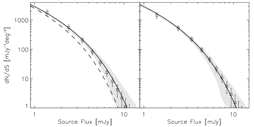
Figure 2: Simulated differential number count results (data points) using the extraction techniques described in § 2.2. The solid line represents the analytic source counts (Equation 2) used to populate the simulated maps, while the shaded region is the 1$\sigma$ dispersion incurred by randomly populating maps of this size (0.15 deg²). The left panel shows the results when assuming a prior based on the scaled SCUBA/SHADES results (dashed curve), while the right panel is for the “ideal” prior that matches the underlying input population (solid curve). Error bars represent the 1$\sigma$ dispersion from 1,000 simulations, while the errors in the means are typically smaller than the data symbols plotted.

We test these techniques by applying the same flux correction and number counts extraction algorithms to simulated maps with the same size and noise properties as those of the AzTEC/COSMOS survey. Figure 2 shows the extracted differential number counts from simulated maps using two different assumed priors. Both sets of simulated maps were populated with the same SMG population (solid line), which is similar to the final results of this AzTEC/COSMOS survey (§ 2.3). The right panel of Figure 2 shows the results of the ideal case where the Bayesian prior is the same distribution used to randomly populate the simulated maps, while the left panel shows the results when using the scaled SCUBA/SHADES prior (dashed curve), which differs from the simulated input population (solid curve). For both priors the extracted number counts are in excellent agreement with the injected population. The relatively small differences between the input and output counts in the ideal case are used as systematic correction factors in our final calculations. The lowest flux bin (1-2 mJy) suffers from very low (and poorly defined) completeness and is, in general, the most sensitive to the assumptions in the prior. For these reasons we will restrict our analysis in this paper to the number count results for fluxes $>2$ mJy, unless otherwise specified.

In Figure 2, the dispersion of the output source counts (error bars) is noticeably smaller than the dispersion of input source counts (shaded region) at high fluxes. This discrepancy reflects the correlation between output data points through our assumed prior. We characterise the overall bias to the assumed population by testing a wide range of priors against a static input population. For priors that are consistent with previous SMG surveys (e.g. Laurent et al., 2005; Coppin et al., 2006; Scott et al., 2006), the bias incurred is generally smaller than the formal 1$\sigma$ errors of the extracted counts in a survey of this size and depth. Larger biases can result for exceptionally poor priors (e.g. $>$ order of magnitude differences from the true population); however, in most cases the extracted number counts better represent the actual source population than the initial prior, making it possible to mitigate this bias through an iterative process that adjusts the prior based on the extracted counts. We apply this iterative method to the AzTEC/COSMOS number counts estimate in the next section.

2.3 AzTEC/COSMOS Number Counts

Figure 3: AzTEC/COSMOS integral source counts derived from the most robust AzTEC sources in the field using the techniques described in § 2.2. Filled circles (confidence bars omitted) represent the extracted counts using the initial assumed scaled SCUBA/SHADES prior (solid curve). Empty squares and 68% confidence bars represent the extracted counts after iteratively adjusting the prior to best represent the results of this survey. The dashed, dash-dotted, and dotted curves represent differential number counts fits to Eq. 2 with free parameters [$S^{\prime}$,$N^{\ast}$], [$S^{\prime}$], and [$N^{\ast}$], respectively. The horizontal dashed line represents the “survey limit”, defined here as the source density that will Poisson deviate to zero sources (per 0.15 deg²) 32.7% of the time. Open triangles and associated error bars represent the number counts found in the AzTEC GOODS-N survey (Perera et al., 2008) using the same techniques and have been shifted 4% to the left for clarity.

The AzTEC/COSMOS integrated number counts are shown in Figure 3. This field shows an excess of sources at all fluxes when compared to the scaled SCUBA/SHADES results (solid line). The number counts results are relatively insensitive to the choice of prior, with the initial analysis (filled circles) in agreement with those produced using an iterative prior (open squares). The “robust” source criterion of $P(S_{i}<0|S_{m},\sigma_{m})<0.05$ is somewhat more sensitive to the chosen prior, with the equivalent $S/N$ threshold in a $\sigma_{m}=1.3$ mJy region being 4.2 and 4.0 for the initial and final iterative priors, respectively. The final iterative prior deems a larger number of sources as robust compared to the initial prior due to the number of sources lying in this $S/N$ range. The corresponding effect on the survey completeness keeps this from being a runaway process, with the iterative number counts quickly converging within a few iterations.

The differential and integrated number counts of the AzTEC/COSMOS field are presented in Table 1. We fit the differential number counts to Equation 2 using Levenberg-Marquardt minimisation, incorporating the data covariance matrix to account for correlations between flux bins. Various fits to the data are presented in Table 2 and are shown in Figure 3. Given the size and depth of this survey, we constrain the parametric fits to flux bins between 2 and 10 mJy to avoid bins that are poorly sampled and prone to systematic errors. This range of flux values is relatively insensitive to the power-law parameter $\alpha$ (Equation  2); therefore, we fit the data while holding $\alpha$ constant at values of $-2$ and $-1$, which represent the SCUBA/SHADES result and a pure exponential, respectively. We also present similar fits to the SCUBA/SHADES number counts (Coppin et al., 2006) for comparison. The parametrised AzTEC/COSMOS results provide the maximum constraint on differential source counts at fluxes $\sim$ 4-5 mJy (depending on the parametrisation). For example, a two parameter ($S^{\prime}$,$N^{\ast}$; $\alpha$ fixed to $-2$) fit to Equation  2 constrains the AzTEC/COSMOS differential counts at 4.5 mJy to $84\pm 17$ deg^-2 mJy^-1.

Uncertainty in the flux calibration of the AzTEC/COSMOS survey is not included in these calculations and we believe it to be sub-dominant to the formal errors of the source flux, number counts, and fitted parameters. Calibration error estimates for individual observations during this observing season are 6-13% (Wilson et al., 2008). Any normally distributed random component of this error will be reduced in the final co-added map since this survey is composed of multiple observations spanning many nights/weeks and calibration measurements. Systematic error in the calibration is believed to be dominated by the 5% uncertainty in the flux density of our primary calibrator, Uranus (Griffin & Orton, 1993).

Flux Density	dN/dS	Flux Density	N($>$S)
(mJy)	(mJy-1deg-2)	(mJy)	(deg-2)
1.40	$1706.^{+666.}_{-1534.}$	1.0	$2610.^{+987.}_{-1346.}$
2.42	$535.^{+235.}_{-292.}$	2.0	$904.^{+232.}_{-319.}$
3.43	$204.^{+88.}_{-82.}$	3.0	$369.^{+85.}_{-103.}$
4.43	$84.^{+37.}_{-33.}$	4.0	$165.^{+37.}_{-48.}$
5.44	$38.^{+18.}_{-18.}$	5.0	$81.^{+22.}_{-27.}$
6.44	$19.^{+10.}_{-12.}$	6.0	$43.^{+15.}_{-19.}$
7.44	$11.^{+6.}_{-9.}$	7.0	$24.^{+11.}_{-15.}$
8.44	$6.5^{+4.2}_{-6.0}$	8.0	$13.^{+6.}_{-10.}$
9.44	$3.9^{+3.8}_{-3.6}$	9.0	$6.7^{+3.7}_{-6.7}$

Table 1: AzTEC/COSMOS differential and integral number counts using iterative adjustment of the prior. The differential number counts flux bins are 1 mJy wide and span interger flux values, with effective bin centres (first column) weighted according to the assumed prior. The lowest flux bin listed is particularly sensitive to uncertainties in the prior and such systematics are not included in the given 68% confidence intervals.

Data Set	$S^{\prime}$	$N^{\ast}$	$\alpha$	$\chi^{2}$
	(mJy)	(deg-2)
Az/COS	$1.83\pm 0.41$	$4420\pm 2720$	$-2$	0.21
Az/COS	$1.72\pm 0.12$	$5200$	$-2$	0.28
Az/COS	$1.36$	$9610\pm 1970$	$-2$	1.89
SHADES	$3.36\pm 0.49$	$5200\pm 1790$	$-2$	0.23
Az/COS	$1.31\pm 0.23$	$3570\pm 1790$	$-1$	0.59
SHADES	$2.39\pm 0.27$	$4370\pm 1170$	$-1$	0.21
MODEL1.1mm	$1.34$	$5280$	$-2$	$--$

Table 2: Fit results to the differential number counts and respective covariance matrix of the AzTEC/COSMOS ($1100~{}\micron$) and SCUBA/SHADES ($850~{}\micron$; Coppin et al., 2006) surveys. All fits are to the modified Schechter function given in Equation 2 while holding various parameters constant (those with no uncertainty given). To avoid strong systematics at low flux, all fits are limited to data with $S_{1100\micron}\geq 2$ mJy and $S_{850\micron}\geq 4$ mJy for the AzTEC and SCUBA surveys, respectively. The last row represents our assumed 1.1 mm blank-field model for the initial prior (scaled SCUBA/SHADES). $\chi^{2}$ values are unrealistically low, likely due to a combination of: (a) our uncertainties being assumed as Gaussian in the fit; and (b) additional correlation not accounted for in the linear Pearson covariance matrix constructed through the bootstrap sampling method (§ 2.2). These effects are also seen in the SCUBA/SHADES implementation of this algorithm (Coppin et al., 2006).

2.4 Blank-Field Model

It is immediately apparent that the AzTEC/COSMOS field is rich in bright sources when compared to other 1.1 mm surveys (see § 2.5). In order to quantify the significance of this potential over-density, we must first adopt an accurate characterisation of the true background (“blank-field”) population. The tightest published constraint on the SMG population is provided by the 850 $\micron$ SCUBA/SHADES survey (Coppin et al., 2006), which we convert to 1100 $\micron$ assuming an $850~{}\micron$/$1100~{}\micron$ power-law spectral index of $3.5$. This scaling is roughly consistent with the integrated number counts of the 1.1 mm Bolocam Lockman Hole survey (Laurent et al., 2005), which partially overlaps with the SCUBA/SHADES survey. Assuming the SCUBA and AzTEC observations are in the Rayleigh-Jeans regime of optically-thin thermal dust emission from the SMGs, our scaling is consistent with the sub-mm spectral indexes of bright IR galaxies in the local universe (Dunne et al., 2000; Dunne & Eales, 2001).

Using a scaled version of the number counts measured at a different observation wavelength carries the inherent risk that the two bands are sensitive to significantly different (although overlapping) source populations, as evidenced by the possible existence of sub-millimetre drop-outs (SDOs, Greve et al., 2008). The SCUBA 850 $\micron$ surveys would be relatively insensitive to these proposed SDOs due to a combination of high redshift ($z\gg 3$) and/or unusual spectral energy distributions (e.g. $T_{dust}\sim 10$ K). Therefore, it is important to verify the blank-field model with a direct measurement of 1.1 mm population.

The most robust characterisation of the AzTEC/COSMOS over-density comes through comparison to similar analyses of other AzTEC 1.1 mm surveys, which eliminates systematics between different instruments and minimises those related to calibration. The best AzTEC 1.1 mm blank-field constraints are being provided by the AzTEC 0.5 deg² survey of the SHADES fields. Initial results of the AzTEC/SHADES survey (using nearly identical algorithms as those applied to AzTEC/COSMOS) are consistent with our scaling of the SCUBA/SHADES counts. Our number counts model falls in the higher regions of the AzTEC/SHADES uncertainty interval (modelled differential counts are roughly $+$0.5$\sigma$ to $+$2.0$\sigma$ above the average AzTEC/SHADES counts in the flux range explored here) and is within the field-to-field variations measured in those large surveys; therefore, we believe our model represents a conservatively high estimate of the blank-field counts that is appropriate for robust qualification of the potential over-density.

We note that the AzTEC survey of the GOODS-N field (Perera et al., 2008) finds an SMG number density that is somewhat higher than our blank-field model; however, our model is within the $\sim 1\sigma$ uncertainty of that survey’s integrated number counts (Figure 3; note that the data points are correlated). The AzTEC/GOODS-N results imply an $S^{\prime}$ parameter ($S^{\prime}=1.25\pm 0.39$ mJy) that is consistent with our general scaling of the SCUBA/SHADES counts, but suggest systematically higher number counts (i.e. larger $N^{\ast}$ parameter). The small size of the GOODS-N survey (0.068 deg²) makes it highly susceptible to cosmic variance and clustering, thus reducing it’s viability as a measurement of the average sky. It also does not significantly constrain the bright ($S>$ 5 mJy) 1.1 mm source counts where the AzTEC/COSMOS over-density is most apparent (§ 2.5). The SCUBA survey of GOODS-N (Borys et al., 2003) already suggests the field may be overly rich in sub-millimetre sources, with number counts systematically higher than seen in the SCUBA/SHADES blank-field (Coppin et al., 2006), although the analyses of these two SCUBA surveys differ significantly and the difference in number counts could be partially systematic.

2.5 SMG Over-density

The source catalogue presented in Paper I suggests that the AzTEC/COSMOS field has a significantly larger number of bright 1.1 mm sources than might otherwise be expected for a survey of this size and depth. The density of sources in the AzTEC/COSMOS field with raw measured fluxes $\geq 6$ mJy is 3 times higher (14 sources in 0.15 sq. deg. field) than in the 1.1 mm Bolocam Lockman Hole survey of similar depth (3 sources in 0.09 sq. deg.; Laurent et al., 2005). The seven brightest AzTEC sources in the COSMOS field have been imaged using the Submillimeter Array (SMA) at 890 $\micron$, and they are shown to be single, unresolved sources at 2 arcsec resolution (Younger et al., 2007).

We compare the AzTEC/COSMOS number counts to the blank-field model discussed in § 2.4. Figure 3 shows that the AzTEC/COSMOS integrated source count estimates are clearly in excess of the scaled SCUBA/SHADES counts.

To estimate the probability of this excess happening by chance, we compare the number of robust sources detected in the AzTEC/COSMOS survey to the number recovered in simulated maps. In Figure 4 we show the distribution of the number of recovered sources in 10,000 simulations, each populated with a random realisation of the scaled SCUBA/SHADES counts. On average, 12.1 sources are recovered from each of the simulated maps, which is in agreement with the semi-analytical expectation value of 11.2 (calculated from the scaled SCUBA/SHADES results and simulated completeness of this survey) and the expected number of false detections ($\langle N_{false}\rangle\approx 1.2$). Application of the same source criteria (5% null threshold, scaled SCUBA/SHADES prior) to the real map results in 23 robust sources (32 if using the iterative prior), which is greater than in 99.7% of the simulations. The AzTEC/COSMOS source over-density is even more significant in the number of very bright sources, with 11 detected at $S/N~{}\geq$ 5 ($S_{m}~{}\mathrel{\lower 2.5pt\vbox{\hbox{$>$}\hbox{$\sim$}}}$ 6.2 mJy). Ten-thousand simulations of the blank-field model could produce no more than 6 such detections in a single map, thus inferring a $\gg 4\sigma$ significance in the number of bright sources.

Assuming the scaling of the SCUBA/SHADES counts accurately represents the blank-field SMG population at 1.1 mm, the parametric fits shown in Table 2 favour the over-density being described as a shift in the flux parameter $S^{\prime}$ over an increase in the normalisation parameter $N^{\ast}$. This is consistent with an apparent over-density caused by uniform amplification of the source fluxes. However, this solution is degenerate with an alternative scaling of the SCUBA/SHADES results – scaling with a flatter spectral index of $\sim 2.6$ also produces a good fit to the AzTEC/COSMOS number counts (dash-dotted curve of Figure 3). Therefore, an accurate representation of the blank-field population (§ 2.4) is critical to properly quantifying the over-density.

Figure 4: Distribution of the number of robust sources detected in 10,000 simulations (using 300 unique noise realisations) of the AzTEC/COSMOS observations when randomly populating the astronomical sky with the scaled SCUBA/SHADES number counts (solid histogram). Using the same source criteria, there are 23 robust sources detected in the AzTEC/COSMOS map (dashed vertical), which is greater than 99.7% of the simulations. A Gaussian fit to the simulation results (thin solid curve) shows 23 sources to be a 3.3$\sigma$ outlier. The difference between the simulation mean (solid vertical) and the semi-analytic expectation value (dotted vertical) reflects the number of false detections (i.e. $\sim$ 1 per map) for the scaled SCUBA/SHADES prior and chosen source threshold.

If taken alone, the over-density of SMGs in the AzTEC/COSMOS field would likely be explained away as simple cosmic variance in the SMG population as traced in a 0.15 deg² field. However, in the following sections we demonstrate that the over-density is due, in part, to foreground structure in the COSMOS field. Only with the rich multi-wavelength coverage of the COSMOS field and the relatively large size of the AzTEC map is this analysis possible.

3 Correlation Between AzTEC sources and Large Scale Structure in the COSMOS field

Having shown that the AzTEC/COSMOS field exhibits a significant excess of bright SMGs with respect to our adopted blank-field model, we explore the possibility that this over-density is due, in part, to a correlation of AzTEC sources with the prominent large-scale structures at $z\mathrel{\lower 2.5pt\vbox{\hbox{$<$}\hbox{$\sim$}}}1.1$ identified in this portion of the COSMOS field (Scoville et al., 2007). All correlation tests in this section are limited to the inner 0.15 deg² region of the AzTEC map where the uniformity in coverage simplifies the analysis.

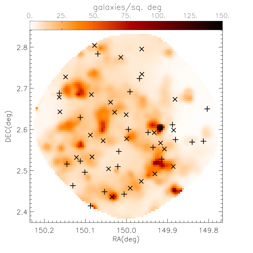
Figure 5: Smoothed surface density map of galaxies derived from the optical-IR catalogue of COSMOS galaxies (Scoville et al., 2007) in the 0.15 sq. deg area surveyed by AzTEC, where darker colours indicate more densely populated areas of the sky. The cross and plus symbols represent AzTEC sources detected at signal-to-noise ratios $S/N\geq 4$ and $4>S/N\geq 3.5$ (Scott et al., 2008), respectively.

The smoothed galaxy density map produced by the COSMOS consortium (Scoville et al., 2007, see Figure 5) shows a collection of dense regions in the the AzTEC covered area. We first look for coincidence with AzTEC sources by cross-correlating the surface-density of optical-IR galaxies in this map with the AzTEC source positions using a bi-dimensional Kolmogorov-Smirnov (K-S) test of similarity (Peacock, 1983; Fasano & Franceschini, 1987). Restricting this analysis to the 30 robust AzTEC sources detected at a $S/N\geq 4$, which have an estimated false detection rate of less than 7% (Scott et al., 2008), we find that the test cannot reject the null hypothesis that the distribution of AzTEC-source positions follows the surface density distribution of optical-IR galaxies. The test concludes that the difference between the SMG and optical-IR populations is smaller than 93.7% of the differences expected at random due to sample variance, often referred to as rejecting the null hypothesis at the 6.3% level, thus suggesting the distributions could indeed be similar.

The significance of the SMG positional correlation with the large-scale structure is further quantified by comparing the K-S $D$-statistic of the SMG catalogue to that of a homogeneous random distribution of the same number of sources, under the null hypothesis that they follow the surface density of optical-IR galaxies. This test determines that the AzTEC/COSMOS source distribution follows the optical-IR distribution more strongly than 98.9% ($\sim$ 2.5$\sigma$) of the random-position catalogues. The result is somewhat less significant, 91.1%, if we expand the comparison to the full $S/N\geq 3.5$ AzTEC/COSMOS catalogue, which is likely due to the increased number of false detections (from $\sim$ 1 to $\sim$ 11) at this lower $S/N$ threshold. These false detections (noise peaks) are inherently random and homogeneous in their distribution and dilute the correlation signal.

It is possible that only a fraction of the AzTEC source positions are correlated with the prominent large-scale structures detected in the COSMOS galaxy density map while a subset of randomly distributed source positions dilutes the sensitivity of the quadrant-based bi-dimensional K-S statistic discussed above. Therefore, we further test the hypothesised correlation by comparing the surface density of optical-IR galaxies within a small area surrounding AzTEC positions to that surrounding random positions in the map. Figure 6 shows the distribution of the galaxy densities at $z\mathrel{\lower 2.5pt\vbox{\hbox{$<$}\hbox{$\sim$}}}1.1$ projected within 30” (1.7 pixels in the smooth galaxy density map) of the AzTEC source positions, compared to the galaxy densities found around random positions within the AzTEC survey region. The two distributions are clearly different, with a one-dimensional K-S test rejecting the null hypothesis of identity at $>$ 99.99% and 97.2% levels for the $S/N\geq 4$ and $S/N\geq 3.5$ catalogues, respectively. The mean number of nearby optical-IR galaxies at $S/N\geq 4$ ($S/N\geq 3.5$) AzTEC source positions is larger than that at random positions in the map at a significance of 99.99% (99.5%) according to the non-parametric Mann-Whitney (MW) $U$-test.

Figure 6: Histogram of the galaxy density at $z\mathrel{\lower 2.5pt\vbox{\hbox{$<$}\hbox{$\sim$}}}1.1$ found within 30 arcsec of (a) AzTEC/COSMOS source candidates detected at $S/N\geq 3.5$ (dashed line) and (b) random positions in the AzTEC mapped area of COSMOS (solid line). The two populations are different at the 97.2% confidence level, using a one-dimensional K-S test. The galaxy densities are normalised to the mean galaxy density in the full AzTEC-covered area.

We can search in redshift space for the structures that contribute the most to the coincidence between AzTEC sources and the galaxy density in their “line of sight” using the photometric redshifts of the optical-IR population (Ilbert et al., 2008), which have a mean accuracy of $|\Delta z|/(1+z)\approx$ 0.01-0.02. Figure 7 shows a bar-representation of the MW probabilities that the mean integrated galaxy density around AzTEC sources is significantly larger than that around random positions in the map for various redshift slices. There is positive signal ($\mathrel{\lower 2.5pt\vbox{\hbox{$>$}\hbox{$\sim$}}}2\sigma$) arising at different redshift slices, most notably at $z\sim 0.65$. At redshifts $z>1.1$, the number of galaxies detected at optical-IR wavelengths decreases significantly, and the level of correlation found with AzTEC sources is well below the 2$\sigma$ threshold.

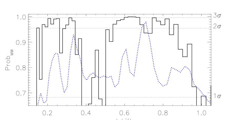
Figure 7: Bar-representation of the Mann-Whitney probability that the mean galaxy density around AzTEC sources at a given redshift slice is significantly larger than the mean galaxy density around random positions. Horizontal dotted lines represent the $1\sigma$, $2\sigma$, and $3\sigma$ significance levels, respectively. The blue-dotted curve shows the relative number of optical/IR galaxies contained within each redshift slice within the AzTEC covered area ($N_{\rm gal}(z)/N_{\rm total}*10.+0.60$).

The most prominent contribution to the AzTEC-optical/IR correlation lies at $0.6\mathrel{\lower 2.5pt\vbox{\hbox{$<$}\hbox{$\sim$}}}z\mathrel{\lower 2.5pt\vbox{\hbox{$<$}\hbox{$\sim$}}}0.67$, with the redshift slices within this range having MW probabilities of difference up to 99.98%. The smoothed galaxy density map for this redshift range is shown in Figure 8. Two prominent large-scale structures have been identified (Structures #1 and #24 in Scoville et al., 2007) within this redshift slice. Structure #1 at $z=0.73\pm 0.27$ has $1767$ optical-IR galaxy members and approximately spans (FWHM) $\Delta$ RA $=0.22$ deg and $\Delta$ Dec $=0.17$ deg. Structure #24, a less massive but very compact system that is X-ray detected, has 85 galaxy members and is at z $\sim$ 0.61. Structure #24, however, does not appear to contribute to the correlation, as no AzTEC sources fall within its primary extension. Structure #1 contains a rich core and represents a massive cluster ($\sim 10^{15}M_{\odot}$) at $z\approx 0.73$, which is clearly seen in the COSMOS weak-lensing convergence map (Massey et al., 2007) and in X-ray emission (Guzzo et al., 2007). This cluster lies outside the redshift span of strong correlation, but the filamentary structure that leads to it is part of the redshift slice under analysis (see Figure 8).

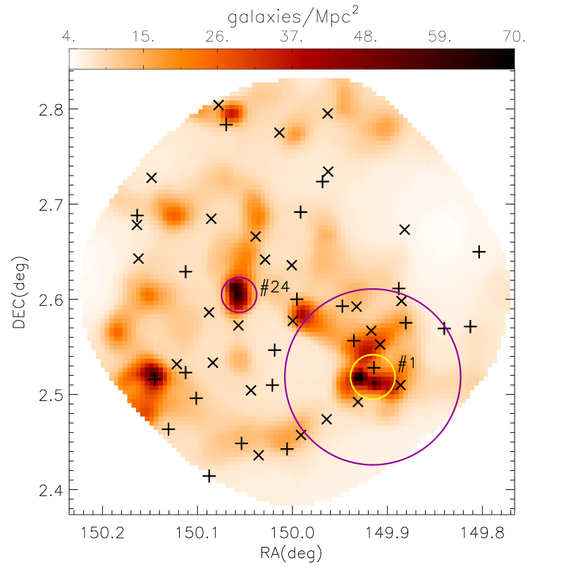
Figure 8: Smoothed surface density map of galaxies at $0.60\mathrel{\lower 2.5pt\vbox{\hbox{$<$}\hbox{$\sim$}}}z\mathrel{\lower 2.5pt\vbox{\hbox{$<$}\hbox{$\sim$}}}0.67$ detected at optical-IR wavelengths by the COSMOS survey (Scoville et al., 2007). The large-scale structure at $z=0.73\pm 0.26$ detected by Scoville et al. (2007) is marked as Structure #1 and the large circle (6’ diameter). This large-scale structure has a peak over-density at $z\sim 0.73$, outside of the redshift range of this figure, and is identified as a massive cluster (Guzzo et al., 2007). The yellow circle (1.5’ diameter) marks the spatial extent of this cluster as traced by the X-ray contours. Another rich cluster, at $z\sim 0.61$, is marked as Structure #24. Symbols are the same as in Figure 5.

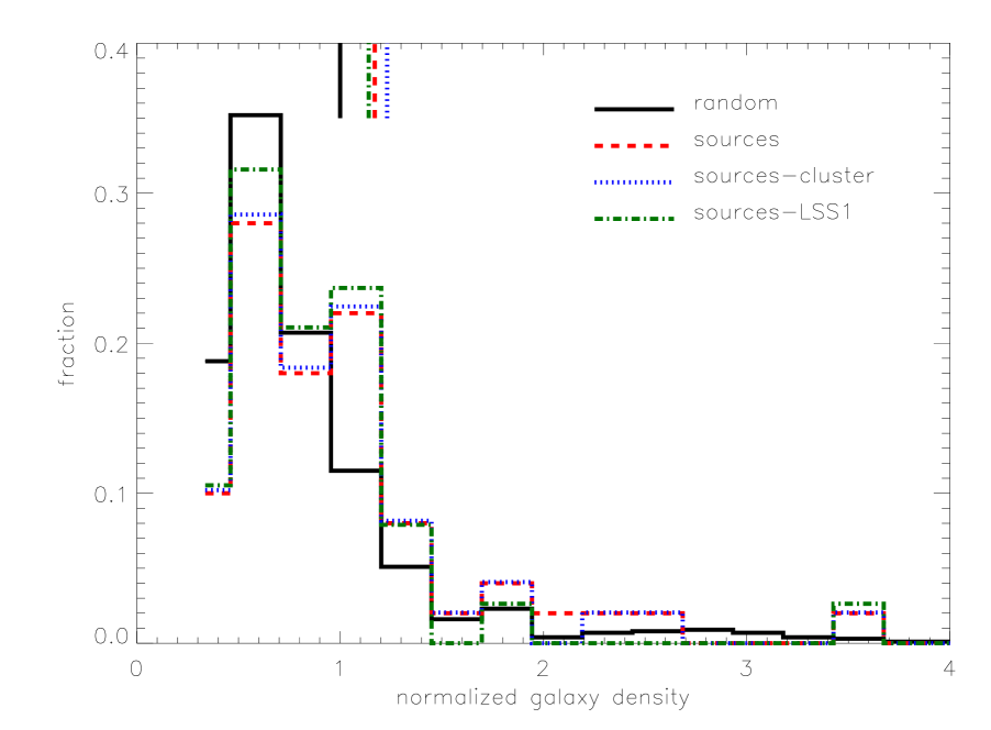
Figure 9: Histogram of the fraction of optical-IR selected galaxies at $0.60\mathrel{\lower 2.5pt\vbox{\hbox{$<$}\hbox{$\sim$}}}z\mathrel{\lower 2.5pt\vbox{\hbox{$<$}\hbox{$\sim$}}}0.67$ found within 30 arcsec of AzTEC source candidates (red dashed line), and around random positions within the AzTEC-mapped area of COSMOS (black solid line). The blue dotted-line histogram represents the number of optical-IR galaxies around AzTEC sources, excluding the single AzTEC source that falls within the X-ray traced cluster-outskirt region ($\theta\mathrel{\lower 2.5pt\vbox{\hbox{$<$}\hbox{$\sim$}}}1.5$ arcmin from the cluster centre, Guzzo et al., 2007), while the green dash-dotted histogram excludes the full 6 arcmin radial structure identified as Structure #1. The mean values of these histograms are represented at the top of the figure as vertical bars. The galaxy densities are normalised to the mean galaxy density in the full AzTEC-covered area such that the mean density of random positions is 1.

We next assess whether the substructures within Structure #1 are the main contributors to the observed correlation. Figure 9 shows the distribution of galaxy densities around AzTEC sources and around random positions in the collapsed $0.6\mathrel{\lower 2.5pt\vbox{\hbox{$<$}\hbox{$\sim$}}}z\mathrel{\lower 2.5pt\vbox{\hbox{$<$}\hbox{$\sim$}}}0.67$ map. The means differ at the 99.8% confidence level according to the MW $U$-test. If we exclude a circular region around the cluster centre with radius $\theta=1.5$’($\sim$ 0.6 Mpc), which contains both the cluster-core and the cluster-outskirt regions seen by the X-ray temperature profile (Guzzo et al., 2007), the significance of the difference is 99.94%. Excluding a larger circular region of radius $\theta=6$’($\sim$ 2.4 Mpc), which represents the FWHM of the full Structure #1, the MW significance decreases to only 98.6%. This demonstrates that although AzTEC sources do correlate with the galaxy densities associated with the extended Structure #1, the less prominent large-scale structure across the rest of the map is also well-correlated with the AzTEC positions.

Figure 10 shows the optical/IR galaxy density map for the redshift slice $0.24\mathrel{\lower 2.5pt\vbox{\hbox{$<$}\hbox{$\sim$}}}z\mathrel{\lower 2.5pt\vbox{\hbox{$<$}\hbox{$\sim$}}}0.26$, which is also a large contributor to the overall correlation between the large-scale-structure of the field and AzTEC sources (Figure 7). Structure #22 from Scoville et al. (2007), with $\sim 67$ possible galaxy members at $z\approx 0.26\pm 0.11$, is the main cluster in this redshift slice and is also detected in X-ray. However, as with the portion of Structure #1 in the $0.60\mathrel{\lower 2.5pt\vbox{\hbox{$<$}\hbox{$\sim$}}}z\mathrel{\lower 2.5pt\vbox{\hbox{$<$}\hbox{$\sim$}}}0.67$ slice, this system does not dominate the overall correlation with AzTEC sources: the mean galaxy density around AzTEC sources differs from random locations at the 99.1% level after exclusion of the $\Delta$ RA $\approx 0.06$ deg and $\Delta$ Dec $\approx 0.14$ deg area of influence of the cluster. Similarly, we find that the prominent contributions of other redshift slices (e.g. $z\sim 0.33$ and $z\sim 0.8$) to the overall spatial correlation are not due to single compact structures.

It appears that the observed correlations are not dominated by the clusters in the field, thus it is not surprising that the AzTEC positions are, in general, less correlated with the weak-lensing mass map of COSMOS (Massey et al., 2007), which is particularly sensitive to the most massive structures like the $z\approx 0.73$ cluster (see Figure 11). The null hypothesis that the distribution of masses found within 30” of AzTEC positions is the same as that found around random positions in the weak-lensing map is “rejected” at only the 60% level (K-S test), and their means differ at the 91.5% level (MW $U$-test).

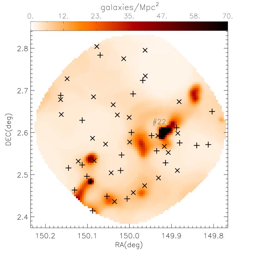
Figure 10: Smoothed surface density map of galaxies at $0.24\mathrel{\lower 2.5pt\vbox{\hbox{$<$}\hbox{$\sim$}}}z\mathrel{\lower 2.5pt\vbox{\hbox{$<$}\hbox{$\sim$}}}0.26$ detected at optical-IR wavelengths by the COSMOS survey, which includes Structure #22 of Scoville et al. (2007). Symbols are the same as in Figure 5

.

4 Discussion

The distribution of AzTEC sources is correlated with the large-scale distribution of optical/IR galaxies at $z\mathrel{\lower 2.5pt\vbox{\hbox{$<$}\hbox{$\sim$}}}1.1$ and the primary (but not unique) contributors to this signal are located at redshifts $0.60\mathrel{\lower 2.5pt\vbox{\hbox{$<$}\hbox{$\sim$}}}z\mathrel{\lower 2.5pt\vbox{\hbox{$<$}\hbox{$\sim$}}}0.65$ and $0.24\mathrel{\lower 2.5pt\vbox{\hbox{$<$}\hbox{$\sim$}}}z\mathrel{\lower 2.5pt\vbox{\hbox{$<$}\hbox{$\sim$}}}0.26$ (section § 3). The correlations in these redshift regimes are robust, with mean optical/IR densities differing from random distributions at the 99.1 to 99.98% level (MW $U$-test). For the seven AzTEC sources that have been followed up with SMA interferometry (Younger et al., 2007) and the additional 14 that have radio detections (Scott et al., 2008), secure optical/IR counterparts have been identified. The optical-IR and FIR-mm-radio photometric redshifts of these sources place the majority of these objects at $z\mathrel{\lower 2.5pt\vbox{\hbox{$>$}\hbox{$\sim$}}}3$; therefore, AzTEC detected sources are most likely background systems to the $z\mathrel{\lower 2.5pt\vbox{\hbox{$<$}\hbox{$\sim$}}}1.1$ galaxy densities shown in Figure 5. This is not surprising, given that the population of SCUBA SMGs with radio counterparts have a median redshift of 2.2 (Chapman et al., 2003, 2005; Aretxaga et al., 2003, 2007; Pope et al., 2005).

The amplification caused by massive clusters at intermediate redshifts ($z\sim 0.2-0.4$) has been used to detect and study the sub-millimetre galaxy population since the first SMG surveys (e.g. Smail et al., 1997). Lensing is expected to occur also in and around the $z\approx 0.73$ cluster detected in the COSMOS field, but only 4 of the 50 $S/N\geq 3.5$ AzTEC source-candidates are projected within 2’ of the dense cluster core. Removing these sources/regions from the analysis of § 3 has little effect on the correlation strength. Thus the correlations seem to be tied to the general $z\mathrel{\lower 2.5pt\vbox{\hbox{$<$}\hbox{$\sim$}}}1.1$ large-scale structure in the field. The same result holds if we exclude the other prominent structures in this field, Structures #24 at $z\approx 0.61$ and #22 at $z\approx 0.26$. Furthermore, the bulk of AzTEC sources do not significantly correlate with the weak-lensing map, which is particularly sensitive to the mass contained in rich clusters.

Lensing of the sub-mm galaxy population by foreground low-redshift structures has been claimed in the correlation analysis of 39 sub-millimetre galaxies detected in 3 disjoint fields with the density of $R<23$ mag galaxies (Almaini et al., 2005), which statistically lie at $\langle z\rangle\sim 0.5$. It was argued that the bright $S_{850\mu{\rm m}}>10$ mJy sources are found to cluster preferentially around the highest-density areas, and Almaini et al. (2005) estimate that 20-25% of the sub-millimetre galaxy population is subject to lensing by foreground structures. We note that a similar study performed in the GOODS-N region (Blake et al., 2006) found no detectable correlation between 35 SCUBA-selected SMGs and the optically-selected galaxy populations at $z\leq 0.8$. This difference in correlation strength may be related to cosmic variance of foreground structure on the scale of these maps. There also exist potential cases of lensing by individual galaxies, with some SCUBA sources being incorrectly identified as low-redshift galaxies due to intervening foreground galaxies that lie directly along the line of sight (Chapman et al., 2002; Dunlop et al., 2004). Since it includes a high-density region within the COSMOS field, the AzTEC survey is sensitive to all of these types of amplification, and we have demonstrated that there is a positive correlation with the large-scale structure. Inspection of the optical/IR counterparts of the 21 AzTEC galaxies with radio and/or sub-mm interferometric positional accuracy, including the 7 sources known to have sub-millimetre emission on scales $\theta<1.2$” (Younger et al., 2007), show no obvious signs of strong galaxy-galaxy lensing and hence any amplification of this sub-sample must be attributed to weak-lensing.

If our blank-field number counts model (§ 2.4) accurately represents the intrinsic (non-amplified) SMG population in the AzTEC/COSMOS field, then the observed number density of sources is also consistent with weak-lensing of the background SMG population. Parametric fits to the flux-corrected number counts (§ 2.3, see also Table 2 and Figure 3) show that the relative over-density of sources can be fully explained as a systematic increase in the parameter $S^{\prime}$, which is consistent with an average flux amplification (e.g. lensing) of the source population by $\sim$ 30%. Conversely, the number counts data are only marginally consistent with a simple increase in the normalisation parameter $N^{\ast}$, thus disfavouring a uniform physical over-density (e.g. cosmic variance) of sources in this field as the sole cause of the observed over-density. Additionally, any over-density due to variance and/or clustering can not explain the correlation of AzTEC sources to the $z\mathrel{\lower 2.5pt\vbox{\hbox{$<$}\hbox{$\sim$}}}1.1$ structure, as the AzTEC sources are likely background sources and not physically associated with the $z\mathrel{\lower 2.5pt\vbox{\hbox{$<$}\hbox{$\sim$}}}1.1$ structure.

An alternative cause of the number counts over-density can be imagined as an additive flux source (e.g. dense screen of faint foreground sources) confused with the blank-field sources. However, the AzTEC/COSMOS map has been filtered for point source detection and has a mean of zero (Scott et al., 2008), which leaves the map insensitive to high-density or uniform millimetre flux sources that span large spatial scales. Furthermore, the positions of AzTEC sources are not strongly correlated with the most dense and compact foreground regions (i.e. clusters) that could otherwise be potential sources of additional mm-wave flux in our map (e.g. the Sunyaev-Zel’dovich effect).

The significance of the spatial correlation between AzTEC sources and the intervening large-scale structure contrasts with the lack of a similar detectable signal among the sources discovered by COSBO (Bertoldi et al., 2007), the 1.2 mm MAMBO survey to the south and adjacent to the AzTEC surveyed area (see Figure 11). If we repeat the analysis performed in § 3 with the MAMBO catalogue, we do not find a significant correlation with the COSMOS optical/IR galaxy surface density; the probability that the galaxy densities around MAMBO sources are different from that around random positions in the map is only 87% (K-S test). This lack of a significant correlation signal may be due in part to the smaller catalogue of significant sources in the COSBO field and the overall lack of significant foreground structure in much of the COSBO covered area.

The association between COSBO sources and the weak-lensing derived mass-map, however, is stronger with a 99.4% probability (K-S test) that the distribution of mass around MAMBO source locations is different from that of random positions in the COSBO survey region. This signal is dominated by a group of $\sim 7-8$ of the most significant MAMBO sources close to two compact mass spikes, which are identified with X-ray bright over-densities consisting of a total of $\sim 127$ galaxies at $z\approx 0.24$ (Structure #17 in Scoville et al., 2007) and are likely clusters. The possible spatial correlation of COSBO sources with foreground structures, therefore, might be of a somewhat different nature than that of AzTEC sources. The COSBO region may be witnessing amplification caused by the two clusters revealed by the weak-lensing map, while the AzTEC sources are more likely amplified by galaxies contained within the more tenuous filamentary large-scale structure, which is so tenuous in the COSBO field that it provides no significant signal in the sample of MAMBO sources.

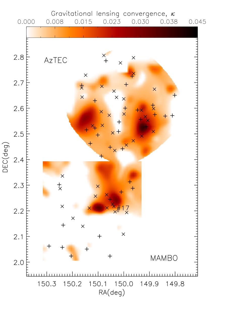
Figure 11: Weak-lensing convergence mass map (Massey et al., 2007) of the AzTEC and MAMBO surveyed regions of COSMOS. Crosses mark the millimetre source positions from the two catalogues and follow the notation of Figure 5.

5 Conclusions

The central 0.15 deg² of the AzTEC/COSMOS survey shows a significant over-density of bright 1.1 mm-detected SMGs when compared to the background population inferred by other surveys. We find that this over-density cannot be explained as sample variance of the blank-field SMG population. The SMG positions are significantly correlated with the $z\mathrel{\lower 2.5pt\vbox{\hbox{$<$}\hbox{$\sim$}}}$ 1.1 optical/IR galaxy density on the sky, which is believed to be in the foreground of nearly all AzTEC/COSMOS SMGs. Both the spatial correlation and the AzTEC/COSMOS SMG number counts are consistent with gravitational amplification of the blank-field SMG population. The lack of strong correlation to the weak-lensing maps of Massey et al. (2007) indicates that this amplification is primarily due to weak-lensing by the large-scale structure as opposed to lensing by the compact and massive clusters in the field. SMGs detected in a different part of the COSMOS field by the 1.2 mm COSBO survey are also spatially correlated to the $z\mathrel{\lower 2.5pt\vbox{\hbox{$<$}\hbox{$\sim$}}}$ 1.1 structure, however, this correlation is dominated by two compact structures (likely clusters) in the field. The lack of significant large-scale structure (i.e. lensing opportunities) in the rest of the COSBO survey region results in COSBO number counts that are consistent with the blank-field (Bertoldi et al., 2007) – a strong contrast to the significant SMG over-density and rich foreground structure found in the nearby AzTEC/COSMOS field.

References

- Almaini et al. (2005) Almaini O., Dunlop J. S., Willott C. J., Alexander D. M., Bauer F. E., Liu C. T., 2005, MNRAS, 358, 875
- Almaini et al. (2003) Almaini O., Scott S. E., Dunlop J. S., Manners J. C., Willott C. J., Lawrence A., Ivison R. J., Johnson O., Blain A. W., Peacock J. A., Oliver S. J., et al., 2003, MNRAS, 338, 303
- Aretxaga et al. (2003) Aretxaga I., Hughes D. H., Chapin E. L., Gaztañaga E., Dunlop J. S., Ivison R. J., 2003, MNRAS, 342, 759
- Aretxaga et al. (2007) Aretxaga I., Hughes D. H., Coppin K., Mortier A. M. J., Wagg J., Dunlop J. S., Chapin E. L., Eales S. A., Gaztañaga E., Halpern M., Ivison R. J., et al., 2007, MNRAS, 379, 1571
- Baugh et al. (2005) Baugh C. M., Lacey C. G., Frenk C. S., Granato G. L., Silva L., Bressan A., Benson A. J., Cole S., 2005, MNRAS, 356, 1191
- Bertoldi et al. (2007) Bertoldi F., Carilli C., Aravena M., Schinnerer E., Voss H., Smolcic V., Jahnke K., Scoville N., Blain A., Menten K. M., et al., 2007, ApJS, 172, 132
- Best (2002) Best P. N., 2002, MNRAS, 336, 1293
- Blake et al. (2006) Blake C., Pope A., Scott D., Mobasher B., 2006, MNRAS, 368, 732
- Borys et al. (2003) Borys C., Chapman S., Halpern M., Scott D., 2003, MNRAS, 344, 385
- Chapman et al. (2003) Chapman S. C., Blain A. W., Ivison R. J., Smail I. R., 2003, Nature, 422, 695
- Chapman et al. (2005) Chapman S. C., Blain A. W., Smail I., Ivison R. J., 2005, ApJ, 622, 772
- Chapman et al. (2002) Chapman S. C., Scott D., Borys C., Fahlman G. G., 2002, MNRAS, 330, 92
- Chapman et al. (2002) Chapman S. C., Smail I., Ivison R. J., Blain A. W., 2002, MNRAS, 335, L17
- Coppin et al. (2006) Coppin K., Chapin E. L., Mortier A. M. J., Scott S. E., Borys C., Dunlop J. S., Halpern M., Hughes D. H., Pope A., Scott D., et al., 2006, MNRAS, 372, 1621
- Coppin et al. (2005) Coppin K., Halpern M., Scott D., Borys C., Chapman S., 2005, MNRAS, 357, 1022
- Cowie et al. (2002) Cowie L. L., Barger A. J., Kneib J.-P., 2002, AJ, 123, 2197
- De Breuck et al. (2004) De Breuck C., Bertoldi F., Carilli C., Omont A., Venemans B., Röttgering H., Overzier R., Reuland M., Miley G., Ivison R., van Breugel W., 2004, A&A, 424, 1
- Dunlop et al. (2004) Dunlop J. S., McLure R. J., Yamada T., Kajisawa M., Peacock J. A., Mann R. G., Hughes D. H., Aretxaga I., Muxlow T. W. B., Richards A. M. S., Dickinson M., Ivison R. J., Smith G. P., Smail I., Serjeant S., Almaini O., Lawrence A., 2004, MNRAS, 350, 769
- Dunne et al. (2000) Dunne L., Eales S., Edmunds M., Ivison R., Alexander P., Clements D. L., 2000, MNRAS, 315, 115
- Dunne & Eales (2001) Dunne L., Eales S. A., 2001, MNRAS, 327, 697
- Fasano & Franceschini (1987) Fasano G., Franceschini A., 1987, MNRAS, 225, 155
- Granato et al. (2004) Granato G. L., De Zotti G., Silva L., Bressan A., Danese L., 2004, ApJ, 600, 580
- Greve et al. (2008) Greve T. R., Pope A., Scott D., Ivison R. J., Borys C., Conselice C. J., Bertoldi F., 2008, MNRAS, 389, 1489
- Greve et al. (2007) Greve T. R., Stern D., Ivison R. J., De Breuck C., Kovács A., Bertoldi F., 2007, MNRAS, 382, 48
- Griffin & Orton (1993) Griffin M. J., Orton G. S., 1993, Icarus, 105, 537
- Guzzo et al. (2007) Guzzo L., Cassata P., Finoguenov A., Massey R., Scoville N. Z., Capak P., Ellis R. S., Mobasher B., Taniguchi Y., Thompson D., Ajiki M., Aussel H., et al., 2007, ApJS, 172, 254
- Hogg & Turner (1998) Hogg D. W., Turner E. L., 1998, PASP, 110, 727
- Ilbert et al. (2008) Ilbert O., Capak P., Salvato M., Aussel H., McCracken H. J., Sanders D. B., Scoville N., Kartaltepe J., Arnouts S., Le Floc’h E., Mobasher B., et al., 2008, ArXiv e-prints
- Kaviani et al. (2003) Kaviani A., Haehnelt M. G., Kauffmann G., 2003, MNRAS, 340, 739
- Knudsen et al. (2006) Knudsen K. K., Barnard V. E., van der Werf P. P., Vielva P., Kneib J.-P., Blain A. W., Barreiro R. B., Ivison R. J., Smail I., Peacock J. A., 2006, MNRAS, 368, 487
- Laurent et al. (2005) Laurent G. T., Aguirre J. E., Glenn J., Ade P. A. R., Bock J. J., Edgington S. F., Goldin A., Golwala S. R., Haig D., Lange A. E., et al., 2005, ApJ, 623, 742
- Massey et al. (2007) Massey R., Rhodes J., Ellis R., Scoville N., Leauthaud A., Finoguenov A., Capak P., Bacon D., Aussel H., Kneib J.-P., Koekemoer A., McCracken H., et al., 2007, Nature, 445, 286
- Negrello et al. (2007) Negrello M., Perrotta F., González J. G.-N., Silva L., de Zotti G., Granato G. L., Baccigalupi C., Danese L., 2007, MNRAS, 377, 1557
- Peacock (1983) Peacock J. A., 1983, MNRAS, 202, 615
- Perera et al. (2008) Perera T. A., Chapin E. L., Austermann J. E., Scott K. S., Wilson G. W., Halpern M., Pope A., Scott D., Yun M. S., Lowenthal J. D., Morrison G., et al., 2008, MNRAS, in press
- Pope et al. (2005) Pope A., Borys C., Scott D., Conselice C., Dickinson M., Mobasher B., 2005, MNRAS, 358, 149
- Press et al. (1992) Press W. H., Teukolsky S. A., Vetterling W. T., Flannery B. P., 1992, Numerical recipes in C. The art of scientific computing. Cambridge: University Press, —c1992, 2nd ed.
- Priddey et al. (2008) Priddey R. S., Ivison R. J., Isaak K. G., 2008, MNRAS, 383, 289
- Schechter (1976) Schechter P., 1976, ApJ, 203, 297
- Scott et al. (2008) Scott K. S., Austermann J. E., Perera T. A., Wilson G. W., Aretxaga I., Bock J. J., Hughes D. H., Kang Y., Kim S., Mauskopf P. D., Sanders D. B., Scoville N., Yun M. S., 2008, MNRAS, 385, 2225
- Scott et al. (2006) Scott S. E., Dunlop J. S., Serjeant S., 2006, MNRAS, 370, 1057
- Scoville et al. (2007) Scoville N., Aussel H., Benson A., Blain A., Calzetti D., Capak P., Ellis R. S., El-Zant A., Finoguenov A., Giavalisco M., et al., 2007, ApJS, 172, 150
- Scoville et al. (2007) Scoville N., Aussel H., Brusa M., Capak P., Carollo C. M., Elvis M., Giavalisco M., Guzzo L., Hasinger G., Impey C., et al., 2007, ApJS, 172, 1
- Smail et al. (1997) Smail I., Ivison R. J., Blain A. W., 1997, ApJ, 490, L5+
- Smail et al. (2002) Smail I., Ivison R. J., Blain A. W., Kneib J.-P., 2002, MNRAS, 331, 495
- Stevens et al. (2003) Stevens J. A., Ivison R. J., Dunlop J. S., Smail I. R., Percival W. J., Hughes D. H., Röttgering H. J. A., van Breugel W. J. M., Reuland M., 2003, Nature, 425, 264
- Valiante et al. (2007) Valiante E., Lutz D., Sturm E., Genzel R., Tacconi L. J., Lehnert M. D., Baker A. J., 2007, ApJ, 660, 1060
- Webb et al. (2005) Webb T. M. A., Yee H. K. C., Ivison R. J., Hoekstra H., Gladders M. D., Barrientos L. F., Hsieh B. C., 2005, ApJ, 631, 187
- Wilson et al. (2008) Wilson G. W., Aretxaga I., Hughes D., Ezawa H., Austermann J. E., Doyle S., Hernandez-Curiel I., Kawabe R., Kitayama T., Kohno K., Kuboi A., et al., 2008, MNRAS, in press
- Wilson et al. (2008) Wilson G. W., Austermann J. E., Perera T. A., Scott K. S., Ade P. A. R., Bock J. J., Glenn J., Golwala S. R., Kim S., Kang Y., Lydon D., Mauskopf P. D., Predmore C. R., Roberts C. M., Souccar K., Yun M. S., 2008, MNRAS, 386, 807
- Younger et al. (2007) Younger J. D., Fazio G. G., Huang J.-S., Yun M. S., Wilson G. W., Ashby M. L. N., Gurwell M. A., Lai K., Peck A. B., Petitpas G. R., Wilner D. J., et al., 2007, ApJ, 671, 1531
- Yun et al. (2008) Yun M. S., Aretxaga I., Ashby M. L. N., Austermann J., Fazio G. G., Giavalisco M., Huang J. ., Hughes D. H., Kim S., Lowenthal J. D., Perera T., Scott K., Wilson G. W., Younger J. D., 2008, MNRAS, in press