Characterization of the HD 17156 planetary system

Abstract

Aims. To improve the parameters of the HD 17156 system (peculiar due to the eccentric and long orbital period of its transiting planet) and constrain the presence of stellar companions.

Methods. Photometric data were acquired for 4 transits, and high precision radial velocity measurements were simultaneously acquired with SARG@TNG for one transit. The template spectra of HD 17156 was used to derive effective temperature, gravity, and metallicity. A fit of the photometric and spectroscopic data was performed to measure the stellar and planetary radii, and the spin-orbit alignment. Planet orbital elements and ephemeris were derived from the fit. Near infrared adaptive optic images was acquired with ADOPT@TNG.

Results. We have found that the star has a radius of R${}_{S}=1.44\pm 0.03$R_⊙ and the planet R${}_{P}=1.02\pm 0.08$R_J. The transit ephemeris is T${}_{c}=2\,454\,756.73134\pm 0.00020+N\cdot 21.21663\pm 0.00045$ BJD. The analysis of the Rossiter-Mclaughlin effect shows that the system is spin orbit aligned with an angle $\lambda=4.8^{\circ}\pm 5.3^{\circ}$. The analysis of high resolution images has not revealed any stellar companion with projected separation between 150 and 1 000 AU from HD 17156.

1 Introduction

The discovery of transiting extrasolar planets (TESP) is of special relevance for the study and characterization of planetary systems. The combination of photometric and radial velocity measurements allows to measure directly the mass and radius of an exoplanet, and hence its density, which is the primary constraint on a planet’s bulk composition. Dedicated follow-up observations of TESP during primary transit and secondary eclipse at visible as well as infrared wavelengths allow direct measurements of planetary emission and absorption (e.g., Charbonneau et al. (2007), and references therein). Transmission spectroscopy during primary eclipse in recent years has been successful in characterizing the atmospheric chemistry of several Hot Jupiters (e.g., Charbonneau et al. (2002) and Tinetti et al. (2007)). Infrared measurements gathered at a variety of orbital phases, including secondary eclipse, have permitted the characterization of the longitudinal temperature profiles of nearby TESP. The quickly increasing amount of high-quality data obtained for TESP has provided the first crucial constraints on theoretical models describing the physical structure and the atmospheres of gas and ice exoplanets. The detailed characterization of TESP ultimately is of special relevance to test several proposed formation and orbital evolution mechanisms of close-in planets.

The planet HD~17156b, detected by Fischer et al. (2007)(hereinafter F07) using the radial velocity method, was shown to transit in front of its parent star by Barbieri et al. (2007). Additional photometric measurements were presented in follow-up papers by Gillon et al. (2008), Narita et al. (2008), Irwin et al. (2008), Winn et al. (2008). This planet is unique among the known transiting systems in that its period (21.2 days) is more than 5 times longer than the average period for this sample, and it has the largest eccentricity ($e=0.67$).

Schlesinger (1910), Rossiter (1924) and McLaughlin (1924) showed that a transiting object, like a stellar companion, produces a distortion in the stellar line profiles due to the partial eclipse of the rotating stellar surface during the event, and thus an apparent anomaly in the measured radial velocity of the observed primary star. In the case of close-in giant planets transiting solar-type stars, the amplitude of the Rossiter-McLaughlin effect ranges typically between a few and $\sim 100$ m s^-1, depending on orbital period, stellar and planetary radii, and stellar rotational velocity. This is within the current instrument capabilities for the brightest transiting planets. Indeed, this effect has been previously observed on several TESP (e.g. Winn (2008) and references therein). The observation of the Rossiter-McLaughlin effect allows to measure the relative inclination angle between the sky projections of the orbital plane and the stellar spin axis. Another important result derived from these observations is the possibility to determine whether short orbital period transiting planets move in the same direction of the stellar spin, indicating the existence of strong dynamical interactions between the parent star and its planet. Measurements of the Rossiter-McLaughlin effect thus provide relevant fossil evidence of planet formation and migration processes, as well as dynamical interactions with perturbing bodies (Marzari & Weidenschilling, 2002)

Up to now 8 of the 9 transiting planets for which the Rossiter-McLaughlin effect was measured are coplanar systems, as our Solar System (the orbital axes of all the planets and the Sun spin axis are aligned within a few degrees). This is compatible with a formation mechanism for close-in giant planets including migration via tidal interactions with the protoplanetary disk. Only the XO-3 planet seems to be a non aligned system (Hébrard et al., 2008).

The measurement of the Rossiter-McLaughlin effect is of special relevance for the HD~17156 system, given the very high eccentricity and orbital period, much longer than the other transiting planets. With a period of 21 days, HD~17156b is well outside the peak in the period distribution of close-in planets at about 3 days, possibly implying a different migration history with respect to the other transiting planets. An eccentricity as high as that of HD~17156b can be hardly explained by models of planet migration via tidal interactions with the protoplanetary disk. Alternatively, high-eccentricity planets might be the outcome of a variety of possible planet-planet dynamical interactions (Marzari & Weidenschilling, 2002). In these scenarios, high relative inclinations between the stellar rotation axis and the planet orbit plane are possible. An additional way to get large relative inclinations and eccentricities is represented by Kozai resonances with close stellar companion. Interestingly, a rather large planetary mass coupled with a short orbital period might be an indication for binarity, as typically high-mass short-period planets occur in binary systems (Desidera & Barbieri, 2007).

Narita et al. (2008) presented the first observations of the Rossiter-McLaughlin effect in HD~17156. They found an angle between the sky projections of the orbital axis and the stellar rotation axis $\lambda=62\pm 25^{\circ}$. However, Cochran et al. (2008) did not confirm this claim, suggesting instead well-aligned axes. Such a discrepancy calls for additional high-precision RV monitoring during planetary transit. These are presented in this work, along with additional photometric observations and a critical revision of stellar and planetary parameters. To further constrain the origin of the special properties of HD 17156b , we also searched for possible wide stellar companions using adaptive optics observations.

The overall organization of this paper begins in Sec. 2 with the description of high resolution spectroscopy data obtained with SARG@TNG. The following Sec.3 covers the analysis of the stellar parameters. Sec.4 presents the photometric data collected during several planetary transits. Next Sec.5 describes the analysis of the radial velocity and photometric data, and their results. In Sec.6 we present the results for the search of additional stellar companions to HD 17156 . Finally in Sec.7 our conclusion are presented.

2 High resolution spectroscopy

We observed HD 17156 on 2007 December 3, including continuous monitoring (about 8 hours) during the transit, with SARG, the high resolution spectrograph of the TNG (Gratton et al., 2001). Observing conditions were not optimal, with seeing ranging from 1.3″to 2.0 ″. We obtained the stellar template (without the iodine cell) first and then started the uninterrupted series of observations with the iodine cell. Exposure time of the spectra acquired with the iodine cell was 900 s, typically resulting in S/N of about 80 per pixel. One additional spectrum was obtained on 25 Oct 2007. These spectra were reduced and analyzed as those for the ongoing planet search program with SARG (Desidera et al., 2007) using the AUSTRAL code (Endl et al., 2000). Table 1 lists the radial velocities.

Table 1: Differential radial velocities and bisector velocity span of HD 17156 obtained with SARG at TNG.

BJD	RV	err	span	err
	m/s	m/s	m/s	m/s
2454398.58856	-81.03	5.76
2454438.40203	100.47	4.55	-25.47	63.07
2454438.41331	82.40	4.56	-32.78	62.90
2454438.42460	76.72	4.55	19.04	60.32
2454438.43608	90.10	4.43	74.70	59.30
2454438.44737	91.46	3.98	-5.58	56.75
2454438.45866	76.28	4.35	64.69	59.89
2454438.47011	65.86	3.98	47.68	57.10
2454438.48140	60.08	4.01	40.49	53.96
2454438.49270	30.74	3.72	119.82	57.44
2454438.50415	32.97	3.98	216.98	59.74
2454438.51544	20.63	4.49	108.08	57.92
2454438.52671	18.78	4.59	74.54	57.66
2454438.53816	4.29	4.29	82.66	58.07
2454438.54946	-3.77	4.13	90.90	57.79
2454438.56075	7.21	4.93	41.59	63.36
2454438.57218	-3.84	3.77	58.41	57.50
2454438.58349	-11.52	4.53	50.75	60.76
2454438.59478	-31.71	4.43	45.47	59.96
2454438.62486	-26.61	4.74	36.70	64.19
2454438.63615	-43.01	4.01	18.82	58.87
2454438.64745	-46.79	4.23	66.00	65.44
2454438.65894	-54.19	4.77	-38.79	65.29
2454438.67023	-55.35	4.72	3.19	67.30
2454438.68152	-64.85	5.32	102.93	70.23
2454438.69306	-71.94	5.20	73.98	67.86
2454438.70435	-82.48	5.08	111.26	72.47
2454438.71584	-88.29	5.13	-18.92	72.31
2454438.72713	-92.59	5.15	94.27	72.55

The absolute radial velocity of HD 17156 was derived by cross correlating the stellar template acquired with SARG to a few suitable reference stars observed with the same set-up and with available high-accuracy absolute radial velocity from Nidever et al. (2002). It results in $-3.15\pm 0.20$ km/s.

3 Stellar parameters

3.1 Spectroscopic analysis

We have used the TNG/SARG template spectrum of HD 17156 to provide an independent assessment of its atmospheric parameters ($T_{\rm eff}$, $\log{g}$, and [Fe/H]) with respect to the values reported by F07.

Our methodology follows a standard procedure whose details can be found in several works of the recent past  (e.g., Gonzalez & Lambert, 1996; Gonzalez et al., 2001; Santos et al., 2004). We briefly summarize it here. We initially selected a set of relatively weak Fe I and Fe II lines  (see, e.g., Sozzetti et al., 2004, and references therein, for details on the line list), and measured equivalent widths (EWs) using the automated software ARES , made available to the community by Sousa et al. (2007). The EWs measured with ARES are then fed to the 2002 version of the MOOG spectral synthesis code (Sneden, 1973) , together with a grid of Kurucz ATLAS plane-parallel stellar model atmospheres (Kurucz, 1993).

The atmospheric parameters of HD 17156 are then derived under the assumption of local thermodynamic equilibrium, using a standard technique of Fe ionization balance (see, e.g., Santos et al., 2004; Sozzetti et al., 2004, and references therein). We obtained $T_{\rm eff}$ $=6100\pm 75$ K, $\log{g}$ $=4.1\pm 0.1$, and [Fe/H]$=+0.14\pm 0.08$, the formal errors on $T_{\rm eff}$  and $\log{g}$  having been derived using the procedure described in Neuforge-Verheecke & Magain (1997) and Gonzalez & Vanture (1998), while the nominal uncertainty for [Fe/H] corresponds to the scatter obtained from the Fe I lines rather than the formal error of the mean.

We also quantified the sensitivity of our iron abundance determination to variations of $\pm 1\sigma$ with respect to the nominal $T_{\mathrm{eff}}$, and $\log g$ values, and found changes in [Fe/H] of at most 0.05 dex, below the adopted uncertainty of 0.08 dex.

With the aim of further testing the accuracy of the $T_{\rm eff}$  determination above, we have carried out a few additional consistency checks. For example, in Figure 1 we show the comparison of the observed H_α line profile in an archival Keck/HIRES spectrum against four synthetic profiles for solar-metallicity dwarfs ([Fe/H] = 0.0, $\log g=4.5$) from the Kurucz database. As is well-known, the H_α line is very sensitive to changes in $T_{\rm eff}$, while relatively insensitive to changes in $\log{g}$  and [Fe/H]  (see, e.g., Santos et al., 2006; Sozzetti et al., 2007, and references therein), thus this exercise certainly helps to test the accuracy of the spectroscopic $T_{\rm eff}$  derived above. The results shown in Figure 1, in which a 10 Å region centered on H_α is displayed together with four calculated profiles for different $T_{\rm eff}$  values, indicate rather good agreement with the estimate reported in Table 2.

Figure 1: The portion of the spectrum of HD 17156 around H_α and synthetic profiles for four different $T_{\rm eff}$. A $T_{\rm eff}$ close to 6000 K is suggested by the fit of the wings of the line.

3.2 Age

Based on isochrone fitting, F07 reported an age estimate for HD 17156 of 5.7${}^{+1.3}_{-1.9}$ Gyr, suggesting an old, slightly evolved F8/G0 primary. We performed an independent isochrone fitting using the set of isochrones of Girardi et al. (2000) and the software PARAM described in da Silva et al. (2006). The input values for PARAM are the parallax, the visual magnitude, [Fe/H] and $T_{\rm eff}$. We used the parallax from van Leeuwen (2007) and for the metallicity and effective temperature we ran the code twice, once with the values from F07 and once with our estimate. The results of PARAM for the stellar age are 2.4 $\pm 1$ and 2.8 $\pm 1$ Gyr, for the F07 and our parameters, respectively. These are only marginally compatible with the previous age estimate by F07. The stellar mass and radius are instead fully compatible (see below).

Other indirect age indicators confirm an age of a few Gyr. The low level of Ca II H&K chromospheric activity suggests an age of about 6 Gyr (Fischer et al., 2007). The lack of X-ray emission from ROSAT (Voges et al., 2000) yields an upper limit of $\log L_{X}<28.7$. This in turn implies an age older than 1.6 Gyr, using the age-X ray emission calibration by Mamajek & Hillenbrand (2008).

To obtain an additional age estimate and to investigate possible chemical peculiarities of HD 17156 with respect to other planet hosts with similar physical properties, we have measured its lithium (Li) abundance.

Figure 2 shows a spectral synthesis of a 10 Å region centered on the Li  $\lambda=$ 6707.8 Å line in an archival Keck/HIRES spectrum of HD 17156 , and using the atmospheric parameters derived from the Fe-line analysis and the line list of Reddy et al. (2002). In the figure, the observed spectrum is compared to three synthetic spectra, each differing only in the assumed Li abundance. We find a best-fit value of $\log\epsilon{\rm(Li)}\approx 2.80$ for HD 17156 . We then infer a rather old age for the star of $t>2$ Gyr, based on the average Li abundance curves as a function of effective temperature for clusters of different ages reported by Sestito & Randich (2005).

The measured Li abundance for HD 17156 does not appear peculiar when compared to that of sub-samples of nearby planet hosts with similar $T_{\rm eff}$  (Israelian et al., 2004; Gonzalez, 2008). To further investigate these issues we will present in a future paper a more detailed study of the elemental abundances in HD 17156 .

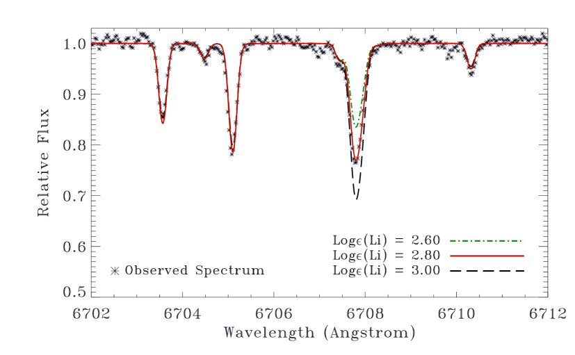
Figure 2: Portion of HD 17156 spectrum centered on Lithium 6707.8 Å line. Overplotted the results of the spectral synthesis for three different lithium abundance.

3.3 Stellar mass and radius

F07 provided mass and radius estimate from isochrone interpolations (mass 1.2 $\pm 0.1$ M_⊙, radius 1.47${}^{+0.13}_{-0.17}$ R_⊙). Our isochrone fit (see Sect. 3.2) gives 1.21 $\pm 0.03$ and 1.19 $\pm 0.03$ M_⊙ when assuming $T_{\rm eff}$ and [Fe/H] from the F07 and our analysis respectively, and same radius 1.35 $\pm 0.08$ R_⊙

The comparison of the results of the two fits show that they are compatible within error bars, but the best value are slightly different. The origin of these differences is not univocal, and to understand this problematic independent measurements of the star mass and radii are needed.

3.3.1 Monte Carlo experiment. Method

For this purpose we adopted an approach based on a Monte Carlo experiment. In each realization we generated a set of observed stellar properties. Using using calibrations from the literature we obtained the corresponding values for mass and radius. From the resulting distributions we obtained the most probable values and relative errors for the mass and radius.

In more detail, we created 10⁶ different synthetic systems where we generated Gaussian distributions for the parallax, the V and K magnitudes, and $T_{\rm eff}$, using as standard deviations their respectively error bars. The input parameters and relative their standard deviations are reported in Tab. 2. In the same way, we generated values for the bolometric correction and the bolometric magnitude of the Sun. For each synthetic set obtained this way we calculated the absolute magnitudes, luminosity, radius, mass, density and gravity.

The V magnitude was obtained from Simbad, K magnitude from 2MASS after conversion to the Bessel-Brett system (Carpenter, 2001), and the $T_{\rm eff}$ from our spectroscopic determination. For the parallax we adopted the recently revised Hipparcos value (van Leeuwen, 2007), which indicates that HD 17156 lies at 75 pc from the Sun, 3 pc closer than the previous estimate. The bolometric correction was set to B.C.$=-0.03$ (Girardi et al., 2000) while for the solar bolometric magnitude we used the value M${}_{bol,\odot}=4.77\pm$0.02.

The stellar radius was obtained using the $T_{\rm eff}$-K mag calibration of Kervella et al. (2004), and using the Stefan-Boltzmann law. The stellar mass was calculated from various mass-luminosity relations (MLR) namely: i) the classical MLR $L\propto M^{4.5}$; ii) the MLR of Malkov (2007) using absolute magnitude and ;iii) stellar luminosity; iv) the MLR of Henry (2004). Density and gravity were estimated directly from the radius and mass assuming a spherically symmetric star.

3.3.2 Monte Carlo experiment. Results

The distribution of absolute magnitudes in V band peaks at 3.7 (Fig. 3, upper left), while the luminosity is peaked at 2.5 L_⊙ (Fig. 3, upper right). These values are slightly different from the ones obtained by Fischer et al., and the source of these differences is ascribed only to the difference in the adopted parallax.

The resulting distributions for the radius are shown in Fig. 3 (middle left). The two relations used provide similar results (R${}_{S}\sim 1.4$R_⊙) for the best value and also the shape of the distributions is very similar. Fischer et al. suggest a slightly larger radius. Also in this case, the difference originates from the change in the adopted parallax.

In Fig. 3 (middle right) we present the mass distributions obtained with the MLRs. Using the relation of Henry (2004) we obtain the highest mass (M $\sim 1.28$M_⊙). However, we note that this relation was originally derived from parameters of close binary stars. Malkov (2003) demonstrated that this kind of relations do not well describe single stars. In order to avoid this problem we adopted the MLRs of Malkov (2007) obtained on detached main-sequence double-lined eclipsing binaries. These relations are also valid for slightly evolved stars like HD 17156 (almost all the stars used for deriving these relations are also slightly evolved. O. Malkov, private communication). We obtain best values for the mass between 1.2 and 1.24 M_⊙ , the first obtained using MLR($M_{V}$) and the second using MLR($L$). The classical MLR ($M\propto L^{4.5}$) provides M $\sim$1.22 M_⊙. These results are consistent with the values estimated by F07 (1.2 $\pm$ 0.1 M_⊙).

Finally, the resulting distributions for the gravity and the density are portrayed in the lower panels of Fig. 3. The mean values are $\log{g}$ = 4.22 and $\rho$ = 0.58 g /cm³.

The results of this experiment show a fairly good agreement with the estimate of R_S based on isochrone fitting (both our and the one by F07). We conclude that the two independent approaches based on isochrone fitting and the use of scaling relations provide consistent results.

In the following we do not adopt a value for the radius, because we want to determine independently its value from the light-curve fits. Moreover, we fix the value of the mass to the value of the weighted mean of our mass estimation (not using the Henry MLR results) M = 1.24$\pm$0.03 M_⊙. We summarize in Table 2 all the data relative to this Monte Carlo experiment.

Table 2: Upper panel Input parameters for the Monte Carlo experiment and best values. Lower panel Kinematical properties and galactic orbit parameters.

Monte Carlo experiment
Input parameters
parallax	13.33$\pm$ 0.72	mas
mag V	8.172 $\pm$ 0.031	mag
mag K	6.807 $\pm$ 0.024	mag
$T_{\rm eff}$	6100 $\pm$ 75	K
B.C.	-0.03 $\pm$ 0.02	mag
Output parameters
Mbol,⊙	3.69 $\pm$ 0.12	mag
MV	3.73 $\pm$ 0.12	mag
L	2.68 $\pm 0.28$	L⊙
R (Stefan-Boltzmann)	1.49 $\pm 0.09$	R⊙
R (Kervella)	1.45 $\pm 0.07$	R⊙
M (Malkov,MV)	1.21 $\pm 0.04$	M⊙
M (Malkov,L)	1.25 $\pm 0.04$	M⊙
M ($M\propto L^{4.5}$)	1.22 $\pm 0.04$	M⊙
M (Henry,MV)	1.29 $\pm 0.03$	M⊙
$\log{g}$ (mean)	4.21 $\pm 0.05$	cgs
$\rho$ (mean)	0.57 $\pm 0.10$	g /cm3
Kinematical properties
RV	-3.15 $\pm$ 0.2	$\rm km\,/s$
$\mu_{\alpha}$	91.14 $\pm$ 0.49	mas/yr
$\mu_{\delta}$	-33.14 $\pm$ 0.56	mas/yr
U	0.6 $\pm$ 0.2	$\rm km\,/s$
V	26.1 $\pm$ 2.0	$\rm km\,/s$
W	-22.8 $\pm$ 1.5	$\rm km\,/s$
Rmin	8.0 $\pm$ 0.3	kpc
Rmax	10.9 $\pm$ 0.3	kpc
Rmed	9.5 $\pm$ 0.4	kpc
Zmax	0.2 $\pm$ 0.1	kpc
e (galactic orbit)	0.15 $\pm$ 0.05

Figure 3: Probability density function of the stellar parameters obtained with the Monte Carlo experiment. Upper left: Absolute magnitude Upper right: Luminosity Middle left: Radius: thick line results using Stefan-Boltzmann law, thin line results using the calibration of Kervella($T_{\rm eff}$,M_K) Middle right: Mass, from left to right results using: Malkov MLR(M_V), $M\propto L^{4.5}$, Malkov MLR(L), and Henry MLR(M_V) Lower left: $\log{g}$ Lower right: Density

3.4 Rotational velocity

F07 derived v$\sin i=2.6\pm 0.5$ km/s for HD 17156 . Our template spectrum is suitable for an independent measurement of this quantity. We discuss here three different methods adopted for the measurements of v$\sin i$, based on our template spectra.

With the first method we derive v$\sin i$ by the Fast Fourier Transform analysis of the star’s absorption profile (see Fig.4). To determine the $v\sin i$, the observed profile of a stellar absorption line is made symmetric by mirroring one of its halves, with the purpose to reduce the noise of the FFT. A new profile is calculated by the convolution of a macroturbulence profile (Gaussian) and a rotational one, to compare the FFTs of the symmetric and the calculated (model) profiles. The v$\sin i$ value of the rotation profile, is set as variable parameter until the first minimum of the FFT from the calculated profile coincides with the minimum of the FFT from the symmetric one. The value of v$\sin i$ for HD 17156 was determined considering possible values of macroturbulent velocity ($v_{mac}$) from B-V and $T_{\rm eff}$ (Valenti & Fischer, 2005), and we obtained a v$\sin i$ ranging from 1.8 to 2.8 $\rm km\,/s$.

The second method that we used consists in obtaining the rotational velocity by means of a suitable calibration of the FWHM of the cross-correlation function against the B-V color. This relation was derived for all the stars in the SARG planet search survey, and it was calibrated into v$\sin i$ using stars with known rotational velocity from the literature. Using the B-V from the Tycho catalog converted to the Johnson system (B-V=0.632), the resulting v$\sin i$ $=3.2\pm 1$ $\rm km\,/s$ .

Finally, using MOOG we synthesized a number of isolated Fe I lines in the template spectrum. From these we measured v$\sin i$ $=3.0\pm 0.5$ $\rm km\,/s$.

The values obtained with the three methods suggest a range of values for v$\sin i$ compatible with the measurement of F07. The measurement of v$\sin i$ from the analysis of Rossiter-Mclaughlin effect will be presented in Section 5.3.

Figure 4: Estimation of v$\sin i$ through the FFT. Three profiles were analyzed: the observed profile (solid line), the symmetric profile (dashed line) mirroring one half of the profile, and a theoretical profile (dotted line). The FFT corresponds to a case considering $T_{eff}=6079$ K and Eq. 1 given by (Valenti & Fischer, 2005).

3.5 Galactic orbit

The measurements of the absolute radial velocity given in Section 2, together with the revised parallax and proper motion from Hipparcos van Leeuwen (2007), allow one to calculate the space velocity with respect to the Local Standard of Rest and the galactic orbit of HD 17156 . Space velocities are calculated following the procedure delineated by Johnson & Soderblom (1987) and Murray (1989), adopting the value of standard solar motion of Dehnen & Binney (1998) (with U positive toward the galactic anticenter). The calculations yield $(U,V,W)=(+0.6,+26.1,-22.8)$ $\rm km\,/s$. The galactic orbit of the star is obtained integrating the equations of motion of a massless particle in the potential described by Allen & Santillan (1991). The equations of motion are solved using the RADAU integrator (Everhart, 1985) assuming that the rectangular galactocentric coordinates of the Sun are $(X_{\odot},Y_{\odot},Z_{\odot})=(8.0,0.0,0.015)$ kpc, and that the local circular velocity is 220 km s^-1. We compute 1 000 orbits each time varying randomly the initial coordinates and velocity of the star within the error bars and integrating for a time of 4 Gyr ($\approx$ 15 full orbits around the Galactic Center). The UVW spatial velocity and the mean values of the computed orbits are reported in Table 2. The mean galactic radius provides an estimate of the galactocentric distance of the star at the moment of its formation. The value for HD 17156 , $R_{\mathrm{med}}=9.5$ kpc, implies that the star spends most of its time in regions outside of the solar circle.

4 Photometric observations

Photometric observations of the transit of 2007 December 3 were obtained with various telescopes. On 2007 December 2 we used three medium-class telescopes (Asiago 1.82 m and OHP 1.20 m) and a number of small telescopes, including six 30-40 cm amateur-operated telescope all located in continental Europe as well as the Telast 0.3-m telescope in the Canary Islands. Weather conditions across continental Europe were not optimal.

Observations at Asiago started under photometric conditions, transit ingress was observed but observations ended at December 04 UT 02:30, due to the presence of clouds, which prevented the observations of the third and fourth contacts. OHP observations were performed under variable sky conditions due to intermittent clouds and veils, good observing conditions were achieved only during the transit time window, with only a small coverage of the Out Of Transit (OOT) flat part of the lightcurve before the first contact. Observations with Telast were obtained under normal sky conditions and were performed throughout the night. Amateur observations were carried out by six observatories spread over central and northern Italy. Observing conditions suffered from clouds and veils as the others European sites involved in the campaign, and the full transit was successfully observed by four telescopes, the remaining two observatories obtaining data only for the ingress phase of the transit.

Three additional attempts to coordinate transit observations of HD 17156b were carried out on 25 December 2007 and on September 25 and October 17 2008. Unfortunately, due to bad weather conditions, there was only one useful observation for each date.

All observations were obtained in R band except the two obtained by B. Gary that was acquired in white light; the characteristics of the different telescopes are summarized in Table 3.

4.1 Data reduction

The Asiago, OHP, and Telast raw images were calibrated using flat field and bias frames. The resulting images were analyzed with IDL routines to perform standard aperture photometry. The center of the aperture was calculated using a Gaussian fit, and the aperture radius was held fixed for each set (in the range 15-20 pixels). The sky background contribution was removed after an estimation The brightest non-variable stars in the field were measured in the same way, and a reference light curve was constructed by adding the flux of these stars. The target flux was divided by this reference to get the final normalized light-curve.

The images obtained by amateur telescopes were reduced bias subtracted, and dark flat-field corrected using commercial software. Aperture photometry of HD 17156 was then performed using IRIS and adopting a fixed aperture equal to 2 times the stellar FWHM. The sum of the flux of the brightest stars in the field was used as reference for building the normalized light-curve.

The final light-curve for each telescope was corrected for differential airmass and residual systematic effects dividing them by a linear function of time to the region outside the transit. The photometric error on each point of a lightcurve was calculated as the rms over an interval of 30 minutes (the timescale of the ingress/egress phase). The typical rms of the OOT lightcurves are reported in Table 3, while the complete photometric dataset will be available in electronic format at CDS.

The whole dataset consists of $\sim$ 7 000 photometric points. We used these data to perform a global analysis of the planetary transit.

For the light curve fitting we used all the lightcurves that we have collected without performing data binning. In Fig.5 are portrayed the light curves used in this study, folded with the best orbital period from the fit. For displaying purposes the combined light-curve of the 15 lightcurves is shown in Fig. 6. This combined light curve was obtained using a bin width of 90 s, the OOT has an rms of 0.0016.

Table 3: Summary of photometric observations of HD 17156 performed on 2007/08. The last column report the midtransit times for each date obtained from the fit in Sec 5.2.

Site/Observer	diameter	rms OOT	date	Tc
	m	mmag		BJD
Telast	0.30	4.2	2007 September 10	2454353.61300 $\pm$ 0.0200
Gasparri	0.20	5.3
Lopresti	0.18	7.0
Asiago	1.82	2.8	2007 December 03	2454438.47450 $\pm$ 0.0005
OHP	1.2	2.0
Telast	0.3	11.2
Obs. Cavezzo	0.4	6.1
Lopresti	0.18	10.5
Obs. Univ.Siena	0.3	8.4
Obs. Mt. Baldo	0.4	7.3
Papini	0.3	6.9
Vallerani	0.25	5.9
Gary	0.3	5.6	2007 December 25	2454459.69087 $\pm$ 0.0032
Gregorio	0.3	3.8	2008 September 25	2454735.51351 $\pm$ 0.0027
Gary	0.3	8.9	2008 October 17	2454756.73134 $\pm$ 0.0024

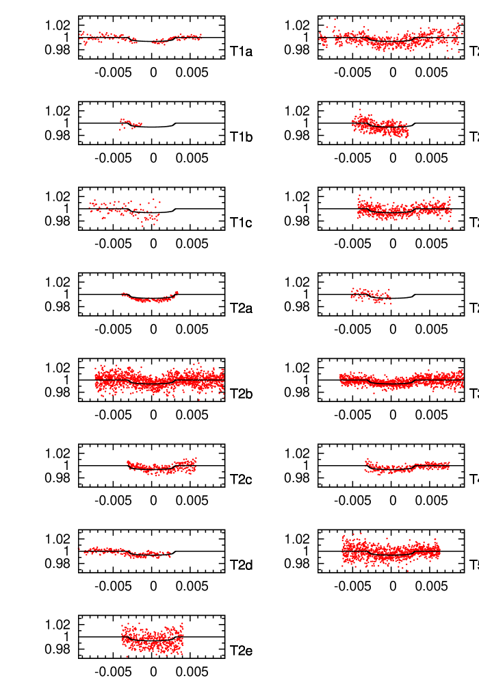
Figure 5: Mosaic of the differential light curves obtained during transits of HD 17156b . obtained with several telescopes. In each box the horizontal axis is the photometric phase and the vertical axis is the relative flux, along with the best fit model. From left to right column and from top to bottom: T1a=Almenara, T1b=Gasparri and T1c=Lopresti datasets from the Barbieri et al. (2007). T2a=OHP, T2b=Telast, T2c=Castellani, T2d=Asiago, T2e=Lopresti, T2f=Marchini, T2g=Nicolini, T2h=Papini, T2i=Vallerani. T2a to T2i light-curves were collected on 2007 December 03. T3a=Gary 2007 December 25, T4a=Gregorio 2008 September 25, T5a=Gary 2008 October 2008,

Figure 6: Combined light curve of all photometric data folded with the orbital period, along with the best fitting model. The time interval between each point is 90 s.

5 System parameters

We performed the analysis of the HD 17156 system in three steps. First, using the radial velocities presented in Table 1 along with other published RV values : F07 (2 datasets: Keck+Subaru), Narita et al. (2008), Cochran et al. (2008) (2 datasets: HET + HJST), we have derived a new spectroscopic orbital solution for HD 17156 . A full Keplerian orbit of five parameters: the radial velocity semi-amplitude K_RV, the time of periastron passage T_P, the orbital period $P$, the orbital eccentricity $e$, and the argument of periastron $\omega$ was adjusted to the data. Second, we have carried out a fit to all the ligh-curve that we have obtained and also to the Barbieri et al. (2007) datasets using the $e$, and the $\omega$ obtained from the orbital solution. In this scheme, the adjustable parameters are the ratio of the radii $k=R_{p}/R_{s}$ their relative sum $(R_{s}+R_{p})/a$, the orbital inclination $i$, the midtransit time $T_{c}$, and the orbital period $P$. The values derived from the light-curve analysis were then used to determine, through the analysis of the Rossiter-McLaughlin, new values of v$\sin i$ and of the angle $\lambda$ between the equatorial plane of the star and the orbital plane of the planet.

The modeling of the transit lightcurve and Rossiter-McLaughlin effect was carried out using the analytical formulae provided by Giménez (2006a) and Giménez (2006b). The mathematical basis for the description of the two effects is the same, i.e. the Kopal (1977) theory of eclipsing binary stars. This fact warranties an internal consistent description of the observed data.

5.1 Orbital radial velocity analysis

In order to derive the stellar spectroscopic orbit using the combined set of radial velocities mentioned above we used only the OOT measurements in all datasets. Observations in the night of the transit are valuable to this goal because of the steep RV slope (about 23 m/s/hr). We use a downhill simplex algorithm to perform the RV fit to the six datasets, including the zero point shifts between the datasets as free parameters. A stellar jitter of 3 m/s was added in quadrature to the observational errors F07.

The best-fit solution has a value of reduced $\chi^{2}=1.13$, and the results are in close agreement with the discovery paper F07 and its subsequent analysis (Irwin et al., 2008). Uncertainties in the best fit parameters were obtained exploring the $\chi^{2}$ grid with an adequate resolution. The orbital solution and relative parameter uncertainties are presented in Table 4. In Figure 7 we show the phased radial velocity curve with the best-fit model. Using the value of primary mass provided in Section 3.3 and its uncertainty, the resulting minimum mass for the planet is $m\sin i=3.21\pm 0.08$ M_J, and the semi-major axis is $a=0.1614\pm 0.0010$ AU.

Table 4: Parameters of the HD 17156 system.

Orbital parameters
P	21.21663 $\pm$ 0.00045	day
a	0.1614 $\pm$ 0.0022	AU
e	0.682 $\pm$ 0.0044
$\omega$	121.9 $\pm$ 0.23	deg
$\lambda$	4.8 $\pm$ 5.6	deg
KRV	279.8 $\pm$ 0.06	m/s
TP	2454757.00787 $\pm$ 0.00298	BJD
phase ingress	-0.003144 $\pm$ 0.00034
phase egress	0.003160 $\pm$ 0.00034
transit duration	3.21 $\pm$ 0.08	hour
Star parameters
MS	1.24 $\pm$ 0.03	M⊙
RS	1.44 $\pm$ 0.08	R⊙
L	2.58 $\pm$ 0.36	L⊙
$\log\,g_{S}$	4.22 $\pm$ 0.05	cgs
$\rho_{S}$	0.59 $\pm$ 0.06	g/cm3
v$\sin i$	1.5 $\pm$ 0.7	km/s
Planet parameters
MP	3.22 $\pm$ 0.08	MJup
RP	1.02 $\pm$ 0.08	RJ
$\log\,g_{P}$	3.89 $\pm$ 0.06	cgs
$\rho_{P}$	3.78 $\pm$ 0.06	g/cm3

Figure 7: Upper panel: radial velocities of HD 17156 phased to the best-fit orbital solution. Bottom panel: residuals from the orbital solution.

5.2 Photometric analysis

We used the description of Giménez (2006a) to analyze the light-curves obtained in Sect. 4.1. In our model we allowed to vary the ratio of the radii, the phase of first contact, the time of transit center and the orbital inclination. We fixed the limb darkening coefficients to the values corresponding to a star with similar temperature and metallicity to HD 17156 from Claret (2000) tables. For the R band the adopted limb darkening coefficients were : $u_{+}=u_{a}+u_{b}=0.6323$ and $u_{-}=u_{a}-u_{b}=-0.0655$. The eccentricity, and the longitude of periastron were held fixed to the best fit values obtained from the RV analysis (Sec. 5.1). Errors were estimated using the bootstrap scheme described in (Alonso et al., 2008)

The results of of the analysis of the 15 datasets are collected in Table 4. Using the third Kepler’s law we obtain for the stellar and planetary radii $R_{S}=1.44\pm 0.08$ R_⊙ and $R_{P}=1.02\pm 0.08$ R_J.

The histogram of the residuals of the light curves (Fig. 8) has a gaussian shape with standard deviation of 0.0062.

Figure 8: Histogram of the lightcurve residuals. Overplotted the best Gaussian fit.

The results are consistent with previous determinations (Barbieri et al., 2007; Irwin et al., 2008; Narita et al., 2008; Gillon et al., 2008), nevertheless the values of inclination and stellar radius show larger deviations with respect to values presented by other authors.

In their analysis Irwin et al. (2008) and Narita et al. (2008) fixed the stellar radius to the value proposed by F07, while Gillon et al. (2008) obtained directly the radius from their analysis. The origin of the discrepancy on the stellar radius might lie in the different values for the inclination, because its value controls the transit duration and the relative sum of the radii. For confirmation we repeated the fit with only the published light-curve of Gillon et al. (2008) and keeping the limb-darkening coefficients for the B band fixed to $u_{+}=u_{a}+u_{b}=0.7989$ and $u_{-}=u_{a}-u_{b}=0.3019$. The results are the following: $k=0.0729\pm 0.0031$, $\theta_{1}=-0.00316\pm 0.00023$, $i=87.9\pm 0.1$, $T_{c}=2454438.48372\pm 0.00053$ BJD, R${}_{S}=1.44\pm 0.07$ R_⊙ and $R_{P}=1.02\pm 0.07$ R_J. These results are very close to the results of our previous fit.

We note that a transit model that does not take into account the non-zero eccentricity might lead to erroneous results in the orbital inclination and thus also the stellar radius (see, for instance, section 3.2 in Alonso et al. 2008).

5.3 Rossiter-McLaughlin effect analysis

The analysis of the TNG RV data obtained during the transit was performed using the formalism developed by Giménez (2006b). We allowed to vary v$\sin i$ and $\lambda$ and we fixed the values of $K$, $P$, $e$, $\omega$, $k$, $i$, $T_{c}$, $\theta_{1}$ to the best values obtained from RV and photometry analysis and reported in Table 5. Fig.9 presents the best fitted model to the data.

The best fitted values to the RV orbital residuals of SARG are v$\sin i$ $=1.5\pm 0.7$ $\rm km\,/s$ and $\lambda=4.8^{\circ}\pm 5.3^{\circ}$. The value of v$\sin i$ agrees with the values determined by F07 and by our analysis of the stellar spectra. $\lambda$ is consistent with zero, indicating that the eclicptic plane of the planet is closely aligned with the equatorial plane of the star. This value of $\lambda$ does not confirm the claim of Narita et al. (2008) for a large misalignment in this system, but rather agrees with the relative alignment obtained by Cochran et al. (2008). Moreover, the two groups find very different values for v$\sin i$. To study the nature of this discrepancy we repeated the fit on their datasets independently, and the results of the fits are summarized in Table 5. The results obtained using the HET dataset, in spite of their good precision, do not provide strong constraints due to their partial coverage of the transit and the fact that the zero point in the OOT data cannot be estimated correctly. Instead, the fit to the HJST data are in excellent agreement with the determination obtained with SARG. Finally, the Narita et al. dataset provides a v$\sin i$ in good agreement with previous determinations, and a value of $\lambda$ that formally points toward the occurrence of some misalignment. These results indicate also that our adopted description is consistent with the one used by Narita et al. however, the intrinsically lower precision of their RV data makes these results not significant.

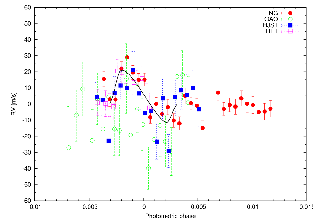
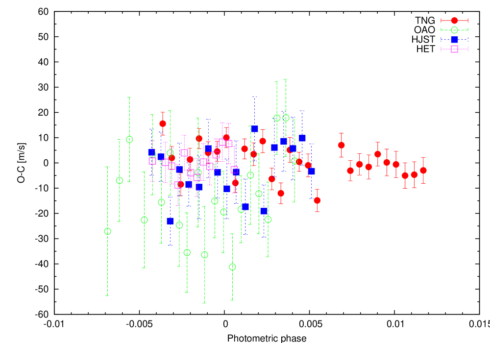
Figure 9: Upper panel: residuals of radial velocities of HD 17156 phased to the best-fit orbital solution with the best fitted Rossiter-Mclaughlin effect overlayed. Bottom panel: residuals from the Rossiter-Mclaughlin effect.

Table 5: Results of the Rossiter-McLaughlin modeling of all datasets. (OAO: Narita et al dataset).

telescope	date	v$\sin i$	$\lambda$	$\chi^{2}$
		$\rm km\,/s$	deg
OAO	17/11/2007	1.8 $\pm$ 1.5	-22.6 $\pm$ 20.3	0.7
TNG	3/12/2007	1.5 $\pm$ 0.7	4.8 $\pm$ 5.3	1.4
HJST	25/12/2007	2.2 $\pm$ 1.0	0.8 $\pm$ 6.4	0.9
HET	25/12/2007	1.0 $\pm$ 5.0	30.1 $\pm$ 25.6	0.3
TNG+HJST		1.6 $\pm$ 1.0	3.9 $\pm$ 5.4	1.2

We also measured line bisectors and bisector velocity span using the technique developed by Martínez Fiorenzano et al. (2005) and looked for changes in the line profiles caused by the planetary transit (see Loeillet et al. 2008). We do not detect significant variations (Fig. 10). This is not unexpected considering the typical signal to noise ratio of our spectra and the low amplitude of the Rossiter signature.

Figure 10: Bisector velocity span (BVS) from line bisectors of HD 17156 spectra. Upper panel displays BVS vs. RV. Lower panel shows the line bisectors from all spectra, where the horizontal lines enclose the top and bottom zones considered to compute the BVS.

6 Clues on additional companions

HD 17156 was observed with AdOpt@TNG, the adaptive optics module of TNG (Cecconi et al., 2006). The instrument feeds the HgCdTe Hawaii 1024x1024 detector of NICS, the near infrared camera and spectrograph of TNG, providing a field of view of about 44 $\times$ 44 arcsec, with a pixel scale of 0.0437 ″/pixel. Plate scale and absolute detector orientation were derived in a companion program of follow-up of binary systems with long term radial velocity trends from the SARG planet search (Desidera et al., 2007).

Series of 15 sec images on HD 17156 were acquired on 3, 18 and 23 October 2007 in Br$\gamma$ intermediate-band filter. Images were taken moving the target in different positions on the detector, to allow sky subtraction without the need for additional observations, and each night at three different field orientations to make it easier to disentangle true companions from image artifacts. The target itself was used as reference star for the adaptive optics. Observing conditions were poor on the night of October 3, and rather good on the nights of 18 and 23 October, when we obtained a typical Strehl Ratio of about 0.3.

Data reduction was performed by first correcting for detector cross-talk using dedicated routines and then performing standard image preprocessing (flat fielding, bad pixels and sky background corrections) in the IRAF environment. Individual images taken at a fixed orientation were shifted and coadded.

The successive analysis was optimized for the detection of companions in different separation ranges. At small separations (from about 0.15 to 2 arcsec) we selected the two best combined images taken at different field orientations on 2007 Oct 18. They are shown in Fig. 11. These two sets of images are characterized by similar patterns of optical aberrations, and therefore, considering their difference, most of the patterns cancel out in difference images (Fig. 11), improving significantly the detection limits (angular differential imaging, Marois et al. (2006)). In the differential image, a true companion is expected to show two peaks, one positive and one negative, at the same projected separation from the central star and position angle displaced by 20^∘ (the rotation angle between the two sets of images in our case). For detection at separations larger than about 2 arcsec, we summed all the images after an appropriate rotation, obtaining a deep image over a field of about 10$\times$10 arcsec.

No companion was seen in both the differential image at small separation and in the deep combined image within 10 arcsec. The limit for detection was fixed at peak intensities 5 times larger than the dispersion over annuli at different radial separation. The results, both for the differential image and the deep composite image are shown in Fig. 12.

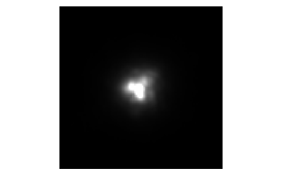
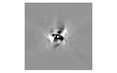
Figure 11: Images of HD 17156 . Upper panel: image of HD 17156 obtained with ADOPT@TNG. A similar quasi-static speckle pattern can be seen. Lower panel: difference between two images taken with two different field orientations, which allows to improve significantly detection limits in the inner regions. The field of view shown is 4.3x4.3″. The images are displayed in linear gray scale.

Figure 12: Detectability limits for companions of difference magnitude around HD 17156 as a function of the projected separation in arcsec Continuous line: limits on the difference image. Dotted line: limits on the composite deep image.

The contrast limits derived above were transformed into limits on companion masses using the mass-luminosity relation by Delfosse et al. (2000), and projected separation in arcsec to AU using the Hipparcos distance to the star (Fig. 13). A main-sequence companion can be excluded at a projected separation between about 150 and 1000 AU (the limit of image size). At such separations only brown-dwarf or white-dwarf companions are compatible with our detection limits. At smaller separation, detectability worsens quickly, and only stars with mass larger than about 0.4 M_⊙ can be excluded at projected separations closer than $\sim 50$ AU.

Figure 13: Detectability limits for stellar companions around HD 17156 as a function of the projected separation in AU. Continuous line: limits on the difference image dotted line: limits on the composite deep image.

The residuals from the radial velocity orbital solution do not suggest the occurrence of long term trends. This places further constraints on the binarity of the target. However, the timespan is rather short, and the continuation of the radial velocity monitoring is mandatory for a more complete view.

The available astrometric data from Hipparcos does not show evidence for stellar companions either (no astrometric acceleration within the timespan of the Hipparcos observations and no significant differences between

7 Summary and Discussion

In this paper, we studied the characteristics of HD 17156 and its transiting planets. Stellar parameters (mass, radius, metallicity) agree quite well with the previous study by F07.

Our measurement of the stellar radius of HD 17156 obtained through the analysis of the transit light-curve is the same as the one obtained using the Stefan-Boltzmann law or the Kervella calibration (Tab.2). Gillon et al. (2008) obtained a radius of 1.63 $\pm 0.2$ R_⊙, which is only marginally compatible with our estimate 1.44 $\pm 0.08$ R_⊙. On the one hand, to explain such a large stellar radius and the observed visual magnitude, it would be necessary to add $\sim 0.3$ mag of interstellar absorption, that at the distance of HD 17156 is not realistic (suggesting a mean extinction of 4 mag/kpc) because HD 17156 is located well inside of the Local Bubble, where no strong absorption is present, and the maximum expected absorption is few hundreds of mag. On the other hand, also the comparison of the Gillon et al. (2008) radius estimate with stellar models does not appear satisfactory: it is not possible to find model with a radius that agrees with the observed temperature and metallicity of HD 17156 . We conclude that the determination of the stellar radius, and by inference planetary radius, Gillon et al. (2008) is overestimated by 15%.

For a planet of 3M_J and an age of $\sim 2$ Gyr, theoretical models of planet evolution (Baraffe et al., 2008) predict a radius ranging between 0.9 and 1.1R_J as a function of chemical composition of the planet. Our determination of the radius of HD 17156b is $R_{p}=1.02\pm 0.08$ R_J. This is in excellent agreement theoretical expectations. Thus, the strong tidal heating effects on the planet do not appear to contribute to significantly inflate its radius.

Fortney et al. (2007) suggested that HD 17156b , due to its large orbital eccentricity, can change its spectral type during the orbit from a warm pL type at apoastron to a hotter pM type at periastron. Their models suggest that for pM class planets the observed radius at R band could be 5% larger than the radius measured at B band (due to the increased opacity of TiO and VO in the R band). Comparing our radius measurements in the R band and the measurements obtained in the B band by Gillon et al. (2008), we find identical results. This result is however not significant because of the large error involved in radius measurement. In order to obtain a significant difference of the radius in B and R band each measurement should be more accurate than 0.03 R_J.

Our RV monitoring of HD 17156 during the 2007 December 3 transit does not confirm the misalignment between the stellar spin and planet orbit axes claimed by Narita et al. (2008), but it agrees instead with the opposite finding by Cochran et al. (2008). We think our results are more robust because the other most accurate dataset (HET in Cochran et al. 2008) does not cover the full transit, leaving some uncertainties in their Rossiter modeling. We then conclude that the projection on the sky of the stellar spin and planet orbit axes are aligned to better than 10 deg.

Therefore HD 17156 joins most of the other exoplanet systems with available measurements of the Rossiter-McLaughlin effect in being compatible with coplanarity. The only possible exception is represented by the XO-3 system, for which Hébrard et al. (2008) found indications for a large departure from coplanarity ($\sim 70^{\circ}$). However, as acknowledged by the authors, this result should be taken as preliminary, because of the possibility of unrecognized systematic errors for observations taken at large airmass and with significant moonlight contamination.

Our result confirms that large deviations from coplanarity between stellar spin and planet orbit axes are at most rather rare. Such a rarity had already been established at a high confidence level for the “classical” Hot Jupiters in short-period circular orbits. For massive eccentric planets the situation is less clear: HD 147506b ($M=8.6$ M_J , $P=5.6$ days, $e=0.52$) and HD 17156 ($M=3.2$ M_J , $P=21$ days, $e=0.67$) have projected inclinations below 10^∘ while the possible detection of spin-orbit misalignment in the XO-3 system ($M=12.5$ M_J, $P=3.2$ days, $e=0.29$) still awaits confirmation as discussed above.

The results of the spin-orbit alignment measurements for the HD 17156 system can be compared with the prediction of the planet scattering models. A range of alignments can be the outcome of planet-planet scattering (Marzari & Weidenschilling, 2002). Therefore, our indication for coplanarity does not exclude planet-planet scattering in the HD 17156 system. A larger number of transiting planets with significant eccentricities have to be discovered and characterized to get more conclusive inferences.

We also searched for stellar companions using adaptive optics, to test the hypothesis of Kozai mechanism to explain the large eccentricity of HD 17156 b. We did not detect companions within 1 000 AU, and our detection limits allowed us to exclude main sequence companions with projected separations from about 150 to 1 000 AU. This result makes unlikely the occurrence of a companion inducing Kozai eccentricity oscillations on the planet, but this possibility can not be yet completely rule out (companions at small projected separation and faint white dwarfs and brown dwarfs companion still possible). Continuation of radial velocity and photometric monitoring will allow a more complete view on the existence of additional companions at small separations.