Charm and longitudinal structure functions with the KLN model

Abstract

We use the Kharzeev-Levin-Nardi (KLN) model of the low $x$ gluon distributions to fit recent HERA data on $F_{L}$ and $F^{c}_{2}\,(F^{b}_{2})$. Having checked that this model gives a good description of the data, we use it to predict $F_{L}$ and $F^{c}_{2}$ to be measured in a future electron-ion collider. The results are similar to those obtained with the de Florian-Sassot and Eskola-Paukkunen-Salgado nuclear gluon distributions. The conclusion of this exercise is that the KLN model, simple as it is, may still be used as an auxiliary tool to make estimates both for heavy ion and electron-ion collisions.

The small-$x$ regime of QCD has been intensely investigated in recent years (for recent reviews see, e.g. cgc ; gllm ). The main prediction is a transition from the linear regime described by the DGLAP dynamics to a non-linear regime where parton recombination becomes important in the parton cascade and the evolution is governed by a non-linear equation. At very small values of $x$ we expect to observe the saturation of the growth of the gluon densities in hadrons and nuclei. One of the main topics of hadron physics to be explored in the new accelerators, such as the LHC and possibly the future electron-ion collider is the existence of this new component of the hadron wave function, denoted Color Glass Condensate (CGC) cgc .

The search for signatures of the CGC has been subject of an active research (for recent reviews see, e.g. cgc ). Saturation models gllm ; GBW ; bgbk ; kowtea ; iim ; fs can successfully describe HERA data in the small $x$ and low $Q^{2}$ region. Moreover, some properties which appear naturally in the formalism of the color glass condensate have been observed experimentally. These include, for example, geometric scaling bl ; scaling ; iimc and the supression of high $p_{T}$ hadron yields at forward rapidities in $dAu$ collisions brahms ; jamal ; kkt ; dhj ; gkmn ; buw . However, it has been shown that both geometric scaling caola and high $p_{T}$ supression kahana ; vogt04 can be understood with other explanations, not based on saturation physics.

In view of these (and others) results we may conclude that there is some evidence for saturation at HERA and RHIC. However, more definite conclusions are not yet possible. In order to discriminate between these different models and test the CGC physics, it would be very important to consider an alternative search. To this purpose, the future electron-nucleus colliders offers a promising opportunity raju_ea1 ; raju_ea2 ; raju_ea4 ; raju_ea5 ; kgn .

The color glass condensate is important in itself as a new state of matter. However, apart from that, we need to know very well its properties since the CGC forms the initial state of the fluid created in nucleus-nucleus collisions. Any detailed simulation of a heavy ion collision needs a realistic Ansatz for the initial conditions. This would correspond to knowing accurately the unintegrated gluon distribution in the projectile and in the target. These distributions will presumably be known in the future, with the help of the results of deep inelastic scattering (DIS) off nuclei. Even before experiment, one can try to calculate the gluon density in the initial state of heavy ion collisions by numerically solving the classical Yang-Mills equations, as done in kras . This is however very time consuming. Meanwhile, in practical applications we need to use use models for these distributions. Since these models are used as input for heavy numerical calculations, they have to be simple.

One simple approach to saturation physics was developed by Kharzeev, Levin and Nardi (KLN) in a series of papers kln , where a simple model for the unintegrated gluon distribution was proposed. It was used in many phenomenological applications. In particular it was very successful when applied to hydrodynamical simulations hirano04 , hirano042 and adil05 . In hirano04 it was shown that hydrodynamical simulations with the KLN model initial conditions were able to the describe centrality, rapidity and energy dependence of charged hadron multiplicities very well. Moreover these simulations could reproduce the transverse momentum spectra of charged pions and also the centrality dependence of the nuclear modification factors.

In view of the success of the KLN model as an input for numerical simulations, we think that it would be interesting to confront it with recent DIS data and, if necessary, change it in order to get a better agreement with these data. Of course, the KLN will remain a phenomenological model to be replaced by something more fundamental in the future. However, in a refined and still simple version, it may be a very useful tool, capturing the essential physics of gluon saturation and parameterizing the presently available experimental information.

In this paper we apply the KLN model to deep inelastic scattering, the domain where parton distributions have to be tested. If it fails badly in reproducing DIS data, it must be discarded. Since the KLN model gives only an Ansatz for the gluon distribution but says nothing about quarks, it is difficult to use it to make predictions for the most well known DIS observables, such as the structure functions $F_{2}$. We must then look for quantities which are dominated by the gluon content of the proton. These are the charm (bottom) and longitudinal structure functions, $F_{2}^{c}\,(F_{2}^{b})$ and $F_{L}$ respectively.

Let us first discuss charm production and its contribution to the structure function. In the last years, both the H1 and ZEUS collaborations have measured the charm component $F_{2}^{c}$ of the structure function at small $x$ and have found it to be a large (approximately $25\%$) fraction of the total f2cdata . This is in sharp contrast to what is found at large $x$, where typically $F_{2}^{c}/F_{2}\,\approx{\cal{O}}(10^{-2})$. This behavior is directly related to the growth of the gluon distribution at small-$x$.

In order to estimate the charm contribution to the structure function we consider the formalism developed in grvc where the charm quark is treated as a heavy quark and its contribution is given by fixed-order perturbation theory. This involves the computation of the boson-gluon fusion process $\gamma^{*}g\rightarrow c\overline{c}$. A $c\overline{c}$ pair can be created by boson-gluon fusion when the squared invariant mass of the hadronic final state is $W^{2}\geq 4m_{c}^{2}$. Since $W^{2}=\frac{Q^{2}(1-x)}{x}+M_{N}^{2}$, where $M_{N}$ is the nucleon mass, the charm production can occur well below the $Q^{2}$ threshold, $Q^{2}\approx 4m_{c}^{2}$, at small $x$. The charm contribution to the proton/nucleus structure function, in leading order (LO), is given by grv95

$$\frac{1}{x}F_{2}^{c}(x,Q^{2},m_{c}^{2})=e_{c}^{2}\frac{\alpha_{s}(\mu^{2})}{2\pi}\int_{ax}^{1}\frac{dy}{y}\,C_{g,2}^{c}(\frac{x}{y},\xi)\,g(y,\mu^{2})\,\,,$$ (1)

where $a=1+\xi$ ($\xi\equiv\frac{m_{c}^{2}}{Q^{2}}$) and the renormalization scale $\mu$ is assumed to be either $\mu^{2}=4m_{c}^{2}$ or $\mu^{2}=4m_{c}^{2}+Q^{2}$. $C_{g,2}^{c}$ is the coefficient function given by

$$C_{g,2}^{c}(z,\xi)=\{[z^{2}+(1-z)^{2}+4\,\xi\,z\,(1-3z)-8\,\xi^{2}\,z^{2}]$$ (2)

$$\times ln\,H+\beta\,[-1+8\,z\,(1-z)-4\,\xi\,z\,(1-z)]\}\,\,,$$

where $\beta=1-\frac{4\,\xi\,z}{(1-z)}$ and $H=\frac{1+\beta}{1-\beta}$.

The dominant uncertainty in QCD calculations comes from the uncertainty in the charm quark mass. In this paper we assume $m_{c}=1.2\,$ GeV. In (1) $g(y,\mu^{2})$ is the gluon distribution, which is usually taken from the CTEQ cteq , MRST mrst or GRV grv98 parameterizations. In what follows we shall use the KLN Ansatz:

$$xg(x,Q^{2})=\left\{\begin{array}[]{ll}\frac{\kappa_{0}}{\alpha_{s}(Q_{s}^{2})}\,S\,Q^{2}\,(1-x)^{D}&,\,\,\,\textrm{$Q^{2}<Q_{s}^{2}$}\,\,,\\ \frac{\kappa_{0}}{\alpha_{s}(Q_{s}^{2})}\,S\,Q_{s}^{2}\,(1-x)^{D}&,\,\,\,\textrm{$Q^{2}>Q_{s}^{2}$}\,\,.\end{array}\right.$$ (5)

In the above expression $S$ is the area of the target and $\alpha_{s}$ is the running coupling $\alpha_{s}={12}/[25\pi\,ln(Q^{2}/\Lambda^{2})]$ (with $\Lambda=0.224$ GeV). In (5) $D=4$ and $\kappa_{0}$ is a constant parameter to be adjusted by requiring that the distribution $xg(x,Q^{2})$ satisfies the momentum sum rule $\int_{0}^{1}dx\,xg(x,Q^{2})=p$, where $p$ is the value obtained with the GRV98 gluon density. $Q_{s}$ is the saturation scale given by:

$$Q_{s}^{2}(x)=Q_{0}^{2}\left(\frac{x_{0}}{x}\right)^{\lambda}$$ (6)

where $Q_{0}^{2}=0.34~{}~{}GeV^{2}$, $x_{0}=3.0\times 10^{-3}$ and $\lambda=0.25$.

In Fig. 1 we show $F_{2}^{c}$ as a function of $x$ obtained with the above expression and compared to the ZEUS and H1 data. Solid and dashed lines correspond to different choices for the renormalization scale. We can observe that there is a surprisingly good agreement between the KLN model and the data, especially considering that only minor changes in the parameters were made, with respect to those found previously in the analysis of RHIC data kln . We can also obtain a reasonable description of large $Q^{2}$ data, which is also surprising because the KLN model has no DGLAP evolution, being tuned to the low $x$ and low $Q^{2}$ region of the phase space, where gluon saturation is expected to occur. In Fig. 2 we show the results for $F_{2}^{b}$ and compare them with the H1 data f2cbdata . With the exception of the points with $Q^{2}=200$ GeV², the agreement with data is similar to the one found for $F_{2}^{c}$.

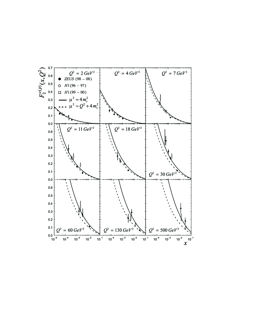
Figure 1: Charm structure function, $F_{2}^{c}$ computed with the KLN model. Data are from Ref. f2cdata .

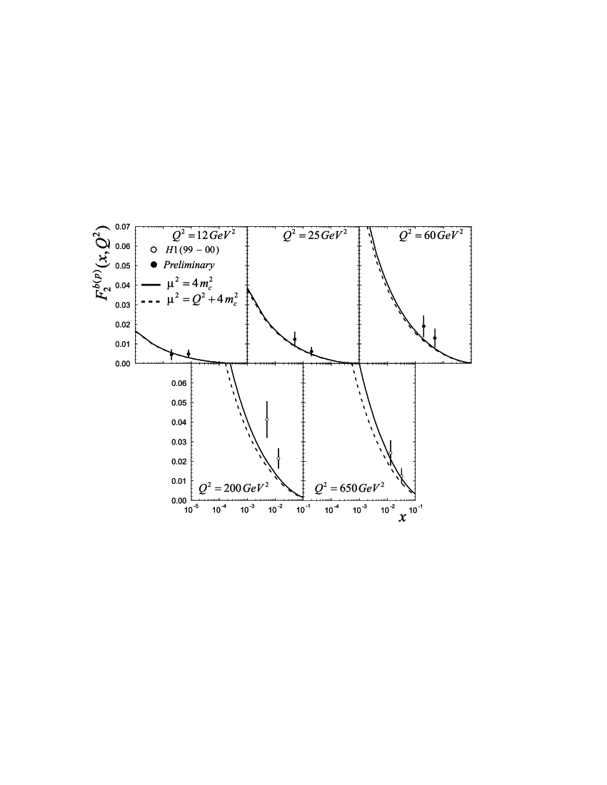
Figure 2: Bottom structure function, $F_{2}^{b}$ computed with the KLN model. Data are from Ref. f2cdata .

New experimental HERA data on $F_{L}$ have recently appeared fldata08 . The longitudinal structure function in deep inelastic scattering is one of the observables from which the gluon distribution can be unfolded. Longitudinal photons have zero helicity and can exist only virtually. In the quark model, helicity conservation of the electromagnetic vertex yields the Callan-Gross relation, $F_{L}=0$, for scattering on quarks with spin $1/2$ vicmagfl . This does not hold when the quarks acquire transverse momenta from QCD radiation.

Instead, QCD yields the Altarelli-Martinelli equation alta

$$F_{L}(x,Q^{2}) = \frac{\alpha_{s}(Q^{2})}{2\pi}\,x^{2}\int_{x}^{1}\frac{dy}{y^{3}}\,[\frac{8}{3}\,F_{2}(y,Q^{2})$$ (7)

$$+ 4\,\sum_{q}e_{q}^{2}\,(1-\frac{x}{y})\,y\,g(y,Q^{2})]\,\,,$$

expliciting the dependence of $F_{L}$ on the strong coupling constant and the gluon density. At small $x$ the second term with the gluon distribution is the dominant one. In Ref. cooper the authors have suggested that expression (7) can be reasonably approximated by $F_{L}(x,Q^{2})\approx 0.3\,\frac{4\alpha_{s}}{3\pi}xg(2.5x,Q^{2})$, which demonstrates the close relation between the longitudinal structure function and the gluon distribution.

In what follows we calculate $F_{L}$ using the Altarelli-Martinelli equation, neglecting the $F_{2}$ contribution and using (5) in (7). The results are presented in Fig. 3, where they are compared with the very recent H1 data fldata08 and with the results obtained with the help of other standard gluon distribution functions. The agreement between the KLN predictions and data is remarkably good. This is again surprising because the KLN distribution is not expected to work so well at such large values of $Q^{2}$. The good agreement indicates that the KLN distribution has a good asymptotic behavior and it is compatible both with the data and with the other standard gluon distributions.

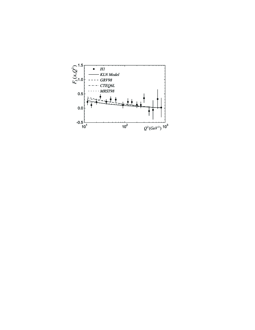
Figure 3: Longitudinal structure function $F_{L}$ computed with the KLN model and with the gluon distributions taken from CTEQ6L (dash dotted line), MRST98 (dotted line) and GRV98 (dashed line). Data are from Ref. fldata08

.

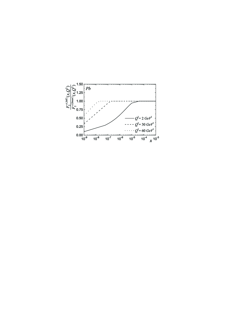
Figure 4: Ratio full to linear (explained in the text) $F^{cA}_{2}$ for $A=208$.

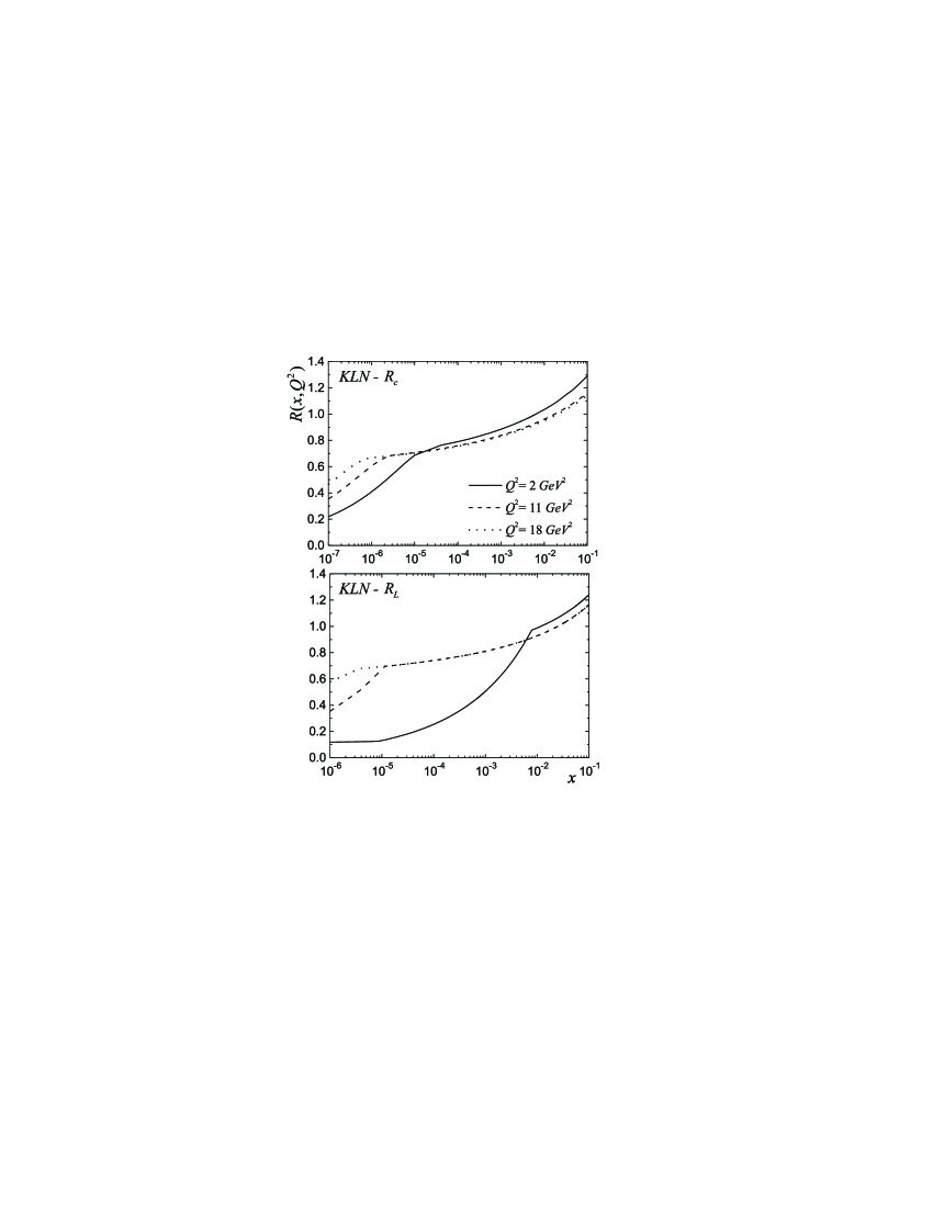
Figure 5: Ratios $R_{c}$ (top) and $R_{L}$ (bottom) predicted by the KLN model for $A=208$ and different values of $Q^{2}$.

Having checked that the KLN distribution reproduces satisfactorily the existing DIS data on electron-proton collisions, we shall now use it to make predictions for electron-ion collisions. The expression for the nuclear charm structure function $F^{c,A}_{2}$ is the same except for the change $g(y,Q^{2})\rightarrow g^{A}(y,Q^{2})$, where $g^{A}(y,Q^{2})$ is obtained from Eq. (5) with the replacements $S\rightarrow S^{A}=A^{2/3}S$ and $Q^{2}_{s}\rightarrow Q^{2A}_{s}$, where $Q^{2A}_{s}=A^{1/3}Q^{2}_{s}$. In order to estimate the strength of non-linear effects in $eA$ processes, we can compute the linear contribution to $F^{cA}_{2}$ using only the second line of Eq. (5). We call this $F_{2}^{c(linear)}$ and compare it with $F_{2}^{c(full)}$, where the latter is calculated with both lines of Eq. (5) and thus includes non-linear effects. The ratio $F_{2}^{c(full)}/F_{2}^{c(linear)}$ as a function of $x$ is shown in Fig. 4 for $A=208$ and for several values of $Q^{2}$.

The deviation of this ratio from unity shows the importance of non-linear effects. As expected, for large $x$ and for large $Q^{2}$ there are no saturation effects. In fact, saturation effects are only noticeable at $x<10^{-6}$ and for small values of $Q^{2}$. This result confirms the findings of erike1 , where an estimate of saturation effects in $eA$ collisions performed with the color dipole approach also led to the conclusion that they are only marginally visible in $F^{c,A}_{2}$. Having an idea of where saturation effects could be relevant, we can compute an observable quantity, which is $R_{c}(x,Q^{2})={F_{2}^{c,A}(x,Q^{2})}/{AF_{2}^{c,p}(x,Q^{2})}$. The deviation from unity in this ratio is an indication of saturation physics. A depletion in this ratio is called “shadowing”, whereas an enhancement is called “anti-shadowing”.

In Fig. 5 on the top panel we calculate $R_{c}$ and estimate the magnitude of shadowing, which can be of 50 % at very low (but still reachable) values of $x$ and $Q^{2}$. The equivalent ratio for the longitudinal structure functions $R_{L}(x,Q^{2})={F_{L}^{A}(x,Q^{2})}/{AF_{L}^{p}(x,Q^{2})}$ is shown in the bottom panel of Fig. 5 for the same choices of $Q^{2}$. We observe that significant non-linear effects start to appear at larger values of $x$. $R_{L}$ seems thus more promising than $R_{c}$. Following erike1 we compare the normalized ratios $R_{c}$ and $R_{L}$ obtained with the KNL model with the same ratios computed with the standard collinear factorization approach with nuclear parton distribution functions (nPDF’s). We take two extreme cases, one with almost no shadowing at all, based on the nPDF’s of de Florian and Sassot (called here DS) ds04 and one with maximum shadowing based on the Eskola, Paukkunen and Salgado nPDF’s (called here EPS) eps08 .

The ratios $R_{c}$ and $R_{L}$ are shown in Figs. 6 and 7 respectively. From the figures we see that the KLN model interpolates between the two extreme parameterizations, DS and EPS, being closer to the latter. This is expected, since the EPS gluon distribution comes from a fit of world data where BRAHMS data on forward particle production were included. Both KLN and EPS take RHIC data into account.

In summary, we have used the KLN model for the low $x$ gluon distributions, slightly changing the parameters fixed from previous analysis, to fit HERA data on $F_{L}$ and $F^{c}_{2}$. Having checked that this model gives a good description of the data, we have used it to predict $F_{L}$ and $F^{c}_{2}$ to be measured in electron-ion collisions. The results are close to those obtained with the DS and EPS nuclear gluon distributions. The conclusion of this exercise is that the KLN model, simple as it is, may still be used as an auxiliary tool to make estimates both for heavy ion and electron-ion collisions.

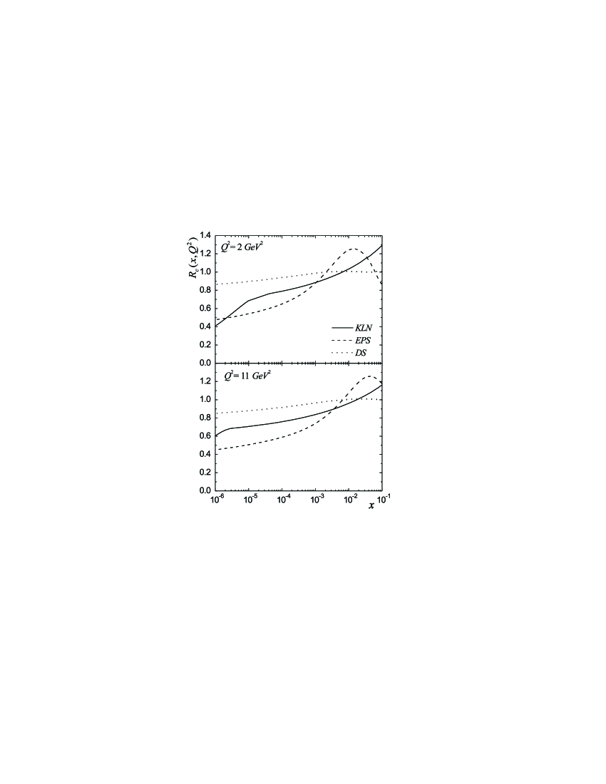
Figure 6: Ratio $R_{c}$ calculated with the KLN, DS and EPS nuclear gluon distribution functions for $A=208$ and $Q^{2}=2$ (top) and $Q^{2}=11$ (bottom) GeV².

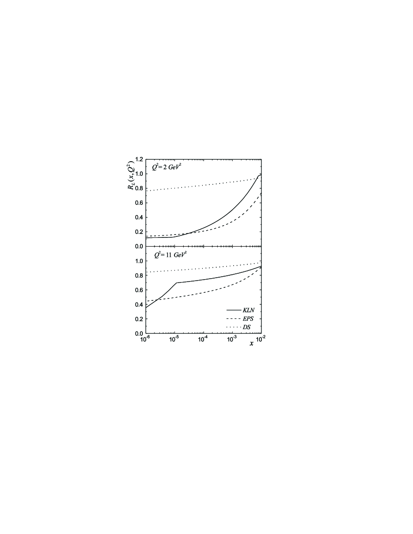
Figure 7: Ratio $R_{L}=$ calculated with the KLN, DS and EPS nuclear gluon distribution functions for $A=208$ and $Q^{2}=2$ (top) and $Q^{2}=11$ (bottom) GeV².

- (1) E. Iancu and R. Venugopalan, arXiv:hep-ph/0303204; A. M. Stasto, Acta Phys. Polon. B35, 3069 (2004); H. Weigert, Prog. Part. Nucl. Phys. 55, 461 (2005); J. Jalilian-Marian and Y. V. Kovchegov, Prog. Part. Nucl. Phys. 56, 104 (2006).
- (2) E. Gotsman, E. Levin, M. Lublinsky and U. Maor, Eur. Phys. J. C27, 411 (2003).
- (3) K. Golec-Biernat and M. Wüsthoff, Phys. Rev. D59, 014017 (1999), ibid. D60, 114023 (1999).
- (4) J. Bartels, K. Golec-Biernat, H. Kowalski, Phys. Rev. D66, 014001 (2002).
- (5) H. Kowalski and D. Teaney, Phys. Rev. D68, 114005 (2003).
- (6) E. Iancu, K. Itakura, S. Munier, Phys. Lett. B590, 199 (2004).
- (7) J. R. Forshaw and G. Shaw, JHEP 0412, 052 (2004).
- (8) J. Bartels and E. Levin, Nucl. Phys. B387, 617 (1992).
- (9) A. M. Staśto, K. Golec-Biernat and J. Kwieciński, Phys. Rev. Lett. 86, 596 (2001); V. P. Gonçalves and M. V. T. Machado, Phys. Rev. Lett. 91, 202002 (2003); N. Armesto, C. A. Salgado and U. A. Wiedemann, Phys. Rev. Lett. 94, 022002 (2005); C. Marquet and L. Schoeffel, Phys. Lett. B639, 471 (2006).
- (10) E. Iancu, K. Itakura and L. McLerran, Nucl. Phys. A708, 327 (2002).
- (11) I. Arsene et al. [BRAHMS Collaboration], Phys. Rev. Lett. 91, 072305 (2003); Phys. Rev. Lett. 93, 242303 (2004); Phys. Rev. Lett. 94, 032301 (2005).
- (12) J. Jalilian-Marian, Nucl. Phys. A748, 664 (2005).
- (13) A. Dumitru, A. Hayashigaki and J. Jalilian-Marian, Nucl. Phys. A765, 464 (2006); Nucl. Phys. A770, 57 (2006).
- (14) D. Kharzeev, Y.V. Kovchegov and K. Tuchin, Phys. Lett. B599, 23 (2004).
- (15) V. P. Goncalves, M. S. Kugeratski, M. V. T. Machado and F. S. Navarra, Phys. Lett. B643, 273 (2006).
- (16) D. Boer, A. Utermann and E. Wessels, Phys. Rev. D77, 054014 (2008).
- (17) F. Caola and S. Forte, Phys. Rev. Lett. 101, 022001 (2008).
- (18) D. E. Kahana and S. H. Kahana, J. Phys. G35, 025102 (2008).
- (19) R. Vogt, Phys. Rev. C70, 064902 (2004).
- (20) R. Venugopalan, AIP Conf. Proc. 588, 121 (2001); arXiv:hep-ph/0102087.
- (21) A. Deshpande, R. Milner, R. Venugopalan and W. Vogelsang, Ann. Rev. Nucl. Part. Sci. 55, 165 (2005).
- (22) H. Kowalski, T. Lappi and R. Venugopalan, Phys. Rev. Lett. 100, 022303 (2008) .
- (23) H. Kowalski, T. Lappi, C. Marquet and R. Venugopalan, arXiv:hep-ph/0805.4071.
- (24) M. S. Kugeratski, V. P. Goncalves and F. S. Navarra, Eur. Phys. J. C46, 413 (2006); Eur. Phys. J. C46, 465 (2006).
- (25) A. Krasnitz, Y. Nara and R. Venugopalan, Nucl. Phys. A727, 427 (2003).
- (26) D. Kharzeev, E. Levin and M. Nardi, Phys. Rev. C71, (2001), 054903; Nucl. Phys. A730, 448 (2004). Erratum-ibid. A743, 329 (2004); Nucl. Phys. A747, 609 (2005).
- (27) T. Hirano and Y. Nara, Nucl. Phys. A743, 305 (2004).
- (28) T. Hirano and Y. Nara, J. Phys. G31, S1 (2005).
- (29) A. Adil, M. Gyulassy and T. Hirano, Phys. Rev. D73, 074006 (2006).
- (30) C. Adloff et al. [H1 Collaboration], Z. Phys. C72, 593 (1996); J. Breitweg et al. [ZEUS Collaboration], Phys. Lett. B407, 402 (1997); C. Adloff et al. [H1 Collaboration], Phys. Lett. B528, 199 (2002); S. Aid et. al., [H1 Collaboration], Z. Phys. C72, 539 (1996); J. Breitweg et. al., [ZEUS Collaboration], Eur. Phys. J. C12, 35 (2000); S. Chekanov et. al., [ZEUS Collaboration], Phys. Rev. D69, 012004 (2004).
- (31) M. Gluck, E. Reya and M. Stratmann, Nucl. Phys. B422, 37 (1994).
- (32) M. Gluck, E. Reya and A. Vogt, Z. Phys. C67, 433 (1995).
- (33) H. L. Lai et al. [CTEQ Collaboration], Eur. Phys. J. C12, 375 (2000).
- (34) A. D. Martin, R. G. Roberts, W. J. Stirling and R. S. Thorne, Eur. Phys. J. C35, 325 (2004).
- (35) M. Gluck, E. Reya and A. Vogt, Eur. Phys. J. C5, 461 (1998).
- (36) A. Aktas et. al., [H1 Collaboration], Eur. Phys. J. C40, 349 (2005); A. Aktas et. al., [H1 Collaboration], Eur. Phys. J. C45, 23 (2006).
- (37) F.D. Aaron et. al, Phys. Lett. B665, 139 (2008); V. Chekelian, arXiv:hep-ex/0810.5112; M. Klein, arXiv:hep-ex/0810.3857.
- (38) For a recent discussion of the subject see: V. P. Goncalves and M. V. T. Machado, Eur. Phys. J. C37, 299 (2004); M. V. T. Machado, Eur. Phys. J. C47, 365 (2006).
- (39) G. Altarelli and G. Martinelli, Phys. Lett. B76, 89 (1978).
- (40) A. M. Cooper-Sarkar et al., Z. Phys. C39, 281 (1988).
- (41) E. R. Cazaroto, F. Carvalho, V. P. Goncalves and F. S. Navarra, Phys. Lett. B671, 233 (2009).
- (42) D. de Florian and R. Sassot, Phys. Rev. D69, 074028 (2004).
- (43) K. J. Eskola, H. Paukkunen and C. A. Salgado, JHEP 0807, 102 (2008).